Using Machine Learning on Macroeconomic, Technical, and Sentiment Indicators for Stock Market Forecasting

Abstract

Financial forecasting is a research and practical challenge, providing meaningful economic and strategic insights. While Machine Learning (ML) models are employed in various studies to examine the impact of technical and sentiment factors on financial markets forecasting, in this work, macroeconomic indicators are also combined to forecast the Standard & Poor’s (S&P) 500 index. Initially, contextual data are scored using TextBlob and pre-trained DistilBERT-base-uncased models, and then a combined dataset is formed. Followed by preprocessing, feature engineering and selection techniques, three corresponding datasets are generated and their impact on future prices is examined, by employing ML models, such as Linear Regression (LR), Random Forest (RF), Gradient Boosting (GB), XGBoost, and Multi-Layer Perceptron (MLP). LR and MLP show robust results with high R² scores, close to 0.998, and low error MSE and MAE rates, averaging at 350 and 13 points, respectively, across both training and test datasets, with technical indicators contributing the most to the prediction. While other models also perform very well under different dataset combinations, overfitting challenges are evident in the results, even after additional hyperparameter tuning. Potential limitations are highlighted, motivating further exploration and adaptation techniques in financial modeling that enhance predictive capabilities.

1. Introduction

Financial forecasting of stock markets has always been an objective of great interest in modern economies, where precision and timeliness can yield significant economic and strategic advantages. Accurate predictions of stock market movements have a great effect on investors, policymakers, and financial institutions’ decisions, which are important for resource allocation, risk management, and return maximization. In this remarkably demanding and dynamic environment of financial markets, changes in stock prices depend heavily on traditional financial indicators, but also on macroeconomic conditions and market sentiment that constantly change. Technological improvements have also increased access to data, giving the opportunity to exploit the computing power of advanced Machine Learning (ML) techniques, which capture complex patterns in financial time series, beyond traditional forecasting models [1].

Recent developments in financial market forecasting increasingly emphasize the effectiveness of Deep Learning (DL) models and the integration of sentiment analysis with traditional quantitative data. As highlighted in [2], financial markets are complex systems affected by a wide range of factors. Recent research demonstrates that combining sentiment information from sources, such as tweets analyzed using advanced Natural Language Processing (NLP) models like enhanced RoBERTa, with quantitative market data can notably improve predictive accuracy. LSTM models excelled in this integrated approach for forecasting the Tehran Stock Exchange. Moreover, the research in [3] systematically compares LSTM and GRU architectures for stock price prediction under identical conditions and finds that, while both models benefit from the inclusion of financial news sentiment, the presence of this sentiment data significantly enhances the performance of each, confirming its critical role in stock forecasting. Reinforcing these findings, the study in [4] shows that deep neural networks (DNNs) substantially outperform traditional models like Ordinary Least Squares (OLS) and historical averages in equity premium prediction, especially when enriched with a diverse set of financial variables.

Financial forecasting was used mainly to rely on either fundamental analysis or technical indicators to forecast stock prices, until great progress was made in advanced forecasting technologies. Fundamental analysis is a technique that focuses on analyzing the financial health of a company and market conditions, while Technical Analysis (TA) examines past price and volume information to identify trends and patterns.

While technology improvements have introduced the integration of more sophisticated models, including those based on ML algorithms, which exploit temporal dependencies in stock data to improve performance, most of the previous studies examined datasets that either combine technical and sentimental factors or used them in isolation, without considering the impact of macroeconomic elements [5,6,7,8,9,10,11,12].

Macroeconomic indicators are essentially the result of the economic conditions that shape future expectations, and their public announcement can act as a driver of market trends. While sentiment analysis has a great importance in market forecasting, it can partially reflect market behavior that guides future market fluctuations. Conversely, ML models provide the possibility to incorporate various features that capture complex, non-linear patterns in stock market forecasting, but prior studies tend to overlook fundamental economic elements when investigating these trends using ML models.

This study addresses this research gap by incorporating macroeconomic indicators with technical and sentiment-based features in the task of stock price predictions. Such a combination serves to enrich the feature space with varied inputs, further enabling the understanding of various market dynamics, which improves accuracy.

It mainly aims to predict the daily adjusted closing price of the US stock market, using an enriched feature dataset, and to find the most effective ML model for stock market prediction. Specifically, it combines indicators into one framework for unified forecasting.

Research Questions and Objectives

Although sentiment analysis and technical indicators have been widely used in financial forecasting, macroeconomic indicators, reflecting the broader economic sentiment, have been relatively unexplored in this domain [10,11,12]. The research questions addressed are:

• How do macroeconomic indicators impact stock market prediction when combined with technical and sentiment indicators?
• How well do different ML models capture and explain the impact of macroeconomic, technical, and sentiment indicators on stock prices?

To accomplish the above-mentioned aim, the following objectives are defined for the study:

• To create a sophisticated dataset leveraging macroeconomic, technical, and sentiment scoring indicators that will be utilized in the prediction of the daily adjusted closing price of the S&P 500 index. While the explainability of technical and sentiment indicators has been already studied in the literature, macroeconomic indicators signal different aspects of the economic state that can enhance the predictability of the stock index when they are combined with these indicators.
• To evaluate the efficiency of traditional and more advanced ML models, such as Linear Regression (LR), Random Forest (RF), Gradient Boosting (GB), XGBoost Regressor, and Multi-Layer Perceptron (MLP) in predicting stock prices. Each of these models leverage strengths of linear, tree-based, boosting, and related to Neural Network (NN) methods, such as the MLP model that can effectively capture the different aspects of the features and ensure a comprehensive stock index prediction.
• To identify the optimal combination of features, by applying feature selection techniques.
• To assess the contribution of each feature in the price movement by examining the performance through feature importance approach.

These objectives aim to enhance the state-of-the-art by investigating the integrated impact of macroeconomic conditions, technical indicators, and market sentiment on stock price predictions, and examines how ML models would perform under different feature combinations, with and without prior feature selection.

To accomplish the above objectives, this study utilized various techniques for sentiment scoring, data pre-processing and engineering, as well as feature selection, which generated a comprehensive dataset suitable to be utilized by the models. The models are trained, and their performance is evaluated, using Mean Absolute Error (MAE), Mean Squared Error (MSE) and R-squared (R²) which are more appropriate for continuous numerical predictions, since the study involves a regression task.

Overall, the study’s novelty lies in highlighting that a broader set of features enhances the predictability of ML models. However, limitations and weaknesses are also evident, based on the architecture developed, in terms of engineering and modeling, indicating the potential for improvement.

2. Background

In this section, the academic literature is outlined, spanning from the early approaches to predicting the stock market, up to the most advanced techniques implemented so far. In particular, the core theories and the TA fundamental approach are discussed, followed by the impact of sentiment analysis and the implementation from traditional to more advanced ML models.

Prior to any of the revolutionary studies that set the ground for the prevailing ML approaches for stock market prediction, the main prediction methods relied on fundamental analysis, TA, and market timing strategies. They were considered adequate to provide efficient estimations for future price movements. The ground for fundamental analysis was set by the study in [13] where the Efficient Market Hypothesis (EMH) and the Random Walk Theory (RWT) in stock prices were introduced. This means that stock prices incorporate any new available information and any changes that occur in price movements do not depend on past prices, and therefore they cannot affect future prices. An extensive overview of the EMH was later developed, suggesting that financial markets are efficient enough in reflecting all the available information in asset prices so that investors are unable to obtain abnormal returns on active trading and hence, modern passive investment strategies are possible to be applied [14].

The idea of predicting stock prices by applying TA and market timing strategies was initially established in Dow’s theory and is actively used in several different forms today [15]. As explained in [16], this theory suggests that stock market movements can be predicted based on patterns of historical price trends and trading volumes, since they carry all the investors psychology at the time of a historical event. Their consistent repetition on prices charts also provides confirmation for investors and professionals on the proactive decisions that they need to make.

This theory is also supported in [15] where it is implied that investors are confident to predict future price movements when patterns provided by TA methods are understood. This confidence is based on the foundation that all relevant information regarding a stock is fully captured in the price and volume movements. Therefore, analyzing historical patterns, investors shape anticipation for the next movements. In contrast to these beliefs though, the capability of price patterns to predict future movements has also been challenged. In [17], the ground for the effect of market efficiency in stock market price changes was established, suggesting that the behavior of stock price movement is random and therefore it does not depend on patterns.

2.1. Related Work

The following subsections present related studies examining the social emotion that drive market trends, followed by applications of traditional as well as advanced ML models on broader sets of features.

2.1.1. Sentiment Analysis in Stock Market Forecasting

The examination of sentiment information that stems from social media and its effect on stock price prediction has been studied extensively in the literature by incorporating data feeds mainly from Twitter (now X). In [18], public X posts and historical closing stock prices were analyzed using NLP and Data Mining (DM) techniques, suggesting the possibility of internal association in the multilayer hierarchical structures with 76.12% accuracy.

In [19], Support Vector Machines (SVM), Naïve Bayes Classifiers (NBC), Decision Trees (DT), RF and NN were employed to examine the effect of Twitter sentiment on the Indonesian stock market movement. With an accuracy of 60.39% and 56.5% RF and NBC, respectively, dominated other algorithms, while LR achieved a 67.73% accuracy on price prediction. The importance of Twitter (now X) data in the prediction of six banking stocks is also evident in [20], where a comparative analysis was conducted using k-Nearest Neighbors (KNN), Genetic Algorithms (GA), and Support Vector Regression (SVR) with and without assessing the sentiment effect.

In addition, the study in [21] analyzed financial news feeds related to Apple Inc. in a dictionary-based approach to positive and negative financial specific words. After employing models for classification and testing, it was found that RF provided the highest accuracy ranging from 88% to 92% followed by a significantly high accuracy rate of 86% by SVM, and 83% by NBC. Attaching sentiment analysis to the dataset was found to potentially increase the choice of a less riskier investment decision as model accuracy increased almost 75% compared to initial results where sentiment analysis was not applied to the data.

Focusing on the issue of noise inherent in social media datasets, the study in [11] employs PageRank in X posts to assess user importance and hence, prioritize relevant information by weighing X posts. Based on the input features, three different datasets were generated, called economic, sentiment, and PageRank-weighted sentiment, and five ML models were employed against the price of a 30-stock comprised portfolio. XGBoost was found to deliver the lowest errors for 13 stocks, with the greatest robustness across datasets, while the economic dataset was the only profitable among the datasets with a 0.75% cumulative return.

Moreover, the research in [22] proposes an innovative two-stage framework that integrates social media sentiment, processed through an Off-Policy Proximal Policy Optimization (PPO) algorithm. This addresses class imbalance, with historical stock data using a Transductive LSTM (TLSTM) to better capture temporal patterns, significantly outperforming both traditional and state-of-the-art DL models on Indian equities. Similarly, research in [23] demonstrates that sentiment indices extracted from European put and call option prices, incorporating both entropic and non-entropic measures of market pessimism, consensus, and optimism, offer substantial predictive power over longer horizons for both the S&P 500 and Bitcoin markets, especially under systemic shocks. Sentiment-driven models consistently outperformed benchmarks. Additionally, research in [24] further supports the synergy of news sentiment and numerical data, by introducing a hybrid FinBERT-LSTM model, which integrates sentiment analysis of financial news (via FinBERT) with technical time-series data. This yields superior accuracy on NASDAQ-100 stocks compared to LSTM and DNN baselines and emphasizes the value of weighted news categories and tailored NLP approaches.

An attempt to investigate the impact of public sentiment, derived mainly from Twitter (now X) and StockTwits, for the prediction of Microsoft stock price variations was reported in [10] by using KNN, SVM, LR, NBC, DT, RF, and Multilayer Perceptron (MLP). For the classification of consensus sentiment and its intensity, TextBlob and VADER sentiment analyzers employed in the X posts and results showed that the Twitter (now X) dataset produced reliable predictions for 15 continuous days of increases in stock prices using the SVM model, resulting in an F-score of 76.3% and an Area Under Curve (AUC) of 67%, especially when combined with VADER.

Other studies have also examined the effect of sentiment in stock market prediction by analyzing directly unstructured text data in the form of articles available from various sources, such as websites, mobile channels, or social networks [25]. In various studies, NBC was employed for document classification to categorize news polarities and perform sentiment analysis [26,27]. Meaningful stock prediction results with high accuracy were produced when datasets were enriched with more variables that reflect the stock price volatility.

Analyzing expressive attributes, such as market feedback, drastically improved the accuracy of the model employed, while a feedback-based feature selection with a combination of two words resulted in an even better accuracy of 76% [28]. In other text classification approaches, where categorization of article data was based on the level of word pairs [29], 61% accuracy was achieved when SVM was employed, while analyzing articles in categories, such as sub-industry and actual stock relevance, resulted in increased accuracy of 79.59% when polynomial kernels were applied [30].

Other NLP techniques such as tokenization, stemming, and stop word removal to extract relevant information in financial news articles were also performed in [31] so that their effect on stock price movement to be studied using an Improved Apriori Algorithm (IAA). The results of the study showed that IAA outperformed Apriori and Frequent Pattern (FP) growth in terms of accuracy and efficiency.

In a similar manner in [32], enhanced NLP techniques using a rule-based technique called the Mamdani Fuzzy Inference System (FIS) were employed to analyze the news articles and predict the stock market prices [32]. The results of the study showed that the Mamdani FIS model outperformed the other models in terms of predicting stock market prices using financial news articles.

Lastly, in contrast to previous studies, an attempt to analyze the effect of news headlines and descriptions on Microsoft, Tesla, and Apple stock prices was made in [33]. TextBlob was utilized to categorize sentiment, and the effectiveness of non-linear and linear models was examined. Results indicated that non-linear models, such as cubic regressions, encompass more predictive power for capturing stock price fluctuations.

2.1.2. Stock Market Forecasting Through Machine Learning

Other approaches to predict stock market movements using ML incorporated solely financial data. The study in [34] used DM techniques to examine the Kuwait stock market by applying LR, SVM, DT, and RF on historical stock prices and other fundamental financial indicators, such as oil price, gold price, the exchange rate of the Kuwaiti Dinar (KWD) to the US Dollar (USD), money supply, interest rate, Earnings Per Share (EPS), Dividends Per Share (DPS), and the Gulf stock market. The accuracy of the multinomial logic regression test was up to 54.24% while the confusion matrix of the polynomial kernel function of SVM achieved an accuracy of 52.73%, which was relatively lower. DT and RF test algorithms estimated accuracy almost at 53%. DT were also employed in [35], suggesting an effective tool for predicting the future prices of stocks.

In addition, an Evaluated Linear Regression-based ML (ELR-ML) technique on S&P 500 price index related data in [8] achieved moderate accuracy with a correlation (R²) of 0.358 and relatively accepted volatility prediction, considering that the dataset was spanning during the financial crisis period. Other studies have also employed traditional [5,36] and hybrid SVMs, such linear SVM [37] and GARCH-SVM [38] providing effective results. Other studies, such as [39], combine ML with SHAP technique to analyze feature importance in gold price movements. The best performance was found for XGBoost, yielding an R² of 0.994 and an RMSE of 34.921 which outperformed other models like CatBoost and RF, hence giving more confidence in its strong predictive ability.

NNs-related algorithms are also employed to a great extent in the literature, providing significant implications. In [40], the relationship between the S&P 500 stock market index and fundamental, macroeconomic, and technical data is investigated by applying single layer and multilayer LSTM architectures. For each architecture, different sets of hyperparameters were tested with the overall conclusion being that the single LSTM model with 150 hidden neurons provided the best fit and the highest prediction accuracy.

In another study, an optimal LSTM DL architecture and adaptive Stock Technical Indicators (STIs) concept are proposed to predict the price and trend of three banking stocks listed in National Stock Exchange (NSE) in India. The results of the optimal LTSM model are compared to SVM, LR, and one DL model (ELSTM) and show that the highest accuracy and mean accuracy are 65.64% and 59.25%, respectively, which are much higher than that of SVM, LR, and the DL approach (ELSTM) [6].

A complex NN architecture is also employed in [7] where LSTM and Gated Recurrent Unit (GRU) models are utilized for the prediction of economic trends and stock market prices. LSTM is built on an input layer that consists of a time series data over a defined previous period and an LSTM layer of 128 units, while the GRU model is built on a GRU layer with 128 units and two dense layers of 64 and 32 units, respectively, that lead to the final output layer. Results indicated that the LTSM model generally outperformed the GRU model, for most metrics, with a notably RMSE of 9.15 and MAE of 7.81 for Apple stock examination. Similarly, it outperformed other models like XGBoost ARIMA and Facebook Prophet algorithm, which were lagging significantly. Facebook Prophet algorithm is an open-source time series data prediction tool developed by Facebook that uses the additive regression model in the forecasting process.

Likewise, a DLWR-LSTM model construction is conducted to study short-term trends in China’s stock market in [41]. DLWR methodology is used to separate the stock data into distinct layers that represent strong trends, weak trends, and noise and then a model with three LSTM layers, two dense layers, and dropout is built to prevent overfitting. Prediction results indicated that the model effectively captured short-term trends as the number of separations increased and compared to other traditional approaches such as ARIMA, DLWR-ARIMA, and LSTM; the DLWR3-LSTM model provided the lowest MAPE and RMSE and R² close to 1, offering high accuracy and robustness across different market volatilities.

After combining technical indicators, financial ratios, and sentiment analysis, the study in [42] analyzed mid-term to long-term Taiwanese stock market trends by employing various ML models, such as RF, Feedforward NN, Gated Recurrent Unit and Financial Graph Attention Network (FinGAT). FinGAT provides the best results among other models regarding the High Portfolio Scores metrics, while for Excess Returns, both RF and FinGAT exceeded returns above 100% for all tested portfolios.

The efficiency of NNs versus traditional models, such as Ordinary Least Squares Regression (OLSR), is also studied in [43] where 21 independent variables related to macroeconomic conditions, market sentiment, and institutional factors are evaluated in order to predict the Shanghai Stock Exchange market volatility. Results indicate mixed implications, as NNs present higher capability in capturing complex patterns in the consumer goods and finance sectors, while traditional Ordinary Least Squares Regression method demonstrates higher accuracy in conglomerates, healthcare, and industrial goods sectors. A reinforcement learning Deep Double Q-Network (DDQN) algorithm is further developed in [9] for the prediction of NVIDIA. Applied in a three-phase approach, by progressively incorporating financial (phase 2) and sentiment indicators (phase 3) to the initial training phase of using only closing prices, results in an improved performance as far as the data complexity increases.

3. Data and Methods

This section details the methodological approach in this research, presenting each step of the process and analyzing the data utilized thoroughly.

Data creation and preprocessing are important steps for financial forecasting. An efficient database requires all relevant features, including technical indicators, macroeconomic data, and sentiment scores, to be collected and placed in some form of analytical format.

The financial dataset of this research was built on S&P 500 daily data, calculating technical indicators, while sentiment score was derived from news headlines. Macroeconomic indicators were retrieved directly from open access web sources, available in daily and monthly frequency.

Most of the preprocessing steps included resampling, filling monthly indicators with a forward fill approach, and applying lagged values with respect to capturing temporal dependencies. During preprocessing, the quality of the data was further enhanced by standardizing the formats, dealing with missing values, and matching data frequencies to ensure a consistent and accurate dataset on which models can efficiently be trained.

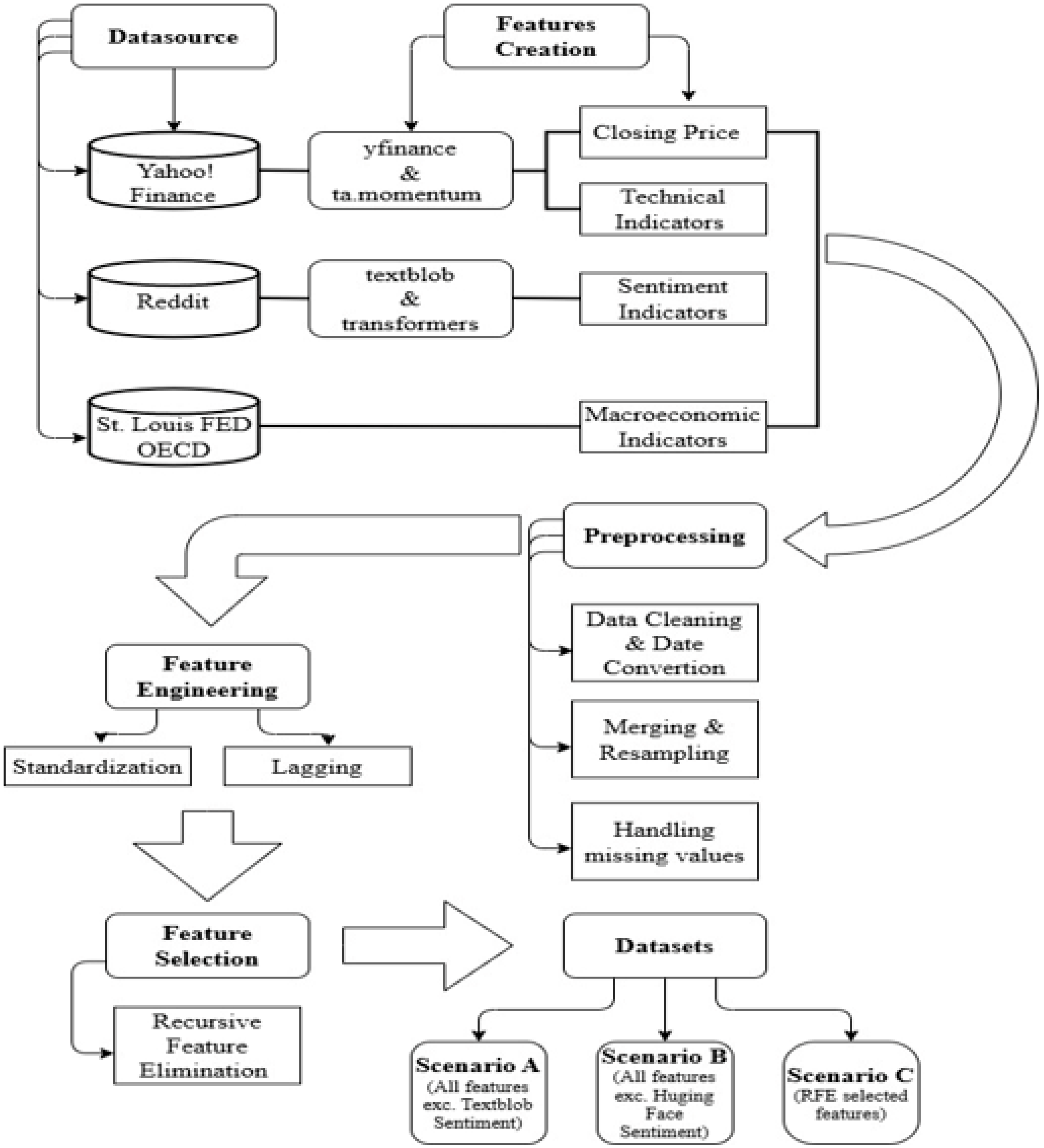
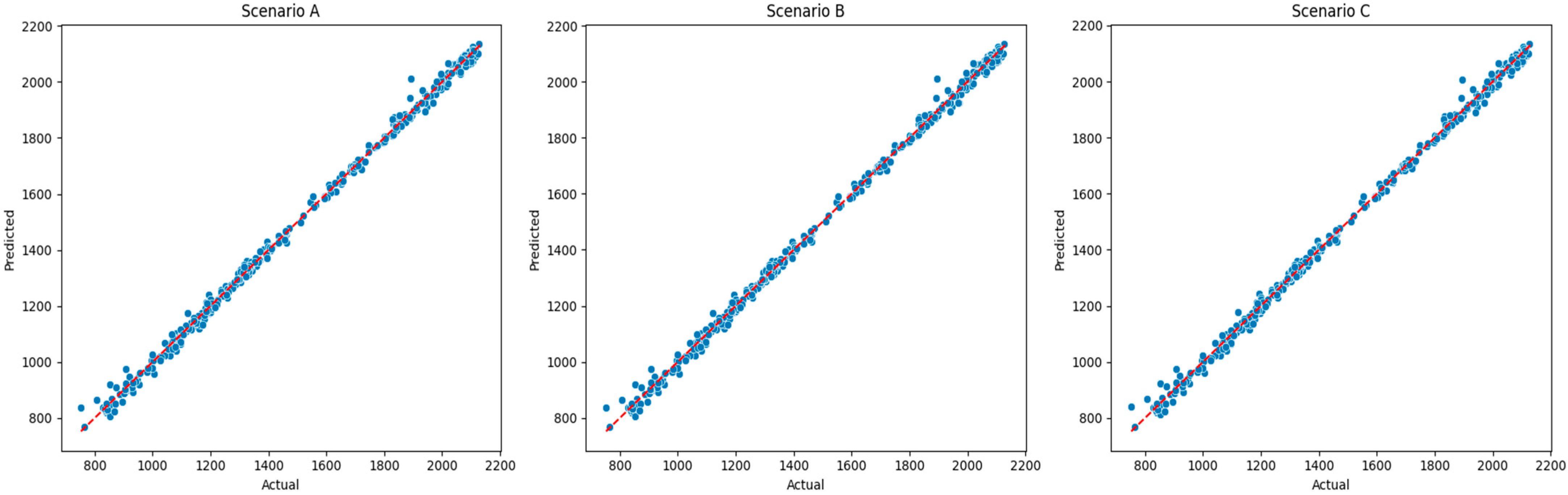
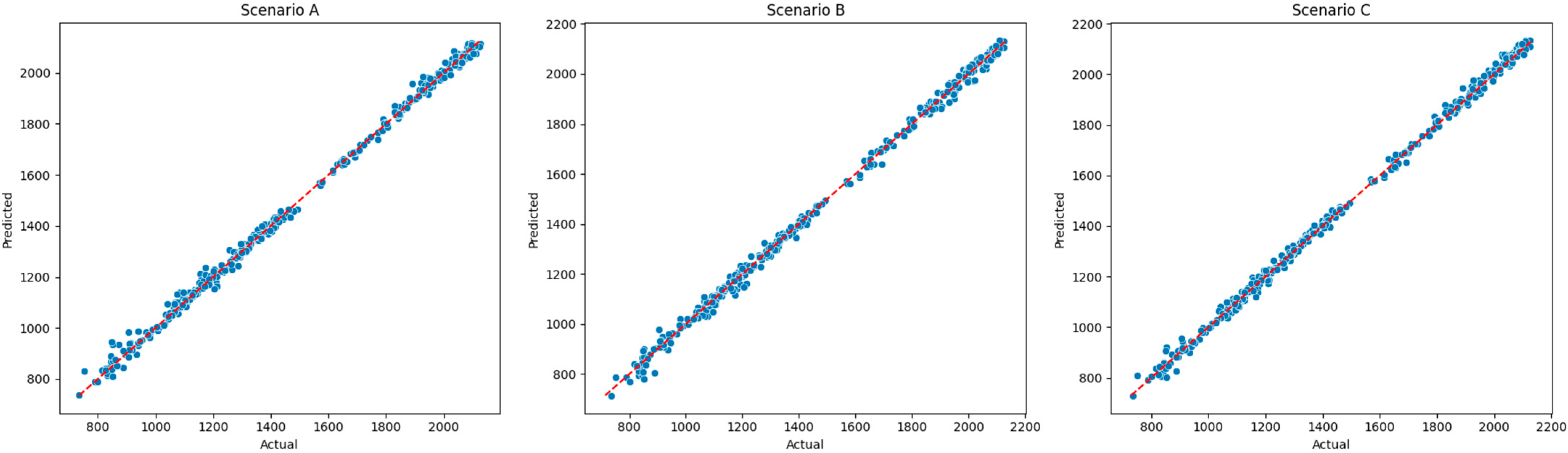
Feature engineering methods were also applied to ensure lower computational complexity. Based on the features created, two database scenarios (A and B) are initially generated differing only in the sentiment feature, in terms of the method employed for sentiment scoring. In addition, a feature selection technique is also employed to create Scenario C, based on the most important features. A sample of the final set of features, the standardized and lagged tested features and the actual values of the dependent variable against predicted values per scenario can be found in

Table A10. Sample dataset of engineered features after lag creation and target variable for the period 13–31 October 2014.

Date	Adj. Close	RSI	Stochastic Oscillator (%K)	Stochastic Oscillator (%D)	William (%R)	EMA	MACD Line	MACD Signal	MACD Diff	EPUI	EMUI	TB Yield 10Y	BCI	CEI	ISM PMI	Sentiment Score Textblob	Sentiment Score Pre-Trained DistilBERT
13/10	1874.74	45.58	1.18	25.88	−99.91	1955.79	−14.16	−7.28	−6.88	49.06	113.77	2.31	100.52	84.6	56.6	−0.04	−0.65
14/10	1877.7	43.01	0.41	7.35	−99.52	1944.98	−19.31	−9.69	−9.62	42.04	24.56	2.26	100.52	84.6	56.6	0.01	−0.75
15/10	1862.49	43.32	4.01	1.87	−95.29	1936.01	−22.89	−12.33	−10.57	62.32	9.09	2.21	100.52	84.6	56.6	0.03	−0.46
16/10	1862.76	42.12	21.06	8.49	−74.76	1926.21	−26.65	−15.19	−11.46	68.64	14.47	2.15	100.52	84.6	56.6	−0.04	−0.62
17/10	1886.76	42.15	21.20	15.42	−74.41	1917.75	−29.27	−18.01	−11.26	86.24	45.37	2.17	100.52	84.6	56.6	0.06	−0.26
20/10	1904.01	44.65	33.28	25.18	−59.82	1913.62	−29.08	−20.22	−8.85	49.35	83.92	2.22	100.52	84.6	56.6	0.03	−0.55
21/10	1941.28	46.36	41.97	32.15	−46.97	1912.34	−27.22	−21.62	−5.59	45.57	11.96	2.20	100.52	84.6	56.6	0.00	−0.59
22/10	1927.11	49.76	60.74	45.33	−23.26	1916.19	−22.47	−21.79	−0.68	61.02	26.71	2.23	100.52	84.6	56.6	0.02	−0.33
23/10	1950.82	48.57	53.60	52.10	−32.28	1917.65	−19.63	−21.36	1.73	69.25	28.07	2.25	100.52	84.6	56.6	0.08	−0.22
24/10	1964.58	50.60	65.54	59.96	−17.19	1922.07	−15.29	−20.15	4.85	45.24	6.60	2.29	100.52	84.6	56.6	0.02	−0.49
27/10	1961.63	51.72	72.47	63.87	−3.86	1927.74	−10.62	−18.24	7.62	43.41	15.19	2.29	100.52	84.6	56.6	0.01	−0.57
28/10	1985.05	51.47	70.98	69.66	−5.83	1932.26	−7.07	−16.01	8.93	68.48	33.76	2.27	100.52	84.6	56.6	−0.07	−0.71
29/10	1982.3	53.34	82.77	75.41	0.00	1939.3	−2.35	−13.28	10.93	72.16	9.00	2.30	100.52	84.6	56.6	0.00	−0.49
30/10	1994.65	53.1	81.39	78.38	−5.33	1945.03	1.16	−10.39	11.55	57.53	21.58	2.34	100.52	84.6	56.6	0.15	−0.39
31/10	2018.05	54.07	87.61	83.92	−2.66	1951.65	4.89	−7.33	12.22	37.38	24.41	2.32	100.52	84.6	56.6	−0.07	−0.26

,

Table A11. Sample dataset of engineered features after lag creation and standardization for the period 3 September–28 November 2014.

Date	RSI_lag1	Stochastic Oscillator (%K)_lag1	Stochastic Oscillator (%D)_lag1	William (%R)_lag1	EMA_lag1	MACD Line_lag1	MACD Signal_lag1	MACD Diff_lag1	EPUI_lag1	EMUI_lag1	TB Yield 10Y_lag1	BCI_lag1	CEI_lag1	ISM PMI_lag1	Sentiment Score Textblob_lag1	Sentiment Score Pre-Trained DistilBERT_lag1
3/9	0.998	0.993	0.990	1.042	1.245	0.663	0.426	0.848	−0.507	−0.526	−0.235	0.685	0.557	1.168	2.240	0.059
18/9	0.747	0.811	0.607	0.286	1.264	0.289	0.415	−0.320	−1.048	−0.275	0.069	0.685	0.557	1.168	1.328	0.712
19/9	0.940	1.093	0.899	1.122	1.270	0.341	0.405	−0.123	−1.250	−0.585	0.084	0.685	0.557	1.168	−0.594	1.051
22/9	0.914	0.855	0.943	0.527	1.275	0.371	0.403	−0.022	−1.176	−0.462	0.024	0.685	0.557	1.168	0.029	0.974
30/9	−0.018	−0.134	−0.212	−1.159	1.253	−0.136	0.122	−0.804	−1.035	−0.503	−0.113	0.685	0.557	1.168	−1.321	0.577
8/10	−0.898	−1.430	−0.824	−1.639	1.203	−0.752	−0.424	−1.142	−0.369	0.091	−0.326	0.664	0.755	0.754	−1.092	0.406
17/10	−1.950	−1.614	−1.870	−1.138	1.075	−2.048	−1.420	−2.310	−0.418	−0.038	−0.615	0.664	0.755	0.754	1.200	1.914
21/10	−1.190	−0.892	−1.272	−0.270	1.062	−1.917	−1.666	−1.147	−0.983	−0.505	−0.569	0.664	0.755	0.754	−0.295	−0.126
22/10	−0.575	−0.240	−0.801	0.479	1.071	−1.615	−1.678	−0.140	−0.768	−0.299	−0.524	0.664	0.755	0.754	0.195	1.487
29/10	0.071	0.526	0.274	1.214	1.129	−0.332	−1.098	2.242	−0.614	−0.546	−0.417	0.664	0.755	0.754	−0.291	0.482
3/11	0.522	1.103	0.777	1.212	1.182	0.431	−0.463	2.781	−0.184	−0.567	−0.341	0.657	0.972	1.168	−0.555	1.851
6/11	0.577	1.109	1.037	1.196	1.232	0.955	0.193	2.492	−0.614	−0.574	−0.326	0.657	0.972	1.168	0.112	0.026
19/11	0.970	1.061	1.073	1.048	1.341	1.411	1.297	0.630	−0.827	−0.543	−0.387	0.657	0.972	1.168	−0.441	0.995
20/11	0.906	1.016	1.069	0.792	1.349	1.394	1.335	0.462	−0.937	−0.567	−0.326	0.657	0.972	1.168	0.711	1.959
28/11	1.248	1.105	1.103	1.125	1.399	1.451	1.467	0.248	−1.238	−0.563	−0.508	0.657	0.972	1.168	0.404	0.964

and

Table A12. Dataset of actual values of the target variable against predicted values per scenario 3 September--28 November 2014.

Date	Actual Adj. Close	Predicted Adj. Close Scenario A	Predicted Adj. Close Scenario B	Predicted Adj. Close Scenario C
3/9	2000.72	2012.19	2013.21	2012.68
18/9	2011.36	2005.76	2005.93	2005.03
19/9	2010.40	2014.30	2013.42	2011.08
22/9	1994.29	2008.63	2008.05	2006.36
30/9	1972.29	1981.43	1980.49	1979.73
8/10	1968.89	1926.43	1925.72	1924.57
17/10	1886.76	1873.94	1873.36	1869.93
21/10	1941.28	1893.74	1893.79	1890.22
22/10	1927.11	1923.06	1922.26	1920.06
29/10	1982.30	1980.28	1979.88	1979.36
3/11	2017.81	2019.04	2017.60	2017.97
6/11	2031.21	2031.17	2031.22	2030.48
19/11	2048.72	2053.23	2052.42	2050.60
20/11	2052.75	2052.97	2052.05	2050.31
28/11	2067.56	2074.27	2073.86	2071.40

in Appendix F.

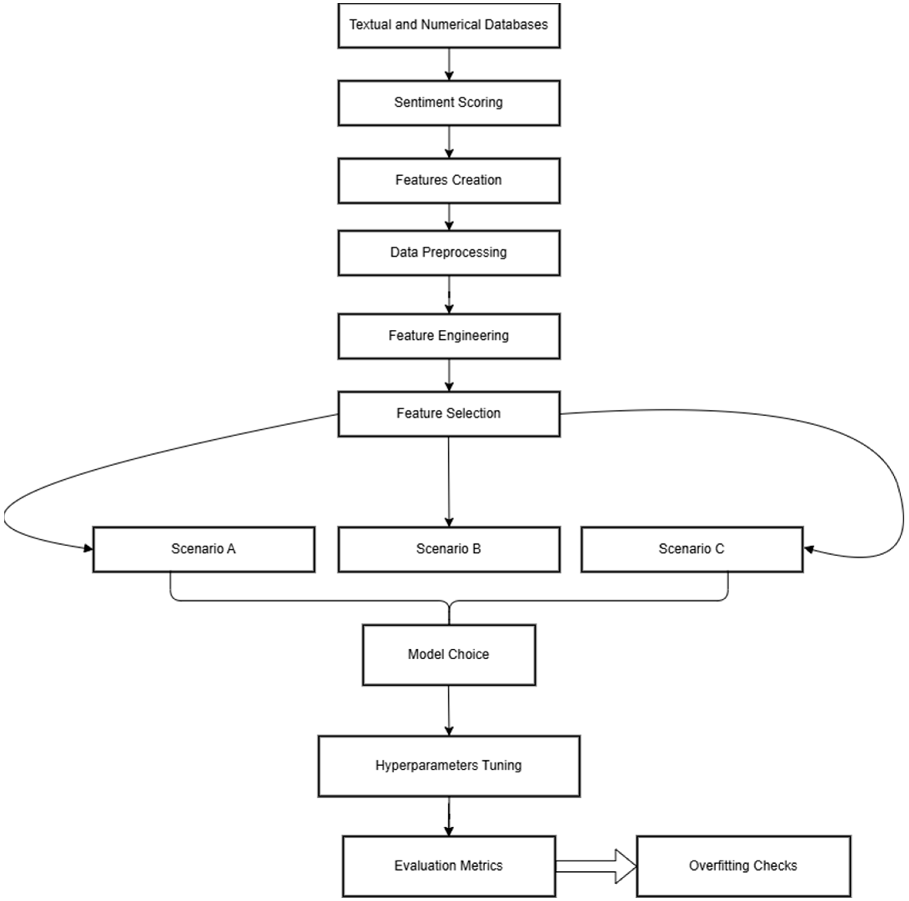
Accordingly, several ML models, namely LR, RF, GB, XGB Regressor, and MLP, were utilized to make predictions on S&P 500 index prices. Each of these models provides individual strengths in analyzing these factors for appropriate understanding of stock market movements. The visualization of this architecture is shown in Figure 1.

3.1. Data

The S&P 500 Index, or Standard and Poor’s 500, is an American stock market benchmark index composed of the 500 largest publicly traded companies listed on the U.S. stock exchange. Hence, it represents companies from all sectors, serving in that way as a gauge to the performance of the overall U.S. economy. Every movement in the index reflects the macroeconomic conditions of the wider economy and their corresponding microeconomic effect in different market sectors and its performance is indicative of investors’ confidence and changes during economic cycles, among other factors [44]. To secure the forecasting results from non-market historical events, we have utilized the daily adjusted closing price of the Index. This approach accounts for corporate actions such as dividends, stock splits, and rights offerings that would distort the index’s value over time.

Figure 2 presents the steps for generating the feature space and the final database scenarios. Both numerical and contextual data were retrieved from open access web sources, and various sentiment scoring methods, such as Textblob and pre-trained DistilBERT-base-uncased model were applied to generate the sentiment features. In a similar manner, using calculating methods for TA, the corresponding features were also generated. All features were preprocessed, standardized, and lagged accordingly to ensure computational efficiency.

The examination period in this study incorporates daily data of the Index, spanning from 2008 to 2016, and serves satisfactorily to reflect the larger reality of economic trends, as it incorporates a recovery phase following a financial crisis. During the crisis of 2008, the index experienced extreme turmoil that was mainly caused by the fall of the housing market and extensive problems within the financial sector. After plummeting to its lowest point in March 2009, the U.S. government began introducing economic stimulus to stabilize the financial markets with the help of low interest rates and other accommodative policies. These conditions strengthened the market, a process that was extended until 2015 and was characterized by significant gains for the S&P 500. In 2015, volatility of the prices resumed, mainly due to global concerns for the slowing economy of China and the uncertainty over oil prices, but not to such an extent as during the recession of 2008, which plummeted the index trend [45].

3.1.1. Sentiment Data

Daily headlines reflect public interest and sentiment toward major daily events happening globally, offering real-time context that often lines up with the markets’ reaction. In this study, sentiment data from Reddit World News is incorporated to offer a richer insight into the prediction process of the index. The data comprise the top 25 most upvoted daily headlines from subreddit World News, /r/worldnews, for the period between 8 June 2008 and 1 July 2015.

The strength of this dataset is its authenticity that is derived from the user-driven nature of Reddit to rank top headlines based on community engagement. On Reddit, users have options to upvote or downvote news posts, so only those that receive the most attention and attraction can climb the ranking lists. This key feature not only underlines critical world events but also reflects how important these events are perceived to be to the public. Sentiment analysis of the headlines, when scored and quantified, would therefore give a strong basis for measuring collective sentiment on dates and correlating it with stock market performance.

3.1.2. Macroeconomic Indicators

To capture the broader economic health in the US, a set of macroeconomic features that incorporate the view of individuals and policymakers indirectly in the US is employed along with a global macroeconomic index. The macroeconomic indicators of this study include the US 10-Year Treasury Bond Note Yield, the ISM Manufacturing PMI (PMI), the US Equity Market-related Economic Uncertainty Index, the Economic Policy Uncertainty Index (EPUI), the CEI, and the Business Confidence Index (OECD), offering a view that is both anchored in the cyclical business indicators themselves and responsive to sudden changes in economic uncertainty.

All indicators signal different aspects of the economic state that could influence S&P 500 price movements. More specifically, the US 10-Year Bond Yield is a proxy for long-term investor expectations about economic conditions and inflationary pressures. Expectations about the volatility of the market are also reflected in the Equity Market Uncertainty Index (EMUI), while EPUI epitomizes the level of uncertainty related to economic policy. An important measure of the attitude of consumers concerning their personal finance, business conditions, and economy, in general, is analyzed in CEI, while OECD BCI captures business managers’ opinions concerning output, new orders, and prospects of the global economic conditions. Lastly, PMI measures the strength of the manufacturing industry and hence it also provides a comprehensive overview of the economic and market conditions that drive performance in the S&P 500 [46,47,48,49,50]. Additional information of the indicators are provided in Appendix A.

3.1.3. Technical Analysis Indicators

Technical indicators are key components in predicting stock market movements that have been heavily used in the academic literature. While fundamental analysis makes estimates on the intrinsic value of a company, TA encompasses the study of the movement in prices and their patterns over time to predict future movements in the market. This paper examines the following five technical indicators: RSI, Stochastic Oscillator, Williams %R, EMA, and MACD.

Each of these indicators has its own strengths when it comes to suggesting the future performance of the S&P 500 through indications of momentum, overbought or oversold conditions, and trend direction. RSI is an indication that focuses on price momentum and mean reversion, while Stochastic Oscillator is one of the momentum indicators, which compares a certain closing price with its range for some period. Williams %R is also an oscillator that is used in this study and often gives indications of reversals well in advance of most other indicators. EMA is an indicator following trends that give more prominence to recent prices, while moving average convergence/divergence (MACD) embeds both trend following and momentum. With this set of indicators, dependency on any single indicator is reduced by providing a broad view of the market’s direction [51]. Additional information about the indicators is provided in Appendix B.

3.2. Data Engineering

In this subsection, a description of the basic data preprocessing is analyzed. Data were initially converted into a standard format for consistency and then redundant columns of the dataset were deleted. In addition, the data were merged and resampled to align different time series, while missing values were handled with appropriate imputation techniques to provide solid foundation for modeling and analysis.

Historical data from the S&P 500 index were downloaded by employing the yfinance library. The initial dataset included fundamental columns, such as Date, Open, High, Low, Close, Adj Close, and Volume over the period of analysis. The yfinance library is regarded as a respected source in the aggregation of stock market information, as its main source of information is Yahoo Finance. Hence, the use of the yfinance library indicates commitment to data reliability and efficiency, as the extraction would be through automated means, with no need for manual intervention. For this reason, the study would be guaranteed to operate on updated and complete historical data, an essential ingredient for accurate forecasting models.

Technical indicators provide major tools in financial analysis that one employs to quantify the stock price trends, momentum, and volatility. For the calculation of the indicators used in this study the ta.momentum library was employed. This library is ideal for the creation of such indicators, as it provides useful methods for capturing market dynamics. The library ta.momentum automates indicator calculations in a consistent manner that is error-free from complex indicators. This also enables the addition of technical indicators in the data, which contributes to identifying short-term patterns that may have a significant effect on the model’s performance.

Investor sentiment has nowadays become a key determinant of market fluctuations. Sentiment analysis techniques help to quantify the positive, neutral, or negative tone of news headlines that may influence stock prices. In this work, two methods have been implemented for calculating sentiment scores: TextBlob and pre-trained DistilBERT-base-uncased model from Hugging Face’s (HF) transformer library [52,53]. Advanced lexicon approaches and transformer-based pipelines like TextBlob and HF’s transformer library surpass other lexicon-based approaches like VADER, due to their deep linguistic and contextual analysis capabilities, when then are applied to lengthy or complex world news headlines. VADER and similar approaches perform better when they are applied to short texts found in X posts or short reviews as they are capable of capturing nuances like slang, emoticons, and intensifiers. VADER is suitable for short texts sentiment analysis as its ability to analyze longer, nuanced textual data is constrained [54].

Sentiment scores have been computed daily for 25 headlines related to world news. TextBlob is a lightweight library that uses the Natural Language Toolkit (NLTK) for sentiment analysis and is suitable at handling formal and structured language. Its methodology lays upon the idea of assigning for each text a polarity score, representing sentiment on a scale from −1 (negative) to 1 (positive) [52]. The average sentiment score of the headlines on each day has been computed from 25 daily headlines and gives a consolidated measure of the sentiment on a given day. Despite its simplicity, Textzblob library offers advantages against other libraries in processing and comparing the sentiments of news titles and descriptions [33].

In addition to Textblob library, the pre-trained DistilBERT-base-uncased model from HF transformers library was also employed to secure the effectiveness provided by Textblob and even more to enhance the results. This library gave access to a great number of pre-trained language models, enabling the comprehension of the meaning of news headlines. In contrast to TextBlob, that relies on a naïve polarity score, transformers-based models leverage DL models like BERT, RoBERTa, or DistilBERT to capture context, semantics, and nuances in text, making them ideal for complex texts, such as headlines. The daily average of the sentiment score was calculated in the same manner as in the case of TextBlob. Headlines with no string values were assigned with a 0-value indicating a rather neutral sentiment.

3.2.1. Cleaning and Converting the Data

Preprocessing the data was highly necessary in order to be able to have consistent and easily usable datasets. This first step was the conversion of the ‘Date’ column to ‘YYYY-MM-DD’ format. Next the renaming of column names was followed for better readability and to remove ambiguity. The columns ‘Open’, ‘High’, ‘Low’, ‘Close’, and ‘Volume’ were dropped as only daily adjusted closing prices with technical indicators and sentiments scores were used in the analysis.

3.2.2. Data Merging and Resampling

Merging data of different frequencies creates peculiar problems, especially when one merges daily and monthly datasets. Since technical indicators, sentiment scores, and most of the macroeconomic indicators were available at a daily frequency, they were combined directly into the daily adjusted closing price data of the S&P 500.

For some macroeconomic indicators, like the BCI, Consumer Confidence Index (CEI), and Purchasing Managers’ Index (PMI), that were available monthly, forward filling was used to incorporate them into a daily frequency dataset. This involved propagating the most recent monthly value forward to fill in the missing daily values throughout the month. This assumption is based on the idea that month-over-month indicators have fairly static effects during the month. It thus becomes suitable to use a forward-filling approach in capturing the daily stock price effect.

3.2.3. Handling Missing Values

Missing values can distort model accuracy and result in biased predictions when not properly treated. Columns that contained data errors, such as dots (.), were replaced with NaN to normalize these missing entries. Then, for these entries and for any remaining gaps, a rolling mean approach was implemented. This technique takes the average of the values, one before the others within a specified window for each missing value as its replacement. Such functionality removes spikes from this data and provides a much smoother time series on which to train a model.

Finally, for consistency purposes, the dataset was trimmed down to the period starting from 8 August 2008 up to 31 May 2016, considering availability for both market and sentiment data.

3.2.4. Feature Engineering

Feature engineering is the process of creating new input features to improve the learning and performance of a model. In this study, feature engineering was performed by lagging and standardizing key indicators to capture the temporal dependencies and avoid data leakage.

Lagging features is the process of bringing the values of the past forward to make new predictive inputs. This step helps the model identify temporal relationships and ensures that future data is not mistakenly used in predictions, preventing data leakage. In this study technical indicators were lagged for one day to show how their past values affect the immediate future market movements. Similarly, daily macroeconomic indicators were lagged by one day to ensure that only prior day data provides impact to the predictions preserving causal integrity. For monthly indicators, start-of-month and end-of-month values were resampled to a daily frequency. Each such value was then shifted by one month to account for its lagged effect. Finally, since news stories move markets very quickly, the sentiment scores were also lagged by one day so that it would give the models the context of sentiment on any previous day.

The StandardScaler method was used to standardize the features before model training as an important step toward best performance. This method transforms each feature by removing its mean and scaling it to unit variance. This scaler is then fitted directly on the training dataset to avoid data leakage and next is applied on both training and test datasets. Standard scaling of data is important in most ML models that are sensitive to the magnitude of features, especially those using gradient-based optimization methods. It allows most ML algorithms to operate optimally by making sure all features are given equal importance in the process of training, as it stabilizes numeric scale or range, increases the speed of convergence when training models, and ensures that each of the features is weighted equally in the learning process, particularly in models like LR, where unscaled features can distort coefficient estimates. Standardizing the data in this study ensures that input features are better utilized by all the models, therefore enhancing overall performance reliability.

3.2.5. Feature Selection

After generating and lagging features, the number of input features significantly increased. For this reason, RFE was selected to identify the most predictive features that would potentially make the models more efficient with increased performance. RFE is the technique that, with every iteration, takes away the least important features with regard to model performance until it finds the best subset of features that can be utilized for stock price prediction.

Feature ranking using the base model in this study was performed by applying this technique. As seen in

Table 1. Feature selection (Ranking).

Feature	Ranking
RSI_lag1	1
Stochastic Oscillator (%K)_lag1	1
Stochastic Oscillator (%D)_lag1	1
Exponential Moving Average (EMA)_lag1	1
MACD_Line_lag1	1
MACD_Signal_lag1	1
MACD_Diff_lag1	1
TB_Yield_10Y_lag1	1
Sentiment Score_Textblob_lag1	1
Sentiment Score_HF_lag1	1
BCI_lag1	2
ISM_PMI_lag1	3
CEI_lag1	4
William (%R)_lag1	5
EPUI_lag1	6
EMUI_lag1	7

, the features up to rank 2 were tested by the models and compared to the results produced by the models without considering this technique.

The aim was to reduce computational complexity and consequently avoid overfitting by removing uninformative or redundant features.

3.3. Descriptive Analysis

Descriptive statistics are major checkpoints in the analysis of the dataset, allowing an overview of its general characteristics. The dataset of this study spans from August 2008 to May 2026 and the statistical computations required, such as mean, median, variance, and standard deviation show the distribution of data, outliers, and possible errors in data entry. This initial overview of the target variable exhibits a mean that equals 1485.89 while the median is quite near to the mean value of 1385.22, both demonstrating an approximately symmetrically adjusted close price, with good support from the quite small value of the skewness that is equal to 0.138. The large value of standard deviation at 403.23 and large variance of 162,594 show that closing index prices have significantly varied and may probably be indicative of market volatility in the period under observation.

The technical indicators of the dataset show diverse behaviors, especially RSI, Stochastic Oscillator, and William %R. RSI has an average of 52.98, that is close to a neutral value of 50, with low skewness. For Moving Average and MACD, we obtain an EMA’s average that stands at 1483.26, relatively close to the average of the Adj Close and should therefore be a good signal of the trend direction. With regard to the sentiment scores, both sentiment indicators from Textblob and HF have average values close to zero, reflecting that overall, neutrality may be maintained in the dataset.

The macroeconomic indicators such as EPUI show large values for mean and variance, reflecting great uncertainty in economic policy. In contrast, the variable EMUI has a mean value of 49.49; therefore, it is much less volatile. ISM_PMI is one manufacturing indicator whose distribution is relatively balanced, with a mean of 52.56 and a moderate variance. This suggests the existence of moderate economic activity, without extreme changes. Additional information regarding the descriptive statistics, distributions of features, and scatterplots are presented in

Table A1. Descriptive statistics.

Variable	Mean	Median	Std	Variance	Skewness	Kurtosis	IQR	Min	25%	50%	75%	Max	Count
Adj Close	1485.89	1385.22	403.22	162,594.21	0.138	−1.275	729.98	676.53	1160.83	1385.22	1890.74	2130.82	1966
RSI	52.99	53.55	5.56	30.89	−0.51	0.22	7.89	33.96	49.52	53.55	57.41	65.73	1966
Stochastic Oscillator (%K)	67.92	76.26	28.7	824.1	−0.74	−0.62	46.2	0	47.04	76.26	93.25	100	1966
Stochastic Oscillator (%D)	67.89	76.01	27.9	778.92	−0.72	−0.71	46.012	0.77	46.87	76.01	92.88	99.79	1966
William (%R)	−37.87	−30.22	31.46	989.87	−0.49	−1.12	56.40	−100.00	−65.11	−30.22	−8.811	0.00	1966
Exponential Moving Avg (EMA)	1483.23	1385.39	401.04	160,830.45	0.151	−1.284	740.83	727.14	1164.18	1385.39	1905.01	2116.92	1966
MACD_Line	2.8	6.34	15.99	255.57	−1.598	3.79	18.07	−77.2	−3.89	6.34	14.179	32.13	1966
MACD_Signal	2.77	5.99	15.036	226.09	−1.59	3.66	16.98	−71.05	−3.488	5.99	13.49	28.63	1966
MACD_Diff	0.026	−0.035	4.88	23.86	−0.304	1.975	5.723	−26.649	−2.8	−0.035	2.919	18.29	1966
Sentiment_Score_Textblob	0.012	0.012	0.041	0.001	−0.0434	0.495	0.0533	−0.166	−0.014	0.012	0.038	0.197	1966
Sentiment_Score_HF	−0.574	−0.576	0.16	0.026	0.3	0.101	0.22	−0.98	−0.696	−0.576	−0.471	0.0748	1966
EPUI	117.02	100.3	71.376	5094.62	1.68	4.97	84.64	3.32	65.96	100.29	150.59	626.03	1966
EMUI	49.49	27.43	73.44	5394.62	5.555	50.95	45.15	4.80	11.99	27.43	57.13	1117.23	1966
TB_Yield_10Y	2.59	2.52	0.663	0.44	0.381	−0.99	1.09	1.43	2.02	2.52	3.11	4.08	1966
BCI	99.64	99.99	1.32	1.74	−1.93	3.24	0.88	95.27	99.55	99.99	100.43	101.24	1966
CEI	76.86	75.1	10.59	112.2	0.033	−0.69	14.2	55.3	69.9	75.1	84.1	98.1	1966
ISM_PMI	52.26	52.9	5.78	33.49	−1.36	2.22	5.7	32.4	50.2	52.9	55.9	61.40	1966

, and Figure A1 and Figure A2 in Appendix C.

Overall, the dataset reflects a mix of steady macroeconomic factors and more dynamic technical indicators. The stable sentiment indicators and macroeconomic indicators can outline the baseline for the long-term trend prediction, while technical indicators and EMA may capture short-run fluctuation. In addition, minimal skewness across most indicators suggests limited outliers, which could make for a good prediction model with less extensive data preprocessing or outlier treatment.

3.4. Modeling

In this study, five ML models were employed to predict a one-day lead time of the S&P 500 index price: LR, RF Regressor, GB Regressor, XGBoost Regressor, and MLP Regressor. While it is standard practice in time series forecasting to preserve the chronological order of observations in a train/test split, in this study, a random 20% of the data was set aside as a holdout test set for each distinct scenario, as detailed below. Lagged features were engineered to capture short-term temporal dependencies, such as previous-day values, and were included as model inputs.

To evaluate the impact of different feature combinations, the models were tested under three distinct scenarios:

(1)

All lagged features incorporated included only the sentiment score variable derived from pre-trained DistilBERT (Sentiment Score_pre-trained DistilBERT_lag1).

(2)

All lagged features incorporated including only the sentiment score variable derived from TextBlob (Sentiment Score_Textblob_lag1).

(3)

Only the features selected through RFE were incorporated up to level 2.

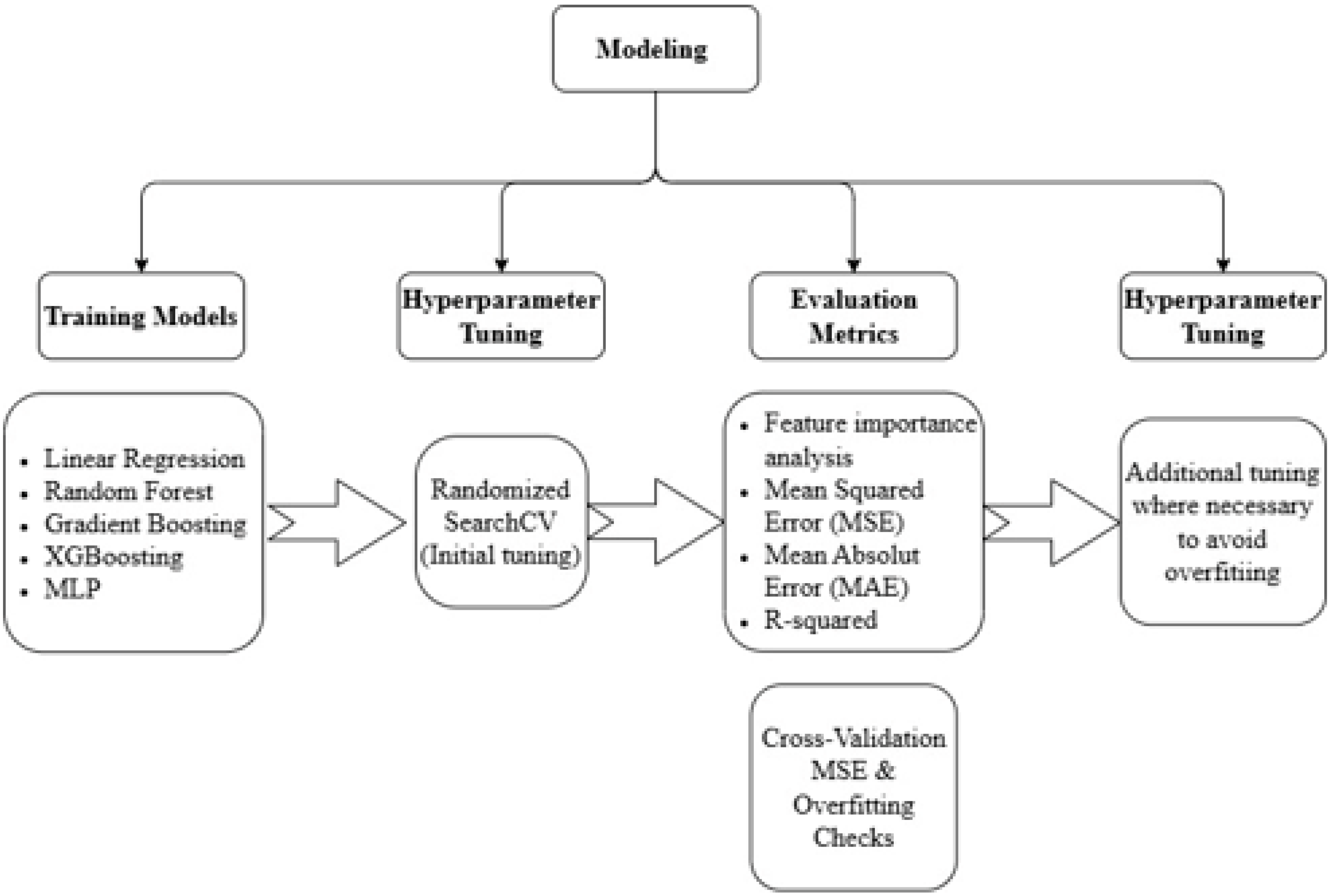
The dataset was then split into 80% for training and 20% for testing to facilitate unbiased model evaluation and ensure the generalizability of the results, as shown in Figure 3.

The hyperparameters of these models were initially optimized using RandomizedSearchCV, a method that randomly samples candidates from the hyperparameter space [55]. Computationally cheap, this approach generally yields comparable results to GridSearchCV, which performs an exhaustive search over a user-specified hyperparameter space [56]. Whereas GridSearchCV will ensure that the best configuration is found, this comes at a far higher computational cost. These techniques are important, as they allow models to find the optimal performance of the model by systematically testing and choosing the best hyperparameters for the data and the given task.

Since the models used in this study focus on the prediction of continues values and not categories, we evaluated their prediction error from the actual prices using MSE and MAE. In addition, R² was also a metric calculated in order to evaluate the proportion of the variance in the target variable that is explained by the model’s predictions. The purpose was to ensure that the tuning process was aligned with the goal of minimizing prediction error, while maximizing explanatory power. In addition, checks for overfitting were also employed using the Cross Validation (CV) technique and additional tuning to the hyperparameters of the models was made for those instances where overfitting was found.

Feature importance analysis was also conducted for all models to interpret the contribution of individual features to the predictions. This step is particularly useful in understanding what really drives the S&P 500 index price and thus provides insight into which technical, macroeconomic, or sentiment-based variables had greater predictive power. For ensemble models, such as RF and GB, feature importance was derived from the impurity or loss reduction attributed to each feature. Other models utilized coefficients or SHAP values to interpret feature contributions. Rigorous hyperparameter tuning and careful feature importance analysis boded well for models optimized for predictive accuracy, but also for being interpretable—a methodological alignment with the dual goals of robust forecasting and actionable insights.

3.4.1. Linear Regression

LR is considered a traditional model in ML which tries to capture the linear relationship between a set of input features and the target variable with an added bias term [57]. The simplicity and interpretability of the model makes it a good starting point for any predictive analysis [57].

Its simplicity makes it possible for quick implementation and forms the basis for understanding the relationship between features and the target variable. In this study, its interpretability was especially helpful in assessing the predictive power of technical, macroeconomic, and sentiment-based features. The coefficients allowed for quantification of the strength and direction of each separate feature’s influence on the price of the S&P 500 index. It also provided a baseline performance measure against the other models employed, since their outperformance signaled an indication that the relationship of the data is highly linear, and that the features engineering and data preprocessing are in order.

In this work, a Linear Regression model was constructed using the selected features for each scenario, with corresponding coefficients calculated, while the intercept term was enabled as specified by the function parameters. The implementation of LR was to fit the model on the scaled training dataset using the LinearRegression() class from Scikit-learn. The StandardScaler was applied to make all features be on a comparable scale, because unscaled data results in biased coefficient estimates in models sensitive to the magnitude of the predictors.

3.4.2. Random Forest Regressor

RF Regressor is a robust ensemble learning model that combines multiple trees to improve prediction performance and at the same time reduce overfitting [57]. Every tree in the forest is built on a random subset of data and features, using a method called bootstrap aggregation (bagging). This approach reduces the variance by averaging the prediction of each tree, thus resulting in a model that balances accuracy and generalization.

The choice of this model in the study is critical because of its ability to capture non-linear relationships and interactions between features, often prevalent in financial datasets [57]. Compared to other models, this makes no strong parametric assumptions, enabling the methodology to be more adaptive to high-dimensional and complex data. This flexibility is especially valuable given the diverse nature of the input features, since they all vary significantly.

In addition, the model’s resistance against overfitting allows for robust performance against the presence of noisy or less relevant predictors. By aggregating predictions from multiple trees, it mitigates potential overfitting to particular patterns in the training data which is common in financial modeling [57].

Hyperparameter tuning for the RF Regressor was carried out using RandomizedSearchCV. The choice of the parameter grid was made with consideration for model complexity, generalization, and computational efficiency. In the first effort, the hyperparameters provided by the RandomizedSearchCV resulted in overfitting signaling for additional tuning. To overcome overfitting, we further adjusted the maximum tree depth to 15, the minimum samples required to split a node to 10, and at least 5 samples per leaf, while estimators were reduced to 200.

These hyperparameters allow the RF Regressor to effectively learn the non-linear relationships in the data while avoiding overfitting. Hence, this combination was balanced enough to both be reasonably predictive, but also not overfitting for a good S&P 500 index price forecast.

3.4.3. Gradient Boosting Regressor

GB Regressor is an ensemble learning model that builds sequentially upon the weak learners (decision trees) in order to come up with a strong predictor. Each consecutive tree is trained to minimize the residual error of the previous tree using the gradient descent approach to optimize its loss function. This iterative approach ensures that the model focuses on instances that are difficult to predict, effectively shrinking bias and increasing accuracy [57].

Since non-linear relationships and feature interactions are usually present in financial data, employing such a model creates additional value in this study. Unlike simpler models, it uses additive corrections and, as a result, it is highly adaptive to the complexities of the dataset. This adaptability is very useful considering the diversity of the feature set that entails technical indicators, macroeconomic variables, and sentiment scores [57].

Another strength of GB is that, with proper tuning of the parameters, it can potentially be less biased and have a lower variance, hence generally being more resistant to overfitting. While this model has a greater propensity toward overfitting than RF, it can be regularized with different modifications in learning rate, limiting tree depth, and subsampling in order to minimize such risks [57].

The initial hyperparameter optimization for the GB Regressor was also made using RandomizedSearchCV with 5-fold cross-validation to make the evaluation robust. However, the choice for the parameter grid results in overfitting after employing the model; therefore, further tuning was made to secure minimum overfitting after training the model. Final hyperparameter tuning included 0.005 learning rate, max depth 3, max features 0.8, min samples leaf 4, samples split 10, 1000 estimators, subsample 0.8, random state 42 and max 10 iterations, after no improvement was observed in the validation score.

Given this hyperparameters tuning, complex patterns in the financial dataset are captured effectively by the GB Regressor. The sequential learning structure ensures a gradual reduction in bias, while the use of regularization parameters keeps the risk of overfitting low. Such characteristics make the GB Regressor a very apt candidate for the task of forecasting the S&P 500 index price, which needs to be highly generalized.

3.4.4. XGB Regressor

Extreme Gradient Boosting (XGB Regressor) can be considered an advanced ensemble model, which works on major principles of GB to enhance efficiency and performance. It trains the decision trees sequentially to minimize the residual errors of the previous iterations, using methods from gradient descent, optimization and boosting. Thus, combining these methods, the model is more efficient in reducing bias and controlling variance [58].

The key advantage of this model is that it is built to include regularization, parallelized learning, and optimized tree pruning which enhances its performance. The regularization technique is vital for the prevention of overfitting, even on high-dimensional data. By controlling the learning rate, limiting the depth of trees, and setting minimum thresholds for the child weight of a tree node, the model enforces generalization without losing any valuable accuracy. In addition, it introduces randomness in subsampling rows and columns while training, which makes XGBoost more generalized to unseen data [58].

The implementation of the model begins with some baseline prediction, which is usually the mean of the dependent variable. Iteratively, it computes residual errors, trains decision trees to minimize those residuals, and updates predictions by summing up weighted outputs of newly trained trees. Then, regularization is applied to adjust these weights during training and maintain generalization at good levels, avoiding overfitting at the same time. The accumulation of predictions from all trees yields the final output [58].

In this study, XGB Regressor has been selected due to its ability to capture complex, non-linear relationships within financial data. Hyperparameter tuning was again applied using RandomizedSearchCV with 5-fold cross-validation to ensure a robust evaluation. Overfitting was again evident in the results and additional hyperparameters tuning was conducted. In particular, final hyperparameters included a subsample rate = 0.8, estimators = 300, min_child_weight = 5, max_depth = 5, learning_rate = 0.01, colsample_bytree = 0.8, gamma = 0.1, reg_lambda (L2) = 1, reg_alpha (L1) = 0.5 to balance model sparsity and overfitting control, and random_state = 42 for reproducibility.

3.4.5. MLP Regressor

MLP Regressor is an NN based regression model that dynamically captures complex and non-linear relationships within data. Compared to other tree-based methods that partition data by splitting the features, this model processes input data through interconnected layers of neurons. Each neuron performs weighted transformations followed by non-linear activation functions that allow the model to approximate complex patterns and dependencies [57].

In addition, this model is also characterized by its flexibility to model various data distributions, especially for datasets with non-linear relationships between features, just like the case of this study since technical indicators, sentiment scores, and macroeconomic variables interact in unpredictable ways. It also incorporates regularization techniques, such as using L2 penalties, controlled through an alpha parameter, that can be helpful against overfitting by constraining model complexity. Lastly, the inclusion of activation functions like ReLU or tanh enables the model to adapt to varying data structures, enhancing its generalization [57].

Compared to the other models in this study, MLP Regressor provides an NN architecture that utilizes a layer of neurons directly to learn mappings between input and output instead of depending on decision trees to find patterns. This unique approach makes it especially powerful for scenarios in which the relationships among features are too complex or too subtle to be captured by traditional methods [57].

During the implementation of the model, the input space consists of scaled features. These inputs are fed through one or more hidden layers, where each neuron computes a weighted sum of inputs followed by a non-linear activation. The output layer produces a prediction for the regression problem in this study, and the model repeatedly updates its weights via a process termed ‘backpropagation’ that minimizes some predefined loss function. Regularization is used during training to achieve better generalization, and techniques like adjusting the learning rate also optimize the performance of the model [57].

As in previous models, hyperparameter tuning was initially applied using RandomizedSearchCV with 5-fold cross-validation to ensure a robust evaluation. Results were also checked for overfitting, with no significant evidence of important existence. The model was configured with 3 hidden layers, each containing 50 neurons, hidden_layer_sizes configuration = (50, 50, 50), regularization alpha = 0.001 and learning_rate_init = 0.01. The ReLU activation function was selected to handle non-linearity and prevent vanishing gradients while adam solver was used for efficient optimization.

The MLP Regressor is particularly suitable for financial modeling, since the technique operates admirably with high-dimensional data and allows for complex relationships between various predictors. The flexibility here complements the structured approach of tree-based models, providing a useful alternative to capture intricate patterns in financial datasets. This makes the method an integral component in building robust predictive models within the domain [43].

4. Results

In this section, the results per model are presented, after evaluating their performance using MSE, MAE, and R². In addition, feature importance results per model are also presented to determine the most valuable features contributing to the predictive power of the models. Lastly, a discussion follows regarding model overfitting evaluation, given additional metrics presented in

Table A2. Linear Regression (overfitting results).

Scenarios			Dataset Type	MSE	MAE	R2	Cross-Validation MSE
a	No-Feature Selection	Sentiment Score_pre-trained DistilBERT	Training	313.20	12.74	0.9981	323.21
			Test	370.05	13.79	0.9977
b	No-Feature Selection	Sentiment Score_extblob	Training	313.42	12.74	0.9981	324.71
			Test	371.03	13.84	0.9977
c	Feature Selection	Up to rank 2	Training	317.20	12.80	0.9980	326.98
			Test	375.19	13.88	0.9977

,

Table A3. Random Forest (overfitting results).

Scenarios			Dataset Type	MSE	MAE	R2	Cross-Validation MSE
a	No-Feature Selection	Sentiment Score_pre-trained DistilBERT	Training	60.75	5.76	0.9996	475.99
			Test	361.42	13.99	0.9979
b	No-Feature Selection	Sentiment Score_Textblob	Training	60.31	5.69	0.9996	488.40
			Test	378.09	14.26	0.9978
c	Feature Selection	Up to rank 2	Training	62.32	5.68	0.9996	480.65
			Test	371.78	13.73	0.9978

,

Table A4. Random Forest (overfitting results after additional tuning).

Scenarios			Dataset Type	MSE	MAE	R2	Cross-Validation MSE
a	No-Feature Selection	Sentiment Score_pre-trained DistilBERT	Training	318.41	13.07	0.9980	711.69
			Test	533.58	16.98	0.9969
b	No-Feature Selection	Sentiment Score_Textblob	Training	323.42	13.14	0.9980	722.92
			Test	540.30	17.27	0.9968
c	Feature Selection	Up to rank 2	Training	302.90	12.52	0.9981	771.25
			Test	556.94	17.15	0.9967

,

Table A5. Gradient Boosting (overfitting results).

Scenarios			Dataset Type	MSE	MAE	R2	Cross-Validation MSE
a	No-Feature Selection	Sentiment Score_pre-trained DistilBERT	Training	15.52	3.09	0.9999	458.13
			Test	524.65	16.22	0.9968
b	No-Feature Selection	Sentiment Score_Textblob	Training	14.81	3.01	0.9999	490.32
			Test	476.39	15.84	0.9971
c	Feature Selection	Up to rank 2	Training	15.28	3.07	0.9999	437.37
			Test	496.40	15.57	0.9970

,

Table A6. Gradient Boosting (overfitting results after additional tuning).

Scenarios			Dataset Type	MSE	MAE	R2	Cross-Validation MSE
a	No-Feature Selection	Sentiment Score_pre-trained DistilBERT	Training	261.98	12.17	0.9984	385.91
			Test	407.98	14.79	0.9975
b	No-Feature Selection	Sentiment Score_Textblob	Training	261.80	12.17	0.9984	386.21
			Test	408.05	14.80	0.9975
c	Feature Selection	Up to rank 2	Training	284.18	12.83	0.9982	419.06
			Test	424.83	15.16	0.9974

,

Table A7. XGB Regressor (overfitting results).

Scenarios			Dataset Type	MSE	MAE	R2	Cross-Validation MSE
a	No-Feature Selection	Sentiment Score_pre-trained DistilBERT	Training	25.29	3.94	0.9998	358.24
			Test	285.44	12.22	0.9983
b	No-Feature Selection	Sentiment Score_Textblob	Training	25.31	3.93	0.9998	359.21
			Test	287.20	12.26	0.9983
c	Feature Selection	Up to rank 2	Training	36.30	4.69	0.9997	366.90
			Test	300.40	12.52	0.9982

,

Table A8. XGB Regressor (overfitting results after additional tuning).

Scenarios			Dataset Type	MSE	MAE	R2	Cross-Validation MSE
a	No-Feature Selection	Sentiment Score_pre-trained DistilBERT	Training	728.51	21.59	0.9954	947.62
			Test	905.29	23.95	0.9947
b	No-Feature Selection	Sentiment Score_Textblob	Training	728.15	21.57	0.9955	948.27
			Test	908.73	23.97	0.9947
c	Feature Selection	Up to rank 2	Training	947.84	23.97	0.9941	1239.48
			Test	1159.31	26.65	0.9932

and

Table A9. MLP Regressor (overfitting results).

Scenarios			Dataset Type	MSE	MAE	R2	Cross-Validation MSE
a	No-Feature Selection	Sentiment Score_pre-trained DistilBERT	Training	359.66	14.52	0.9978	565.94
			Test	410.35	14.39	0.9976
b	No-Feature Selection	Sentiment Score_Textblob	Training	381.71	14.91	0.9976	593.18
			Test	413.13	15.50	0.9976
c	Feature Selection	Up to rank 2	Training	355.74	14.30	0.9978	451.50
			Test	336.53	13.90	0.9980

in Appendix D.

4.1. Linear Regression Findings

Following the implementation of the LR model, MSE, MAE, and R² were calculated to evaluate its performance for each one of the selected scenarios.

As per

Table 2. Linear Regression (results).

Scenarios			MSE	MAE	R2
A	No-Feature selection	Sentiment Score_pre-trained DistilBERT	370.05	13.79	0.9977
B	No-Feature selection	Sentiment Score_Textblob	371.03	13.84	0.9977
C	Feature selection	Up to rank 2	375.19	13.88	0.9977

, for the scenarios where feature selection was not applied, the model gave almost identical results regardless of the sentiment technique. Both MSE and MAE were almost identical, and with the high value of R², the model indicated that data are very well fitted, providing strong predictive power, regardless of the sentiment score employed. With feature selection applied, MSE slightly increased to 375.19 and MAE to 13.88, whereas R² remained high at 0.9977, demonstrating that while the model’s complexity was decreased when the input features were reduced to only the most important ones, there was not any significant loss in predictive capability.

After employing feature importance analysis, shown in

Table 3. Linear Regression (feature importance) scenarios.

	Scenarios
Feature	A	B	C
RSI_lag1	4.15	4.10	5.54
Stochastic Oscillator (%K)_lag1	28.71	28.72	30.68
Stochastic Oscillator (%D)_lag1	−25.40	−25.38	−27.19
William (%R)_lag1	1.65	1.68	n/a
Exponential Moving Average (EMA)_lag1	397.99	398.02	399.59
MACD_Line_lag1	4.48	4.47	4.64
MACD_Signal_lag1	0.48	0.48	0.40
MACD_Diff_lag1	12.96	12.93	13.73
EPUI_lag1	−1.67	−1.63	n/a
EMUI_lag1	−0.09	−0.14	n/a
TB_Yield_10Y_lag1	−2.96	−2.96	−2.10
BCI_lag1	−2.51	−2.42	−0.22
CEI_lag1	0.87	0.86	n/a
ISM_PMI_lag1	2.74	2.72	n/a
Sentiment Score_pre-trained DistilBERT_lag1	0.65	n/a	n/a
Sentiment Score_Textblob_lag1	n/a	0.45	0.52

, to interpret the contribution of each feature to model predictions, it was found that EMA_lag1 was the most influential feature for models without feature selection, with a value at 398. Stochastic Oscillator (%K)_lag1 and MACD_Diff_lag1, were also dominant in driving predictions, while both sentiment features had negligible effects, indicating that quantitative price-based patterns were more critical to index movement prediction. Using feature selection, EMA_lag1 remained dominant, with its importance increasing slightly to 399.59, while Stochastic Oscillator (%K)_lag1 and MACD_Diff_lag1 were still significant contributors, and sentiment-based features retained their marginal influence. This reduction in feature set size served well to emphasize the strong predictors, thus reassuring that this model concentrates on the important drivers without sacrificing accuracy. The Simple Linear Regression models established for each scenario can be found in Appendix E.

Residual analysis takes a closer look at the difference between actual and estimated values and therefore provides more detailed insights into model performance. Models without feature selection exhibited similar residuals between both sentiment sources. Most values fell between ±85, while the values at −4.93 and −4.96 presented good short-term predictions, and residuals with greater values, such as −85.40 and −84.72, presented challenges during extreme market changes. When feature selection was applied, residual patterns remained similar, with a few outliers, larger in some cases, like −87.76. However, the residual behavior remained quite similar to models without feature selection, showing feature selection does not much worsen model predictive accuracy. Hence, the model’s robustness and ability to maintain performance under varying configurations is evident. This is also evident in Figure 4, where the relationship between the actual and predicted values is presented.

The various evaluation metrics and analyses of feature importance bring out the resilience and effectiveness of the model. The minor rise in both MSE and MAE after feature selection demonstrates that the model can focus on the most relevant predictors without risking its performance. The dominance of technical indicators suggests their strong predictive power in capturing price trends and momentum, making them reliable inputs for the prediction of the index price. On the other hand, sentiment scores suggest that they are not capable enough to support the prediction of market movements. Overall, high R² indicates that the model explains almost all the variance in the index, and it is reliable and precise in stable market conditions.

4.2. Random Forest Regressor Findings

Following the LR results, the RF Regressor model was also trained to enhance predictive power. Initial results indicated slight differences across scenarios, with high R² and relatively higher errors compared to other models. As seen in

Table 4. Random Forest (results).

Scenarios			MSE	MAE	R2
A	No-Feature selection	Sentiment Score_pre-trained DistilBERT	533.58	16.98	0.9969
B	No-Feature selection	Sentiment Score_Textblob	540.30	17.27	0.9968
C	Feature selection	Up to rank 2	556.94	17.15	0.9967

, without feature selection, scenario A returned an MSE of 533.58, an MAE of 16.98, and an R² value of 0.9969, while scenario B yielded a slightly higher MSE of 540.3 and MAE of 17.27, though R² value remained high at 0.9968. With the refinement of features, scenario C resulted in an MSE marginally higher at 556.94, and decreased MAE of 17.15, indicating improved prediction accuracy. R² value declined slightly at 0.9967 but without affecting the robustness of the model. The results obtained in this instance suggest minimum usefulness of feature selection, since limiting features only to those which provide maximal insights had no significant impact to the overall model performance.

In addition to the initial evaluation, feature importance analysis was employed at this stage, providing further insights into the key drivers of the model, as per

Table 5. Random Forest (feature importance).

	Scenarios
Feature	A	B	C
Exponential Moving Average (EMA)_lag1	0.373	0.375	0.575
CEI_lag1	0.242	0.235	n/a
BCI_lag1	0.109	0.105	0.191
TB_Yield_10Y_lag1	0.091	0.095	0.149
EPUI_lag1	0.069	0.072	n/a
ISM_PMI_lag1	0.056	0.055	n/a
RSI_lag1	0.020	0.021	0.034
EMUI_lag1	0.015	0.016	n/a
MACD_Signal_lag1	0.010	0.009	0.022
MACD_Line_lag1	0.006	0.006	0.013
Stochastic Oscillator (%D)_lag1	0.004	0.004	0.004
Stochastic Oscillator (%K)_lag1	0.003	0.003	0.004
MACD_Diff_lag1	0.002	0.002	0.006
William (%R)_lag1	0.001	0.002	n/a
Sentiment Score_pre-trained DistilBERT_lag1	0.001	n/a	n/a
Sentiment Score_Textblob_lag1	n/a	0.001	0.002

. In all scenarios, (EMA)_lag1 was found to be the most influential feature as it accounted for almost 37% of the importance in scenario A and B, while in scenario C this value increased to 58%. Less important contribution was found in CEI_lag1 and BCI_lag1, but still relevant for the prediction task, while sentiment-based features proved to be the least important. Similarly, BCI_lag1 and TB_Yield_10Y_lag1 were found to have moderate contribution in scenario C, with the least impactful features to be the sentiment-based features.

Finally, residual analysis indicated the model’s strong prediction performance for all scenarios in Figure 5. In scenario A, residuals remained within reasonable bounds, except for some predictions where larger deviations were recorded, such as −31.35 and 27.96. The application of Sentiment Score_Textblob selection demonstrated a similar trend, as in scenario A, where residuals were found at −27.72 and 21.23. In scenario C, feature selection significantly improved the residual values, varying from −14.35 to 20.65. These results indicated reduced variability and closer alignment with the actual values. They also confirmed that key predictors have a significant impact on the model’s performance, when it refers to its capability of handling stable and dynamic market conditions with a reduced error margin.

4.3. Gradient Boosting Regressor Findings

After employing the GB algorithm, results provided negligible differences between the scenarios tested, as seen in

Table 6. Gradient Boosting (results).

Scenarios			MSE	MAE	R2
A	No-Feature selection	Sentiment Score_pre-trained DistilBERT	407.98	14.79	0.9975
B	No-Feature selection	Sentiment Score_Textblob	408.05	14.80	0.9975
C	Feature selection	Up to rank 2	424.83	15.16	0.9974

. For the no-feature selection scenarios sentiment Score_pre-trained DistilBERT scenario had an MSE of 407.98 and an MAE of 14.79 while sentiment score_Textblob scenario yielded a higher MSE of 408.05 and MAE of 14.80. Despite these differences, both models showed high R² values, underlining the model’s robust predictive power and capability to capture the underlying dynamics of the data. Employing the model after feature selection resulted in both MAE and MSE increasing to 15.16 and 424.83, respectively, while R² remained very high at 0.9974. Limiting features to the most relevant for building a model with high explanatory power proved that the overall accuracy of the predictions slightly deteriorated.

Next, feature importance analysis, shown in

Table 7. Gradient Boosting (feature importance).

	Scenarios
Feature	A	B	C
Exponential Moving Average (EMA)_lag1	0.801	0.801	0.883
CEI_lag1	0.146	0.146	n/a
BCI_lag1	0.032	0.032	0.090
ISM_PMI_lag1	0.010	0.010	n/a
TB_Yield_10Y_lag1	0.006	0.006	0.022
RSI_lag1	0.002	0.002	0.003
William (%R)_lag1	0.001	0.001	n/a
MACD_Diff_lag1	0.001	0.001	0.001
MACD_Line_lag1	0.000	0.000	0.000
Stochastic Oscillator (%K)_lag1	0.000	0.000	0.001
Stochastic Oscillator (%D)_lag1	0.000	0.000	0.000
MACD_Signal_lag1	0.000	0.000	0.000
EPUI_lag1	0.000	0.000	n/a
EMUI_lag1	0.000	0.000	n/a
Sentiment Score_pre-trained DistilBERT_lag1	0.000	n/a	n/a
Sentiment Score_Textblob_lag1	n/a	0.000	0.000

, indicated that EMA_lag1 was the most relevant feature for all scenarios, due to its significance in capturing price movement trends, with a value of 0.801 for both Sentiment Score_pre-trained DistilBERT and Sentiment Score_Textblob scenarios, respectively. Similarly, in the feature-selected model, EMA_lag1 dominated among the other features with a value of 0.883. With respect to the rest of the features, CEI_lag1 and TB_Yield_10Y_lag1 demonstrated moderate importance, while sentiment-based features exhibited even lower importance.

With regard to the residual analysis, it was found that residuals were mainly between acceptable bounds with some variation in instances depending on either the sentiment score or the feature selection. Without feature selection, residuals using Sentiment Score_pre-trained DistilBERT were at −21.50 in one instance, while slightly higher predictive error was noticed when using Sentiment Score_Textblob, as the value was −33.32. Feature selection generally resulted in improved residual behavior. Deviations between the actual and predicted values became smaller. For instance, the residual of −6.79 in the feature-selected model is smaller compared to larger deviations in models without feature selection. Yet, even with such improvements, all models show excellent performance in stable market conditions but reveal their limitations during volatile or extreme periods. Figure 6 also confirmed the predictive power of the model against the actual values.

4.4. XGBoost Regressor Findings

XGBoost Regressor also provided high accuracy results for all scenarios, with minor variations stemming mainly from the feature engineering strategy shown in

Table 8. XGBoost Regressor (results).

Scenarios			MSE	MAE	R2
A	No-Feature selection	Sentiment Score_pre-trained DistilBERT	905.29	23.95	0.9947
B	No-Feature selection	Sentiment Score_Textblob	908.73	23.97	0.9947
C	Feature selection	Up to rank 2	1159.31	26.65	0.9932

. For no feature selection scenarios, employing the Sentiment Score_Textblob feature resulted in an MSE of 908.73, an MAE of 23.97, and R² of 0.9947. Instead, adopting Sentiment Score_pre-trained DistilBERT feature in the model resulted in an MSE of 905.29, an MAE of 23.95, and an R² of 0.9947. Employing only the features as suggested by RFE resulted in a minor effect on the performance of the model, as MSE increased to 1159.31 and MAE to 26.65, while R² slightly decreased to 0.9932.

In the next step of feature importance analysis, shown in

Table 9. XGBoost (feature importance).

	Scenarios
Feature	A	B	C
CEI_lag1	0.482	0.481	n/a
Exponential Moving Average (EMA)_lag1	0.273	0.273	0.653
BCI_lag1	0.071	0.071	0.164
ISM_PMI_lag1	0.051	0.052	n/a
TB_Yield_10Y_lag1	0.043	0.043	0.097
EPUI_lag1	0.037	0.035	n/a
MACD_Signal_lag1	0.012	0.013	0.028
EMUI_lag1	0.011	0.012	n/a
RSI_lag1	0.010	0.010	0.030
MACD_Line_lag1	0.005	0.005	0.018
Stochastic Oscillator (%D)_lag1	0.003	0.003	0.005
Stochastic Oscillator (%K)_lag1	0.001	0.001	0.002
William (%R)_lag1	0.001	0.001	n/a
MACD_Diff_lag1	0.001	0.001	0.002
Sentiment Score_pre-trained DistilBERT_lag1	0.000	n/a	n/a
Sentiment Score_Textblob_lag1	n/a	0.000	0.001

, CEI_lag1 was found to be the most important predictor in the models trained so far in the first two scenarios. In particular, the feature contributed more than 48% to the model’s importance for scenarios A and B, while other variables, such as (EMA)_lag1, ISM_PMI_lag1, and BCI_lag1, had a relatively minor contribution. In the feature selection scenario, EMA_lag1 importance increased up to 65%, reflecting the model’s reliance on this technical indicator. Features like TB_Yield_10Y_lag1and RSI_lag1 increased their importance weight after feature selection, supporting their impact in prediction accuracy improvement.

In residual analysis, the model’s accuracy is further confirmed in Figure 7. Without feature selection, scenarios are characterized by small variations in residuals, ranging between −10.59 and 19.31, thus capturing reasonable accuracy market trends. In the feature selection scenario, residuals kept this trend, as minimal deviations from actual values were reported raging between −0.19 and 14.55.

4.5. MLP Regressor Findings

The last model employed in this study was MLP Regressor. Similar to the results of the other models, minor variations in accuracy were estimated, depending mainly on the use of feature selection and sentiment score sources, as seen in

Table 10. MLP Regressor (results).

Scenarios			MSE	MAE	R2
A	No-Feature selection	Sentiment Score_pre-trained DistilBERT	410.35	14.39	0.9976
B	No-Feature selection	Sentiment Score_Textblob	413.13	15.50	0.9976
C	Feature selection	Up to rank 2	336.53	13.90	0.9980

. No feature selection scenario A achieved an MSE of 410.35, an MAE of 14.39, and an R² of 0.9976. In scenario B, MSE and MAE were found at 413.13 and 15.50, respectively, with an improved R² of 0.9976, reflecting an even better fit and stronger ability to capture the underlying data patterns. The model continued to perform well with feature selection criteria, as MSE was found at 336.53, MAE at 13.90, and R² at 0.9980. This approach, while slightly more accurate, streamlined the model and improved computational efficiency.

The analysis of the feature importance shown in

Table 11. MLP Regressor (feature importance).

	Scenarios
Feature	A	B	C
Exponential Moving Average (EMA)_lag1	1.831	1.778	1.847
MACD_Signal_lag1	0.008	0.006	0.027
BCI_lag1	0.008	0.005	0.004
Stochastic Oscillator (%K)_lag1	0.007	0.006	0.011
Stochastic Oscillator (%D)_lag1	0.007	0.008	0.009
ISM_PMI_lag1	0.005	0.011	n/a
TB_Yield_10Y_lag1	0.004	0.005	0.003
MACD_Diff_lag1	0.003	0.001	0.001
CEI_lag1	0.003	0.004	n/a
EMUI_lag1	0.002	0.000	n/a
RSI_lag1	0.002	0.003	0.006
William (%R)_lag1	0.002	0.001	n/a
MACD_Line_lag1	0.002	0.003	0.035
EPUI_lag1	0.001	0.000	n/a
Sentiment Score_pre-trained DistilBERT_lag1	0.000	n/a	n/a
Sentiment Score_Textblob_lag1	n/a	0.000	0.000

indicated that EMA_lag1 dominated among all scenarios, with an importance score between 1.778 and 1.847, making it again the most critical feature in the prediction. Secondary features with an adequate importance to the model were Stochastic Oscillators, BCI_lag1, and MACD_Signal_lag1. Sentiment scores had minor positive effects that added minor context for improving overall accuracy. During feature selection, lower-relevance variables, including ISM_PMI_lag1 and William (%R)_lag1, were excluded so that the model focuses only on impactful predictors.

Model accuracy was also evident in residual analysis. Most of the residuals exhibited minimal deviation, suggesting high predictive power between the actual values and their corresponding predictions. In scenario A, without feature selection, residuals ranged from −22.48 to 21.91 while in scenario B from −19.04 to 13.46, reflecting the superior alignment of the predicted values. The feature selection scenario exhibited similar residual variation but emphasized the model’s reliance on fewer, yet impactful predictors. The strong predictive power of the model is presented in Figure 8.

5. Discussion

In this study, we aimed to predict the daily S&P 500 adjusted closing price, based on a diverged set of input features by employing a spectrum ranging from simple to advanced ML techniques. The combination of technical, macroeconomic, and sentiment indicators was introduced in three different scenarios in order to reflect the insight of price trends, broader economic conditions and behavioral dimension into the market’s price movements. While prior studies have utilized relative features to forecast market trends, immediate comparison with the dataset examined in this study is not possible. The novelty of this study is the incorporation of macroeconomic variables that are neither examined in isolation nor combined with other TA and sentiment factors in the literature. In addition, DistilBERT-base-uncased model has not been found in relevant prior studies for calculating sentiment scoring, thus it can be inferred that an immediate comparison is not possible, since no prior research has used the same data.

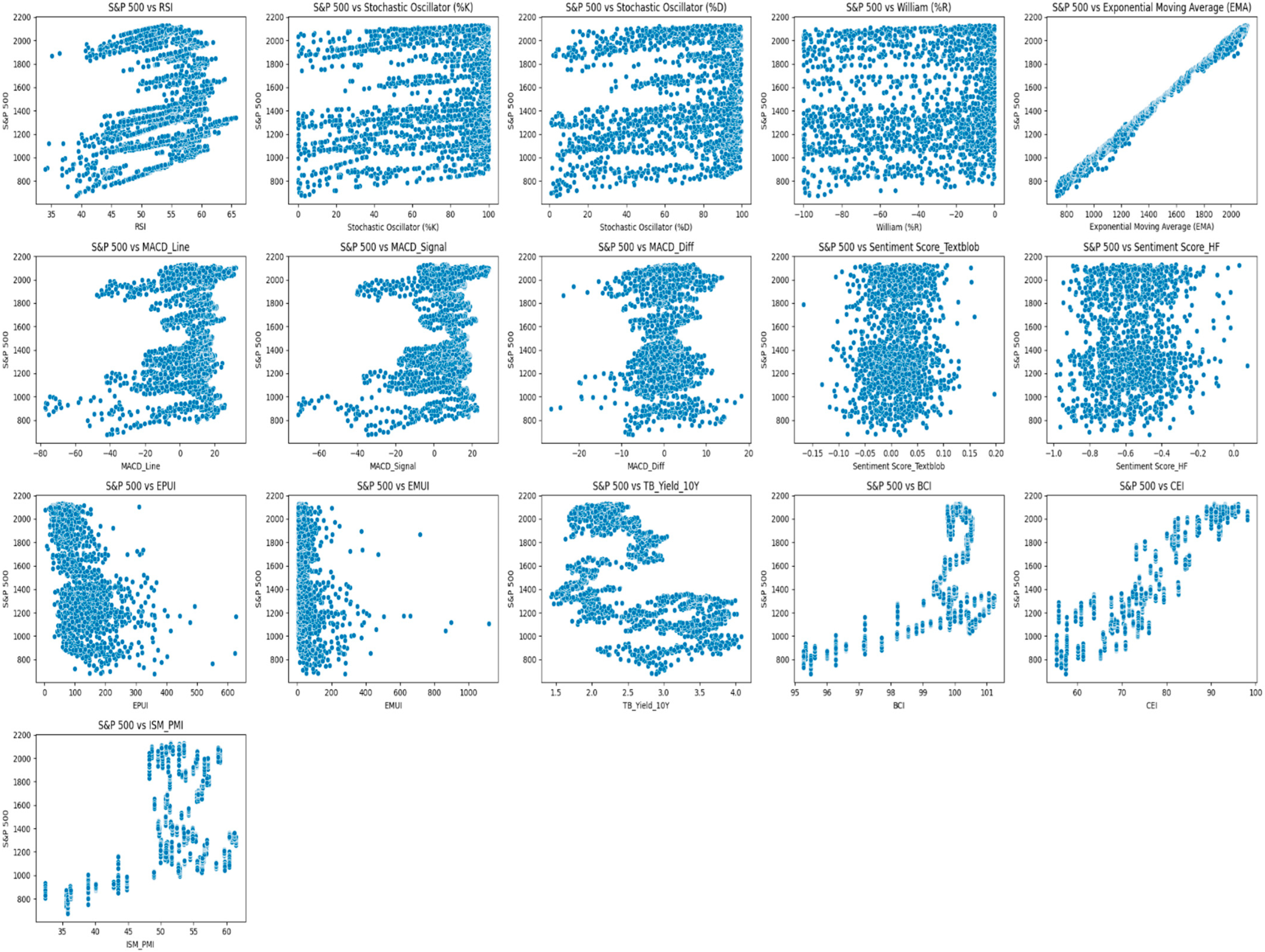
Results indicated a distinct relationship of these features in explaining their ability to predict the market. Initially, sentiment features were found to have a negligible contribution, suggesting a significant low impact to drive short market fluctuations. Macroeconomic features, while being a mirror of the economic conditions, produced subdued effects in short-term predictions, partially explained by their lagging nature and the daily prediction frequency. On the other hand, technical features related to momentum and volatility were found to contribute significantly, aligning with the TA theory that supports their ability to capture periods of overreaction and correction in financial markets.

In terms of the models’ predictive power, all models were found to provide a perfect fit, thoroughly explaining the variability of the input features in the S&P 500 price for all case scenarios. LR and MLP were the drivers among all models, providing high R² and low errors, supporting the concept that traditional and more advanced models can provide comparable results. MLP was found to better capture the dependencies found in scenario C, where features were defined by RFE. Similar results were also found in other models, but overfitting was evident, even after the additional tuning of the initial architecture of the hyperparameters provided by the RandomizedSearchCV technique.

While these findings indicate that the combination of these features can perfectly predict index price movements, further balance between model complexity and generalizability is also evident. Despite the efforts towards mitigating overfitting, such as hyperparameter tuning, cross-validation, and feature selection using RFE, to draw more robust conclusions about the interplay between features and their contribution to market predictions, RF, GB and XGB Regressor were found to be not reliable.

In all, this analysis leads to the conclusion that stock market behavior is so complex that no single variable acts dominantly. The integration of technical, macroeconomic, and sentiment data provides a comprehensive perspective, but also brings out the requirement for rigorous preprocessing and thoughtful choice of modeling strategies. While predictive accuracy can be realized, the nuanced interactions between variables continue to be a limiting factor for financial time series forecasting.

5.1. Benchmarking Results Against Literature

The aim of this study was to challenge and further enhance the predictive power of the models employed in the literature in the scope of finding the optimal feature combination to predict the stock market. In addition, the different methodological-based approaches (linear, tree-based, DL), aimed to assess the performance with different architecturally designed models. While each study addresses distinct aspects of forecasting stock prices, the focus of this subsection is to highlight the limitations that this work aimed to overcome.

Sangeetha and Alfia (2024) and the current work share the objective of predicting the S&P 500 index but differ in their methodology [8]. In their study, they use basic stock market features (Open, Close, Low, High, Volume) and implement the Evaluated Linear Regression-based ML (ELR-ML) technique, achieving an R² of 0.428 and an Adjusted R² of 0.352. Error metrics in their study show an SSE of 6 × 10¹³ and an MSE of 9 × 10¹², suggesting higher prediction deviations. In contrast, the models in this study achieved R² values nearing 0.998 and much lower errors, with an MSE as low as 261.98 for GB, underscoring the advantages of diverse features and sophisticated models. While in their study they employ a simple feature set that limits its ability to capture complex market dynamics, our study’s integration of richer data sources improves accuracy significantly. This limitation highlights the weakness of LR to explain non-linear financial data, while the advanced algorithms of this study can excel with proper feature engineering. Combining our study’s diverse features with Sangeetha and Alfia (2024)’s [8] residual analysis could refine both methodologies, emphasizing the importance of robust features and advanced techniques for accurate stock market forecasting.

Prime (2020) has also implemented LR and additionally NN in order to predict the stock price movements in Shanghai Stock Exchange using 21 indicators, categorized into macroeconomic, microeconomic, sentiment, and institutional investor data [43]. In their study they found that NN generally outperformed Regression models supported by p-values ranging from 0.08 to 1.00 for paired t-tests, with NN showing lower APE in most sectors. While their work suggested the superiority of NN models against basic regression models, their improved ability is not that evident in sectors with lower volatility. The sophisticated models in our study offer the ability to handle non-linear relationships more effectively, possibly explaining their higher predictive accuracy compared to both NN and OLSR in Prime (2020) [43].

The study from Jabeur et al. (2024) utilizes various ML models differentiating significantly from our work in their feature sets and target variables [39]. Both studies highlight the effectiveness of XGBoost in forecasting financial data when various input variables are utilized. In Jabeur et al. (2024) [39], XGBoost achieved the highest R² of 0.994 with RMSE of 34.921 and MAE of 21.968, showing strong accuracy in forecasting gold prices similar to the R² of 0.998 of our study. While errors were significantly lower than in our study for XGBoost and the other models (NN RMSE 195.961, LR RMSE 71.325), the advantage of ensemble models is evident in both studies, highlighting the importance of advanced algorithms for complex market data.

Compared to more advanced NN architectures studies in the literature, our study demonstrates the advantage of combining various features for broader market forecasting and, at the same time, the disadvantage of higher errors obtained when simpler models are implemented. In particular, Agrawal et al. (2019) [6] employ deep NN (Optimal LSTM and ELSTM) to predict banking stock prices using only technical indicators. Their results show superior performance with high accuracies in prediction of 63.59% for HDFC, 56.25% for YES Bank, and 57.95% for SBI, surpassing classical models like SVM and Logistic Regression that were also tested and ranged between 49% and 56% accuracy. In addition, the obtained MSEs for deep NN model were found at 0.015 and 0.017, being significantly lower than our study’s results [6]. While deep NN models performed significantly better in terms of error measurement, the importance of leveraging diverse features for a more comprehensive market analysis, as shown in our study, could be considered complementary to enhance the models.

Additional work that supports this novelty is further found in Chang et al. (2024), where they predict individual stock prices after employing DL models, such as GRU and LSTM, on their temporal dependencies and achieve an RMSE as low as 3.43 for Apple and 8.08 for Microsoft, significantly outperforming traditional methods [7]. In addition, Bhandari et al. (2022) employ LSTM models with different neuron configurations in order to predict the S&P 500 price using a combination of fundamental, macroeconomic, and technical indicators and report RMSE values ranging from 46.5 to 167.5 and high R² values between 0.9935 and 0.9967 [40].

5.2. Threats to Validity and Limitations

Despite the valuable insights of this study, there are still a few limitations. The first threat to validity of this study is linked to the selected indicators. Even though the selected technical and macroeconomic variables vary among their inferences, it is possible that other influential variables, such as sectoral metrics or global economic indicators, which could have greater contribution in forecasting, might have been left out. Not incorporating such a feature in the dataset could negatively affect the strength of the models in capturing stock market dynamics.

Secondly, the decision to incorporate macroeconomic indicators that calculate monthly values and lag them by one month raises questions about their temporal relevance. Economic conditions are generally reflected in the market over longer or variable time frames, and a uniform one-month lag may not adequately capture their effect. Similarly, lagging all other technical and macroeconomic indicators by one day may have constrained the analysis further, since they might require longer periods of lagging in order to reflect their impact accurately.

Forward-filling of monthly macroeconomic data is another threat in this research. While this approach is simple and effective to handle data, it can reduce model accuracy. In this study, forward-filling assumes that monthly values reflect the preceding days of the month, and this could potentially misrepresent trends or variations that could influence the market. Additionally, we acknowledge that a randomly selected sample of the test set does not immediately reflect real-world forecasting scenarios, as the test set is not exclusive to future data. As such, this evaluation should be interpreted as an exploratory assessment of model performance rather than a strict simulation of real-time forecasting.

Moreover, the scope of the sentiment analysis in this study is based on the effect of general world news on market price conditions. The open economic market that we reside in has set strong dependencies among countries, industries, and companies in order to achieve economic growth and development. The US economy is dominant worldwide and therefore companies that are incorporated in the S&P 500 can be heavily affected by world developments. While the focus in this study was to deviate from the usual implementation of examining sentiment from financial news and utilize the potential of highlighting the impact of world news on stock market movements, no significant relationship was found. A possible reason for this limitation could be the source and magnitude of the data retrieved from Reddit. As discussed in the data section, earlier data for sentiment retrieved from /r/worldnews can be considered a narrow perspective on market sentiment, as it does not particularly focus on world events relevant to business outcomes and may include information irrelevant to market impact. In order to provide a more detailed base of the behavior in the market, this could be further enriched by a more targeted source, such as business news or relevant social media.

In addition, another limitation of this study is that models were applied to historical data. While TA and macroeconomic indicators can be retrieved and applied in real time in the models, this is not possible for contextual data. Sentiment analysis would require specific setups for the retrieval and forecasting pipelines; hence, this is a limitation for live application of this research.

Furthermore, another limitation could be related to feature collinearity. For instance, RSI, EMA, and MACD are computed using overlapping calculations, which might induce redundancy and decrease the marginal contribution of each variable. This might affect the interpretability and the predictive performance of the model, thus requiring a more thorough selection and evaluation process.

These limitations highlight the complexity of financial forecasting and the trade-offs inherent in data preparation and modeling choices. These challenges call for the thoughtful refinement of methods and assumptions in future studies.

6. Conclusions and Future Work

The ability to predict stock market movements has always been of great importance in financial research and practice, due to the potential that it provides for investors, financial analysts, and policymakers to improve their decisions and manage risks. The aim of this study was to develop a comprehensive framework of financial modeling that integrates various input features, such as technical indicators, macroeconomic variables, and sentiment scores as predictors that can address the challenges that come with forecasting stock prices.

The practical application of the forecasting techniques proposed by this study could offer valuable insights for interested parties, such as investors, to adjust financial portfolio’s allocation, by alerting for potential short-term losses or enhanced short-term returns. Policymakers could also benefit from the model’s application by the long-term warning signals of turmoil in the markets, so that they could proactively act with changes in monetary or fiscal policy.

The financial modeling developed in this study utilizes ML regression models, including LR, RF, GB, XGBoost, and MLP, that aims to investigate how these factors combined can eventually provide better effectiveness in predicting the daily adjusted closing price of the S&P 500 index. Results suggest useful insights into the predictive power of different feature combinations, and the comparative performances of different ML models in this context.

One of the contributions of this study is that it introduces macroeconomic indicators into the forecasting architecture, in addition to more commonly used technical and sentiment-based features. Given the preprocessing steps and the feature engineering procedure as parts of the overall architecture, variables were lagged appropriately, indicating EMA and MACD as the features with the highest contribution. Macroeconomic factors, such as the BCI and CEI, were able to modestly explain market trends, confirming technical indicators’ established relevance for financial forecasting and modeling in the literature. For additional information, sentiment scores were computed using TextBlob and HF tools, but their contribution in this study was proved negligible.

Based on the feature dataset chosen for this study, modeling architecture exploits the effectiveness of various traditional and more advanced ML models to capture complex and non-linear relationships hidden in stock market data. Among the models tested, LR and MLP Regressor exhibited superior performance, achieving high R² scores of 0.99 and low MSE and MAE rates averaging 350 and 13 points, respectively, across both training and test datasets. Additional techniques for robust feature selection, such as RFE, were also utilized, slightly improving model efficiency in terms of error prediction, as predictive accuracy was already high. However, challenges, such as overfitting found in other models, underscore the importance of careful hyperparameter tuning and cross-validation techniques to enhance generalizability.

While the results of this study indicate important implications for investors to identify market trends and for researchers to further explore hybrid models combining various sets of features with modern ML techniques, limitations are also evident, possibly threating the validity of the results. Shortcomings related to the choice of macroeconomic indicators, the lagging timeframe of features and resampling, the nature and quality of contextual data, the inability to use build up and pipelines for live sentiment analysis, and the possible collinearity of technical indicators can significantly challenge the credibility of the results.

In conclusion, this study aims to add value to the existent literature to understand stock market predictions dynamics by incorporating the macroeconomic factor in ML models. Despite its possible limitations, actionable findings that serve as a strong base can be identified to contribute to the growing field of financial forecasting.

Future Work

Implications for future work to enhance the robustness of the models for stock price predictions are evident. Additional metrics that reflect particular sectors of the market and macroeconomic conditions can enhance the prediction power of the models, while alternative sources to broaden the scope of sentiment analysis in order to capture behaviors from financial news social media discussions could strengthen financial modeling.

In addition, applying optimized methods like rolling window regression, transfer entropy, etc., to assess the optimal lag periods for the macroeconomic indicators could be vital for explaining market prediction. Similarly, the investigation of alternative imputation techniques for monthly data may reduce the risks associated with forward-filling and improve data fidelity.

Finally, Principal Component Analysis or feature selection through clustering could also be employed to avoid feature collinearity and improve model interpretability and performance [59]. By addressing these issues, further work can build on the ground prepared by this study and advance financial modeling to produce more actionable insights.

References

1. Sonkavde, G.; Dharrao, D.S.; Bongale, A.M.; Deokate, S.T.; Doreswamy, D.; Bhat, S.K. Forecasting Stock Market Prices Using Machine Learning and Deep Learning Models: A Systematic Review, Performance Analysis and Discussion of Implications. Int. J. Financ. Stud. 2023, 11, 94. [Google Scholar] [CrossRef]
2. Mehrkian, S.S.; Davari-Ardakani, H. An Integrated Model of Sentiment Analysis and Quantitative Index Data for Predicting Stock Market Trends: A Case Study of Tehran Stock Exchange. Expert. Syst. Appl. 2025, 269, 126298. [Google Scholar] [CrossRef]
3. Shahi, T.B.; Shrestha, A.; Neupane, A.; Guo, W. Stock Price Forecasting with Deep Learning: A Comparative Study. Mathematics 2020, 8, 1441. [Google Scholar] [CrossRef]
4. Zhou, X.; Zhou, H.; Long, H. Forecasting the Equity Premium: Do Deep Neural Network Models Work? Mod. Financ. 2023, 1, 1–11. [Google Scholar] [CrossRef]
5. Hu, M.; Tang, Z.; Xie, X.; Jiang, M. Stock Prediction and Analysis Based on Support Vector Machine. Front. Bus. Econ. Manag. 2022, 5, 98–101. [Google Scholar] [CrossRef]
6. Agrawal, M.; Khan, A.U.; Shukla, P.K. Stock Price Prediction Using Technical Indicators: A Predictive Model Using Optimal Deep Learning. Int. J. Recent Technol. Eng. 2019, 8, 2297–2305. [Google Scholar] [CrossRef]
7. Chang, V.; Xu, Q.A.; Chidozie, A.; Wang, H. Predicting Economic Trends and Stock Market Prices with Deep Learning and Advanced Machine Learning Techniques. Electronics 2024, 13, 3396. [Google Scholar] [CrossRef]
8. Sangeetha, J.M.; Alfia, K.J. Financial Stock Market Forecast Using Evaluated Linear Regression Based Machine Learning Technique. Meas. Sens. 2024, 31, 100950. [Google Scholar] [CrossRef]
9. Papageorgiou, G.; Gkaimanis, D.; Tjortjis, C. Enhancing Stock Market Forecasts with Double Deep Q-Network in Volatile Stock Market Environments. Electronics 2024, 13, 1629. [Google Scholar] [CrossRef]
10. Koukaras, P.; Nousi, C.; Tjortjis, C. Stock Market Prediction Using Microblogging Sentiment Analysis and Machine Learning. Telecom 2022, 3, 19. [Google Scholar] [CrossRef]
11. Koukaras, P.; Tsichli, V.; Tjortjis, C. Predicting Stock Market Movements with Social Media and Machine Learning. In Proceedings of the International Conference on Web Information Systems and Technologies, WEBIST—Proceedings, Online, 26–28 October 2021. [Google Scholar]
12. Nousi, C.; Tjortjis, C. A Methodology for Stock Movement Prediction Using Sentiment Analysis on Twitter and StockTwits Data. In Proceedings of the 6th South-East Europe Design Automation, Computer Engineering, Computer Networks and Social Media Conference, SEEDA-CECNSM 2021, Online, 24–26 September 2021. [Google Scholar]
13. Fama, E.F. The Behavior of Stock-Market Prices. J. Bus. 1965, 38, 34. [Google Scholar] [CrossRef]
14. Fama, E.F. Efficient Capital Markets: A Review of Theory and Empirical Work. J. Financ. 1970, 25, 383. [Google Scholar] [CrossRef]
15. Edwards, R.D.; Magee, J.; Bassetti, W.H.C. Technical Analysis of Stock Trends; CRC Press: Boca Raton, FL, USA, 2012. [Google Scholar]
16. Rhea, R. The Dow Theory: An Explanation of Its Development and an Attempt to Define Its Usefulness as an Aid in Speculation. Am. Econ. Rev. 1933, 23, 252. [Google Scholar]
17. Kendall, M.G.; Hill, A.B. The Analysis of Economic Time-Series-Part I: Prices. J. R. Stat. Soc. Ser. A 1953, 116, 11. [Google Scholar] [CrossRef]
18. Bing, L.; Chan, K.C.C.; Ou, C. Public Sentiment Analysis in Twitter Data for Prediction of a Company’s Stock Price Movements. In Proceedings of the Proceedings—11th IEEE International Conference on E-Business Engineering, ICEBE 2014—Including 10th Workshop on Service-Oriented Applications, Integration and Collaboration, SOAIC 2014 and 1st Workshop on E-Commerce Engineering, ECE 2014, Guangzhou, China, 5–7 November 2014. [Google Scholar]
19. Cakra, Y.E.; Distiawan Trisedya, B. Stock Price Prediction Using Linear Regression Based on Sentiment Analysis. In Proceedings of the ICACSIS 2015—2015 International Conference on Advanced Computer Science and Information Systems, Proceedings, Malang, Indonesia, 15–16 October 2016. [Google Scholar]
20. Gupta, A.; Bhatia, P.; Dave, K.; Jain, P. Stock market prediction using data mining techniques. In Proceedings of the 2nd International Conference on Advances in Science and Technology, 8–9 April 2019; pp. 1–5. [Google Scholar] [CrossRef]
21. Joshi, K.; N, B.H.; Rao, J. Stock Trend Prediction Using News Sentiment Analysis. Int. J. Comput. Sci. Inf. Technol. 2016, 8, 67–76. [Google Scholar] [CrossRef]
22. Peivandizadeh, A.; Hatami, S.; Nakhjavani, A.; Khoshsima, L.; Reza Chalak Qazani, M.; Haleem, M.; Alizadehsani, R. Stock Market Prediction With Transductive Long Short-Term Memory and Social Media Sentiment Analysis. IEEE Access 2024, 12, 87110–87130. [Google Scholar] [CrossRef]
23. Doroslovački, K.; Gradojevic, N.; Christine Tarnaud, A. A Novel Market Sentiment Analysis Model for Forecasting Stock and Cryptocurrency Returns. IEEE Trans. Syst. Man. Cybern. Syst. 2024, 54, 5248–5259. [Google Scholar] [CrossRef]
24. Jun Gu, W.; Hao Zhong, Y.; Zun Li, S.; Song Wei, C.; Ting Dong, L.; Yue Wang, Z.; Yan, C. Predicting Stock Prices with FinBERT-LSTM: Integrating News Sentiment Analysis. In Proceedings of the 2024 8th International Conference on Cloud and Big Data Computing, New York, NY, USA, 15 August 2024; ACM: New York, NY, USA, 2024; pp. 67–72. [Google Scholar]
25. Kim, Y.; Jeong, S.R.; Ghani, I. Text Opinion Mining to Analyze News for Stock Market Prediction. Int. J. Adv. Soft Comput. Its Appl. 2014, 6, 1–13. [Google Scholar]
26. Selimi, M.; Besimi, A. A Proposed Model for Stock Price Prediction Based on Financial News. SSRN Electron. J. 2019, 19, 100–107. [Google Scholar] [CrossRef]
27. Khedr, A.E.; Salama, S.E.; Yaseen, N. Predicting Stock Market Behavior Using Data Mining Technique and News Sentiment Analysis. Int. J. Intell. Syst. Appl. 2017, 9, 22–30. [Google Scholar] [CrossRef]
28. Hagenau, M.; Liebmann, M.; Neumann, D. Automated News Reading: Stock Price Prediction Based on Financial News Using Context-Capturing Features. Decis. Support. Syst. 2013, 55, 685–697. [Google Scholar] [CrossRef]
29. Yasef Kaya, M.I.; Elif Karsligil, M. Stock Price Prediction Using Financial News Articles. In Proceedings of the Proceedings—2010 2nd IEEE International Conference on Information and Financial Engineering, ICIFE 2010, Chongqing, China, 17–19 September 2010. [Google Scholar]
30. Shynkevich, Y.; McGinnity, T.M.; Coleman, S.; Belatreche, A. Stock Price Prediction Based on Stock-Specific and Sub-Industry-Specific News Articles. In Proceedings of the International Joint Conference on Neural Networks, Online, 28 September 2015. [Google Scholar]
31. Umbarkar, S.S.; Nandgaonkar, S.S. Using Association Rule Mining: Stock Market Events Prediction from Financial News. Int. J. Sci. Res. (IJSR) 2015, 4, 400. [Google Scholar]
32. Shriwas, J.; Farzana, S. International Journal of Emerging Technology and Advanced Engineering Using Text Mining and Rule Based Technique for Prediction of Stock Market Price. Int. J. Emerg. Technol. Adv. Eng. 2014, 4, 2. [Google Scholar]
33. Cristescu, M.P.; Mara, D.A.; Nerișanu, R.A.; Culda, L.C.; Maniu, I. Analyzing the Impact of Financial News Sentiments on Stock Prices—A Wavelet Correlation. Mathematics 2023, 11, 4830. [Google Scholar] [CrossRef]
34. Alshammari, B.M.; Aldhmour, F.; AlQenaei, Z.M.; Almohri, H. Stock Market Prediction by Applying Big Data Mining. Arab Gulf J. Sci. Res. 2022, 40, 139–152. [Google Scholar] [CrossRef]
35. Basak, S.; Kar, S.; Saha, S.; Khaidem, L.; Dey, S.R. Predicting the Direction of Stock Market Prices Using Tree-Based Classifiers. North. Am. J. Econ. Financ. 2019, 47, 552–567. [Google Scholar] [CrossRef]
36. Huang, C.F. A Hybrid Stock Selection Model Using Genetic Algorithms and Support Vector Regression. Appl. Soft Comput. J. 2012, 12, 807–818. [Google Scholar] [CrossRef]
37. Thanh, H.T.P.; Meesad, P. Stock Market Trend Prediction Based on Text Mining of Corporateweb and Time Series Data. J. Adv. Comput. Intell. Intell. Inform. 2014, 18, 22–31. [Google Scholar] [CrossRef]
38. Klein, T.; Walther, T. Oil Price Volatility Forecast with Mixture Memory GARCH. Energy Econ. 2016, 58, 46–58. [Google Scholar] [CrossRef]
39. Ben Jabeur, S.; Mefteh-Wali, S.; Viviani, J.L. Forecasting Gold Price with the XGBoost Algorithm and SHAP Interaction Values. Ann. Oper. Res. 2024, 334, 679–699. [Google Scholar] [CrossRef]
40. Bhandari, H.N.; Rimal, B.; Pokhrel, N.R.; Rimal, R.; Dahal, K.R.; Khatri, R.K.C. Predicting Stock Market Index Using LSTM. Mach. Learn. Appl. 2022, 9, 100320. [Google Scholar] [CrossRef]
41. Yao, D.; Yan, K. Time Series Forecasting of Stock Market Indices Based on DLWR-LSTM Model. Financ. Res. Lett. 2024, 68, 105821. [Google Scholar] [CrossRef]
42. Tsai, P.F.; Gao, C.H.; Yuan, S.M. Stock Selection Using Machine Learning Based on Financial Ratios. Mathematics 2023, 11, 4758. [Google Scholar] [CrossRef]
43. Prime, S. Forecasting the Changes in Daily Stock Prices in Shanghai Stock Exchange Using Neural Network and Ordinary Least Squares Regression. Investig. Manag. Financ. Innov. 2020, 17, 292–307. [Google Scholar] [CrossRef]
44. What Does the S&P 500 Index Measure and How Is It Calculated? Available online: https://www.investopedia.com/ask/answers/040215/what-does-sp-500-index-measure-and-how-it-calculated.asp (accessed on 21 February 2025).
45. What Is the History of the S&P 500 Stock Index? Available online: https://www.investopedia.com/ask/answers/041015/what-history-sp-500.asp (accessed on 21 February 2025).
46. Damodaran, A. Investment Valuation: Tools and Techniques for Determining the Value of Any Asset; Wiley: Hoboken, NJ, USA, 2002. [Google Scholar]
47. Purchasing Managers’ Index (PMI) Definition and How It Works. Available online: https://www.investopedia.com/terms/p/pmi.asp (accessed on 21 February 2025).
48. Baker, S.R.; Bloom, N.; Davis, S.J. Measuring Economic Policy Uncertainty. Q. J. Econ. 2016, 131, 1593–1636. [Google Scholar] [CrossRef]
49. Ludvigson, S.C. Consumer Confidence and Consumer Spending. J. Econ. Perspect. 2004, 18, 29–50. [Google Scholar] [CrossRef]
50. Christiano, L.J.; Motto, R.; Rostagno, M. Risk Shocks. Am. Econ. Rev. 2014, 104, 27–65. [Google Scholar] [CrossRef]
51. Murphy, J. Trend Forecasting with Technical Analysis; Traders Library: Columbia, MD, USA, 2000. [Google Scholar]
52. Loria, S. TextBlob: Simplified Text Processing. Available online: https://textblob.readthedocs.io/en/dev/ (accessed on 23 February 2025).
53. Distilbert/Distilbert-Base-Uncased-Finetuned-Sst-2-English Hugging Face. Available online: https://huggingface.co/distilbert/distilbert-base-uncased-finetuned-sst-2-english (accessed on 23 February 2025).
54. Hutto, C.J.; Gilbert, E. VADER: A Parsimonious Rule-Based Model for Sentiment Analysis of Social Media Text. In Proceedings of the 8th International Conference on Weblogs and Social Media, ICWSM 2014, Ann Arbor, MI, USA, 1–4 June 2014. [Google Scholar]
55. RandomizedSearchCV—Scikit-Learn 1.6.1 Documentation. Available online: https://scikit-learn.org/stable/modules/generated/sklearn.model_selection.RandomizedSearchCV.html (accessed on 23 February 2025).
56. GridSearchCV—Scikit-Learn 1.6.1 Documentation. Available online: https://scikit-learn.org/stable/modules/generated/sklearn.model_selection.GridSearchCV.html (accessed on 23 February 2025).
57. Géron, A. Hands-on Machine Learning with Scikit-Learn, Keras and TensorFlow: Concepts, Tools, and Techniques to Build Intelligent Systems; O’Reilly Media: Sebastopol, CA, USA, 2019. [Google Scholar]
58. Chen, T.; Guestrin, C. XGBoost: A Scalable Tree Boosting System. In Proceedings of the ACM SIGKDD International Conference on Knowledge Discovery and Data Mining, San Francisco, CA, USA, 13–17 August 2016. [Google Scholar]
59. Jolliffe, I.T. Principal Component Analysis, Second Edition. Encycl. Stat. Behav. Sci. 2002, 30, 487. [Google Scholar] [CrossRef]
60. Fama, E.F. Term Premiums and Default Premiums in Money Markets. J. Financ. Econ. 1986, 17, 175–196. [Google Scholar] [CrossRef]
Figure 1. Chart of the methodology steps.
Information 16 00584 g001
Figure 2. Workflow steps for feature generation and final dataset creation.
Information 16 00584 g002
Figure 3. Workflow (modeling architecture).
Information 16 00584 g003
Figure 4. Simple Linear Regression: actual vs. predicted values.
Information 16 00584 g004
Figure 5. Random Forest Regressor: actual vs. predicted values.
Information 16 00584 g005
Figure 6. Gradient Boosting Regressor: actual vs. predicted values.
Information 16 00584 g006
Figure 7. XGB Regressor: actual vs. predicted values.
Information 16 00584 g007
Figure 8. MLP Regressor: actual vs. predicted values.
Information 16 00584 g008