Mitigating Selection Bias in Local Optima: A Meta-Analysis of Niching Methods in Continuous Optimization

Abstract

As mainstream solvers for black-box optimization problems, evolutionary computation (EC) methods struggle with finding desired optima of lower attractiveness. Researchers have designed benchmark problems for simulating this scenario and proposed a large number of niching methods for solving those problems. However, factors causing the difference in attractiveness between local optima are often coupled in existing benchmark problems, which makes it hard to clarify the primary contributors. In addition, niching methods are carried out using a combination of several niching techniques and reproduction operators, which enhances the difficulty of identifying the essential effects of different niching techniques. To obtain an in-depth understanding of the above issue, thus offering actionable insights for optimization tasks challenged by the multimodality, this paper uses continuous optimization as an entry point and focuses on analyzing differential behaviors of EC methods across different basins of attraction. Specifically, we quantitatively investigate the independent impacts of three features of basins of attraction via corresponding benchmark scenarios generated by Free Peaks. The results show that the convergence biases induced by the difference in distribution only occur in EC methods with less uniform reproduction operators. On the other hand, convergence biases induced by differences in size and average fitness, both of which equate to the difference in size of superior region, pose a challenge to any EC method driven by objective functions. As niching methods limit survivor selection to specified neighborhoods to mitigate the latter biases, we abstract five niching techniques from these methods by their definitions of neighborhood for restricted competition, thus identifying key parameters that govern their efficacy. Experiments confirm these parameters’ critical roles in reducing convergence biases.

1. Introduction

Multimodality, which refers to the presence of multiple local optima, is widely observed in various types of black-box optimization problems. Factors such as the lack of monotonicity in objective functions, the fragmentation of feasible regions due to constraints [1], and conflicts among multiple optimization objectives [2] can all contribute to the existence of multiple local optima. Evolutionary computation (EC) methods, i.e., population-based metaheuristics, as the mainstream approach for solving black-box optimization problems, have long faced challenges posed by multimodality.

The challenge arises because, in many problems, the probability of a population converging to different local optima varies significantly. A classic example is global optimization problems with deceptive fitness landscapes—where decision variables serve as coordinates and fitness values serve as heights. While global optimization problems aim to find the unique global optimum, in deceptive fitness landscapes, populations are more likely to converge to certain local optima that are not globally optimal [3].

To study which local optima are more attractive to populations, the concept of basins of attraction (BoAs) is essential. Analogous to how a real-world terrain can be divided into regions dominated by different peaks, a fitness landscape can also be partitioned into BoAs corresponding to different local optima. Although there is debate over whether the definition of BoAs should depend on specific search operators [4], it is generally accepted that once a population falls into the basin of a local optimum, it becomes difficult to escape in subsequent evolution. Thus, differences in convergence probabilities to different local optima can be equated to differences in convergence probabilities to different BoAs.

Despite its importance, few studies have systematically investigated what kinds of BoAs are more attractive to populations. The existing literature offers only qualitative discussions: the difference in size of BoAs is considered to be a key challenge in multimodal optimization benchmark suites [5,6]; discussions on deceptive fitness landscapes highlight the difference in average fitness as a significant feature [3]; and researchers have also observed that distributional differences (e.g., proximity to the center or boundaries of the search space) influence convergence preferences [7,8].

To address this gap, this study conducts a systematic quantitative analysis by designing targeted benchmark scenarios and testing them on representative EC methods. To ensure broader applicability and representativeness, we focus on continuous optimization rather than combinatorial optimization. This choice offers two advantages: (1) Decision variables and distance metrics in continuous spaces are more universally defined, facilitating the definition of BoAs (see Section 2 for details). (2) It is easier to collect representative EC methods across different technical lineages for comparative analysis.

Given that the differences in size, average fitness, and distribution between BoAs in existing continuous optimization test problems are mostly coupled, this paper employs Free Peaks [9] to generate test problems. Using Free Peaks, we can design continuous optimization test problems with multimodality, where any two of the three differences—size, average fitness, and distribution—can be held constant while the third is varied. With the test problems generated by Free Peaks, this paper verifies that the impact of differences in distribution between BoAs on population convergence probability disparities depends on the specific search operator. By adopting more uniform search operators, convergence probability differences can be more easily mitigated.

However, convergence probability differences caused by size or average fitness disparities are difficult to eliminate by optimizing search operators. This is because the difference in both size and average fitness equate to differences in the area of the superior region within the BoA. Therefore, as long as the objective-driven principle of EC methods remains unchanged, the resulting convergence probability disparities are unlikely to be resolved.

The emergence of niching techniques has effectively alleviated the above issue. The core principle of niching is to restrict the scope of survivor selection—that is, an individual can only be eliminated by others within its specific neighborhood. Based on how this neighborhood range is defined, this paper categorizes existing niching techniques into five classes: radial repulsion [10,11,12,13,14], hill–valley detection [15,16,17,18], nearest neighbors [19,20,21,22,23], clustering with a specified number of groups [23,24,25], and clustering with an adaptive number of groups [26,27,28,29,30,31,32,33]. The rationale for proposing this new classification is that it allows us to distill the key parameters of niching techniques. The value of these parameters determines the extent to which each niching technique can reduce convergence probability disparities. The experimental results in this paper validate this conclusion.

In summary, this paper takes continuous optimization as a starting point to explore the root causes of differential attractiveness among local optima, and systematically analyzes the effectiveness of existing niching techniques in mitigating this issue.

The rest of the paper is structured as follows: Section 2 introduces the key concepts used in this paper. Section 3 examines how differences in certain features among local optima result in varying levels of attractiveness. Section 4 reviews current niching techniques and analyzes their effectiveness. The final section summarizes the key contributions of this paper.

2. Background

2.1. Basin of Attraction

The concept of the basin of attraction (BoA) is prevalent in analyses of the behaviors of metaheuristics in fitness landscapes. However, there remains a lack of consensus on its exact definition [4]. Consequently, it is imperative to establish a clear definition of a BoA.

Definition 1.

For a local optimum ${\mathit{x}}^{*}$, if there exists a neighborhood around ${\mathit{x}}^{*}$ such that once the population of an EC method is contained within this neighborhood, the population converges to solutions within the same neighborhood, then the union of all such neighborhoods for ${\mathit{x}}^{*}$ constitutes the BoA of ${\mathit{x}}^{*}$.

This definition aligns with the earlier assertion that “once a population falls into the basin of a local optimum, it becomes difficult to escape in subsequent evolution.” Nevertheless, under this definition, the delineation of BoAs is contingent upon the particular EC method applied, which is not ideal for defining benchmark scenarios where the specific EC method is unspecified. As a result, this paper adopts a more restrictive definition of a BoA.

Definition 2.

For a local optimum ${\mathit{x}}^{*}$, if there exists a neighborhood surrounding ${\mathit{x}}^{*}$ in which any solution is at least as good as or better than any solution on the boundary of this neighborhood, then the union of all such neighborhoods for ${\mathit{x}}^{*}$ forms the BoA of ${\mathit{x}}^{*}$.

This refined definition ensures that the boundaries of each BoA are determined solely by the characteristics of the fitness landscape, while also generally fulfilling the condition set out in Definition 1 from a statistical perspective: once a population is enclosed within a BoA, it will tend to converge towards solutions within that BoA.

2.2. Free Peaks

Free Peaks [9] is a k-D tree space partitioning-based generator for continuous optimization problems. It hierarchically bisects a decision space with bounded dimensions into subspaces (also bounded), using a k-D tree to record partition nodes for efficient subspace retrieval. Within this framework, the fitness landscape in each subspace can be a unimodal terrain with a specified peak height, peak location, and gradient determined by a given function. Thus, using Free Peaks, we can design continuous optimization test problems with multimodality, where any two of the three features of a BoA—size, average fitness, and distribution—are held constant, while the third is varied.

Among the three features, the differences in size and distribution between BoAs are controlled by the way of partitioning the search space. Figure 1 shows an example of space partitioning in Free Peaks. The result is shown on the left side, while the process is recorded by the binary tree shown on the right side. The problem has two decision variables, which are denoted by $x_1$ and $x_2$. In the 2D search space, four subspaces ${\Omega }_1,\cdots ,{\Omega }_4$ are obtained after three bisections, which are denoted by three dashed lines of different colors in the left subfigure, and three circular nodes of corresponding colors in the right subfigure. With specified settings of these bisections, the size ratio of ${\Omega }_1,\cdots ,{\Omega }_4$ is set to 1:3:6:2, while ${\Omega }_1$ and ${\Omega }_4$ are set to be separated from each other.

As for the difference in average fitness between BoAs, this is controlled by assigning different fitness functions for different BoAs. In other words, the fitness of a solution is calculated by the fitness function assigned to the BoA where this solution is located. A number of examples are shown in Section 3.2.

2.3. Niching Methods

Traditionally, survivor selection operates under global competition, where an individual can be replaced by any other individual that performs better, irrespective of their location within the search space. However, the rate of improvement can vary significantly among individuals located in different BoAs. Consequently, global competition tends to disadvantage individuals in BoAs with smaller sizes or lower overall fitness, as they are more likely to be replaced by those in BoAs characterized by larger sizes or higher overall fitness.

The limitation of global competition is so evident that the concept of restricted competition has been a part of the EC field for quite some time [34]. In this approach, an individual can be replaced only by better individuals that meet certain criteria, beyond just the dominance relationship. From an omniscient perspective, we understand that the purpose of these criteria is to prevent individuals within the BoA of a desired optimum from being replaced by those outside it. However, since we do not know which optima are the desired ones, a more practical goal is to confine the competition within each BoA. Given that the boundaries of BoAs are also unknown, researchers have attempted to achieve this by limiting the competition to a specified neighborhood range for each individual. These methods are often referred to as niching methods or EC methods for multimodal optimization.

3. Benchmark Scenarios

To explore the limitations of various niching methods, it is necessary to establish benchmark scenarios with increasing differences in attractiveness between local optima by using Free Peaks. As previously discussed, the differences in size, average fitness, and distribution between BoAs are considered to be contributors to the difference in attractiveness between local optima. Therefore, the independent impacts of each of these three factors were validated through experiments reported in Section 3.1, Section 3.2 and Section 3.3, respectively.

Several typical EC methods were used in these experiments. The chosen methods were the genetic algorithm with simulated binary crossover (SBX-GA) [35], differential evolution (DE), the evolution strategy (ES) with covariance matrix adaptation (CMA-ES) [36], and particle swarm optimization (PSO). These algorithms are well-regarded representatives for continuous optimization problems. For DE and PSO, we employed the specific versions DE/rand/1 [37] and SPSO-2011 [38], respectively. The population size for both of these methods was set to 20. The rest of their parameters were set as recommended in their original papers.

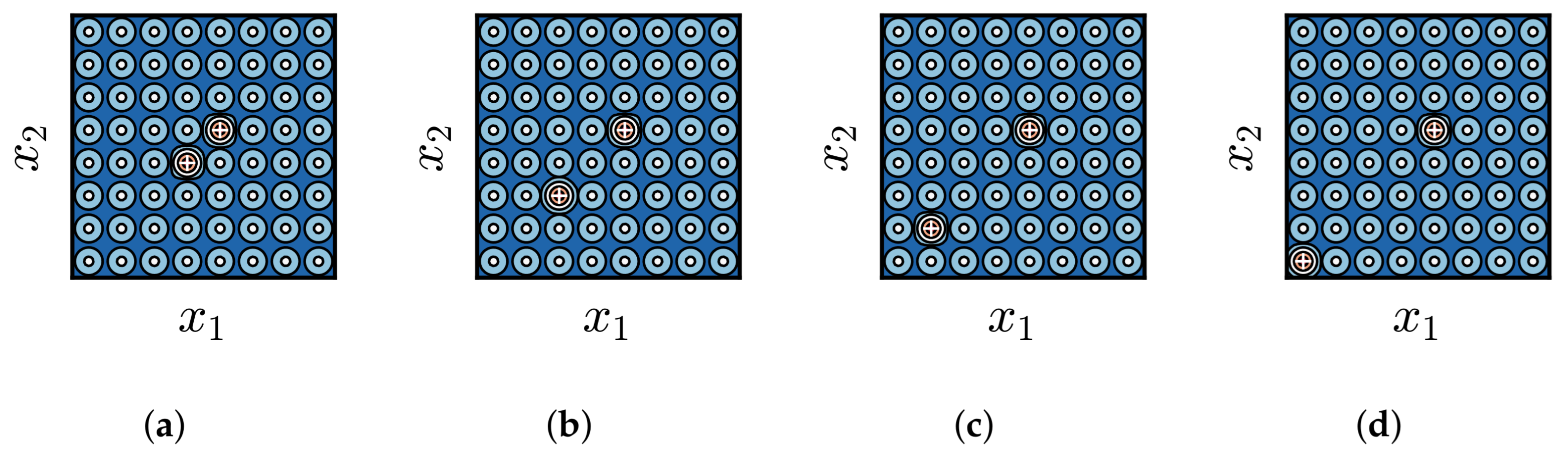
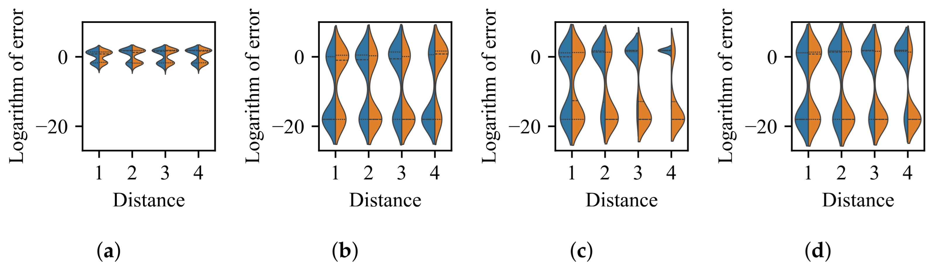
3.1. Impact of Difference in Size Between BoAs

The first benchmark scenario aims to highlight the effect of BoA size difference. It encompasses a series of problems, each featuring two global optima with peak functions, denoted as $s_1$, which ensure that the fitness distributions within each BoA are identical. Figure 2 depicts the fitness landscapes for four such problems with two decision variables, $x_1$ and $x_2$, while the size ratios of the BoAs associated with the two global optima are set to 1, 2, 4, and 8, respectively. The white crosses signify the locations of the global optima.

After 100 independent runs of each EC method with 20,000 evaluations on the four problems from the initial benchmark scenario, the logarithmic fitness errors obtained for each global optimum are presented in Figure 3. The figure presents violin plots for each EC method (in different subfigures) applied to problems with different BoA size ratios (represented on the x-axis). Each violin plot consists of two halves: the left, blue half illustrates the distributions of fitness errors for the first global optimum across the 100 runs, while the right orange half illustrates the distributions of fitness errors for the second global optimum across the same 100 runs. The fitness error for an optimum is defined as the objective distance between the optimum and the best solution found within its BoA. The distinct boundaries of the BoAs facilitate accurate differentiation of the fitness errors for different global optima.

The results indicate that when the BoA sizes for the two global optima are equal, each EC method has approximately a 50% likelihood of locating either global optimum, although the precision varies due to the inherent differences in the operators of the EC methods. As the disparity in BoA sizes grows, the probability of discovering the first global optimum decreases, while the chance of finding the second global optimum increases. This trend underscores that a greater difference in BoA size correlates with a more pronounced disparity in the attractiveness of the corresponding local optima.

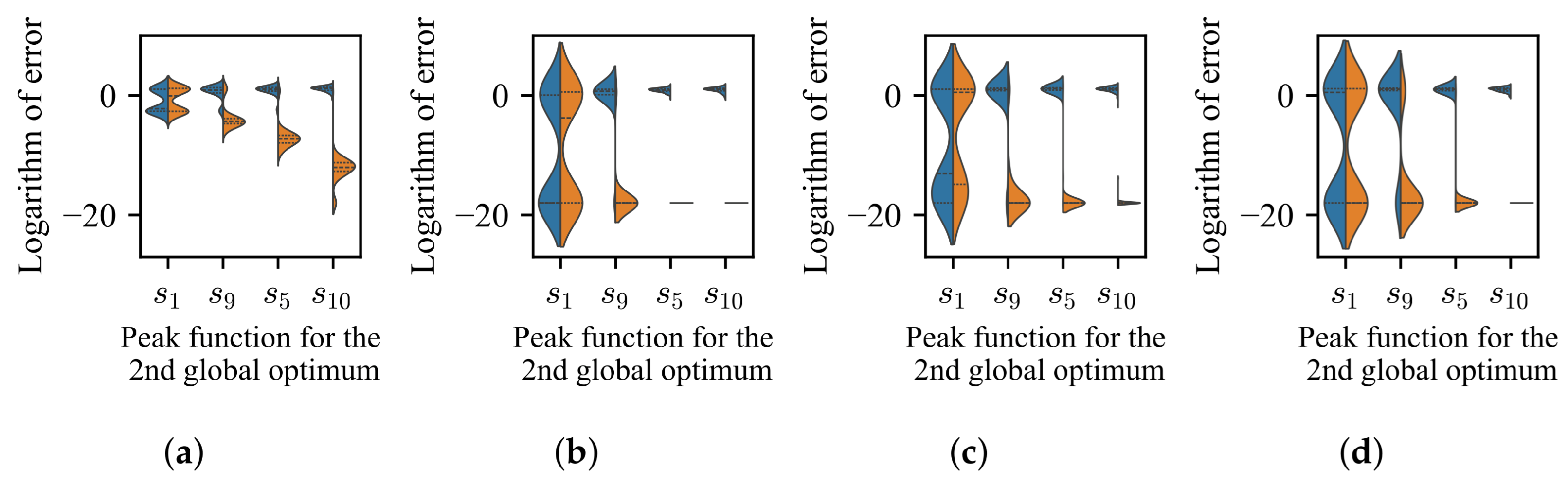
3.2. Impact of Difference in Average Fitness Between BoAs

In the second benchmark scenario, to demonstrate the impact of overall fitness differences between BoAs, each problem also features two global optima, with the BoA sizes for both being equal. Figure 4 illustrates the fitness landscapes for four such problems. To achieve this effect, the peak function for one global optimum was set to $s_1$, while the peak function for the other global optimum was varied across $s_1$, $s_9$, $s_5$, and $s_{10}$, respectively.

The two peak functions $s_1$ and $s_5$ were selected from the eight peak functions defined in the original paper [9]. Their expressions are as follows:

$$\begin{array}{cc}\hfill s_1(d,h)& =h-d^1{h}^0\hfill \end{array}$$

(1)

$$\begin{array}{cc}\hfill s_5(d,h)& =h-d^2{h}^{-1}\hfill \end{array}$$

(2)

where d represents the distance to the peak, and h represents the height of the peak. $s_5$ is designed to have a higher overall fitness than $s_1$.

To achieve the gradient variation in the overall fitness of the BoA of the second global optimum, we designed another two peak functions, $s_9$ and $s_{10}$. The peak function $s_9$ was designed to have an overall fitness between $s_1$ and $s_5$, while $s_{10}$ was designed to have a higher overall fitness than $s_5$. Their expressions are as follows:

$$\begin{array}{cc}\hfill s_9(d,h)& =h-d^{1.4}{h}^{-0.4}\hfill \end{array}$$

(3)

$$\begin{array}{cc}\hfill s_{10}(d,h)& =h-d^3{h}^{-2}\hfill \end{array}$$

(4)

Figure 5 presents the distribution of fitness values for 10,000 uniformly sampled solutions across the peak functions $s_1$, $s_9$, $s_5$, and $s_{10}$. A clear upward trend in overall fitness is observed as we progress from $s_1$ to $s_9$, then to $s_5$, and finally to $s_{10}$.

After 100 independent runs of each of the four EC methods with 20,000 evaluations on the four problems in the second benchmark scenario, the logarithmic fitness errors obtained for each global optimum are depicted in Figure 6. When the peak functions for the two global optima are identical, each EC method has approximately a 50% probability of locating either global optimum. As the difference in overall fitness between the BoAs of the two global optima increases, the likelihood of finding the first global optimum decreases, while the chance of locating the second global optimum rises. This suggests that a greater disparity in overall fitness between BoAs leads to a more pronounced difference in the attractiveness of the corresponding local optima.

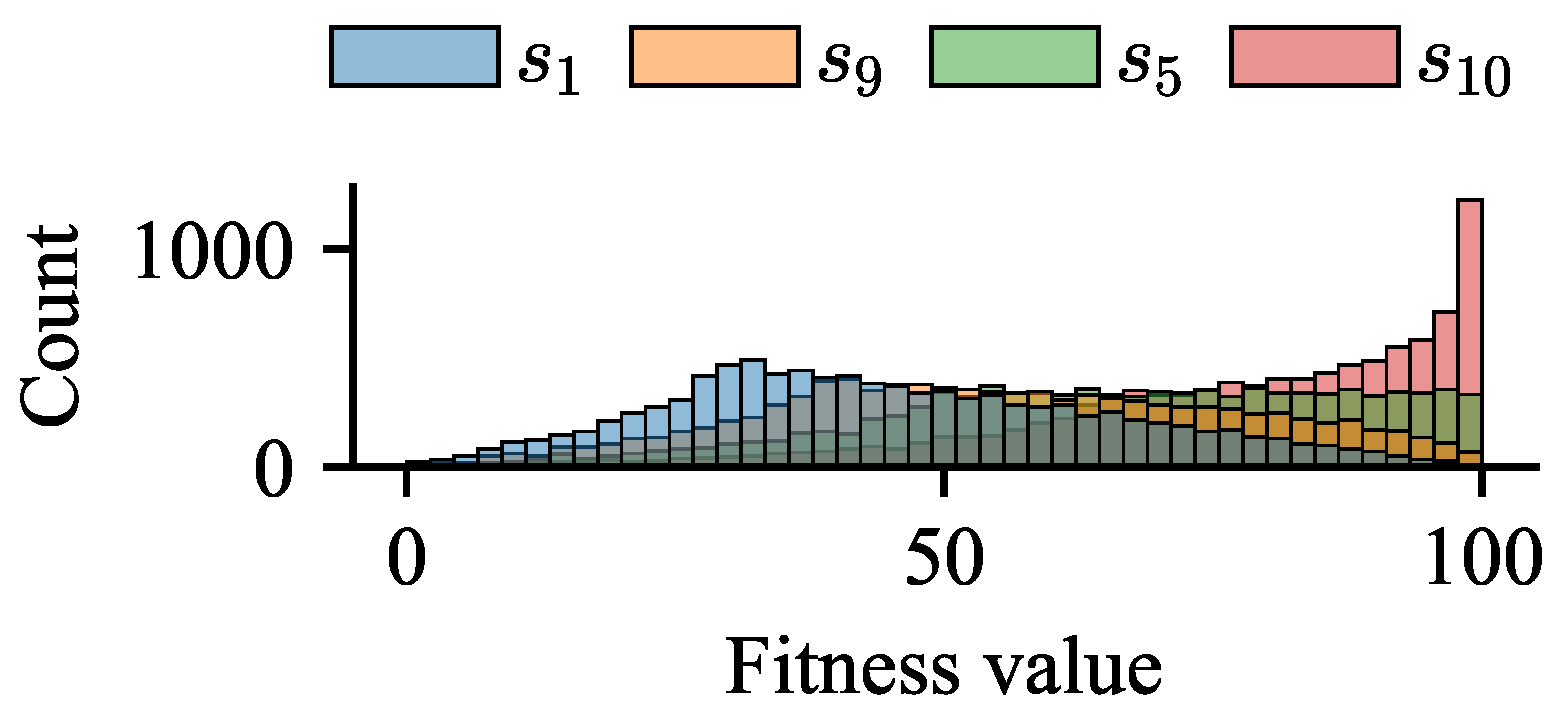
3.3. Impact of Difference in Distribution Between BoAs

In existing benchmark problems, global optima that are far from the center of the search space or adjacent to deceptive local optima are often challenging to locate. For example, in the test functions for the CEC 2005 special session on real-parameter optimization [39], the global optimum of F8, which has a narrow BoA, is located at the boundary of the search space. In F24 and F25, the global optima, also with narrow BoAs, are situated next to local optima with broad BoAs and high overall fitness values. To investigate whether the distribution of local optima significantly impacts the difference in attractiveness between them, we designed two additional benchmark scenarios.

The third benchmark scenario aims to verify whether a local optimum closer to the center of the search space is more attractive to the population. This scenario consists of four problems, each featuring 62 local optima and 2 global optima. The two global optima are positioned such that the distances between them are 1, 2, 3, and 4 times the distance between two nearest local optima, respectively, while the second global optimum remains near the center of the search space. The fitness landscapes for these problems are depicted in Figure 7. After 100 independent runs of the four typical EC methods with 20,000 evaluations, the logarithmic fitness errors obtained for each global optimum are shown in Figure 8.

The results indicate that for CMA-ES and SPSO-2011, the probability of locating the first global optimum decreases as it moves farther from the center of the search space. However, for SBX-GA, the probability of locating each global optimum remains relatively constant, regardless of the distance between the two global optima. For DE/rand/1, no clear relationship was observed between the probabilities of locating the two global optima and their distance.

A plausible explanation for these results is that the impact of the distance between a local optimum and the center of the search space on its attractiveness depends heavily on the specific operators of the EC method. For instance, CMA-ES, due to its Gaussian probability modeling, is more likely to generate offspring in areas closer to the center. Conversely, SBX-GA tends to generate offspring around each individual in the population, irrespective of the distribution differences among individuals. Therefore, the third scenario does not present a common challenge for all EC methods.

The final benchmark scenario is designed to verify whether a local optimum closer to a deceptive local optimum is less attractive to the population. In this scenario, each problem has 1 global optimum and 63 local optima. One of the local optima is made deceptive by setting its fitness slightly lower than that of the global optimum, and its peak function is $s_{10}$, while the peak function for the global optimum is $s_1$. The global optimum and the deceptive local optimum are positioned such that the distances between them in the four problems are 1, 3, 5, and 7 times the distance between two nearest local optima, respectively. Meanwhile, their distances to the center of the search space are always the same. The fitness landscapes for these problems are depicted in Figure 9, where the deceptive local optima are also indicated by white crosses.

After 100 independent runs of the four typical EC methods with 20,000 evaluations, the logarithmic fitness errors for the global optimum are presented in Figure 10. The results show no clear relationship between the distance from the global optimum to the deceptive local optimum and the probability of locating the global optimum for any of the four tested EC methods. Surprisingly, when the global optimum is far from the deceptive local optimum, the probability of finding the global optimum is lower than when it is adjacent to the deceptive local optimum.

3.4. Discussion

The performance of four representative EC methods has been evaluated across four benchmark scenarios, with the aim of investigating how several potentially critical factors influence the attractiveness differences between local optima. The experimental outcomes reveal no substantial correlation between the spatial distribution of local optima and their attractiveness. In other words, the impact of the difference in distribution between BoAs depends heavily on the reproduction operators adopted by the EC method.

On the other hand, for all the four tested EC methods, the differences in size and average fitness between BoAs significantly affect the relative attractiveness of the corresponding local optima. If we keep one of these two differences constant, the other difference can be equivalently attributed to the difference in the size of the superior region (e.g., the area where the fitness value is above the average). This makes it easier to understand the essence of the differences in attractiveness among various local optima to the population: as long as the BoA of a local optimum contains a larger superior region, then for any objective-driven EC method, the individuals within it are inherently more likely to be retained during the process of survivor selection.

Since between BoAs, the differences in size and average fitness are merely different manifestations of the difference in size of the superior region, we can choose to focus on just one of them. Considering that the difference in size is easier to control than the difference in average fitness, we only used the benchmark scenario detailed in Section 3.1 in our subsequent tests of niching methods.

It is worth noting that the dimensions of problems in the benchmark scenario are all set to 2. The reason for not using higher-dimensional problems is that in Free Peaks, increasing the difference in attractiveness between local optima does not require raising the problem dimension. Moreover, a problem dimension of 2 can actually improve experimental efficiency, making it easier to identify the performance limits of some EC methods with high time complexity.

4. Niching Techniques

In niching methods, it is common to see a combination of various niching techniques. The difference between these niching techniques primarily lies in the way in which they define the neighborhood for restricted competition. According to this factor, existing niching techniques can be grouped into five categories. Their descriptions are as follows.

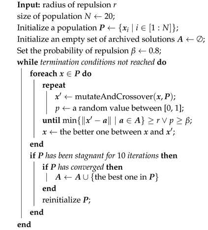
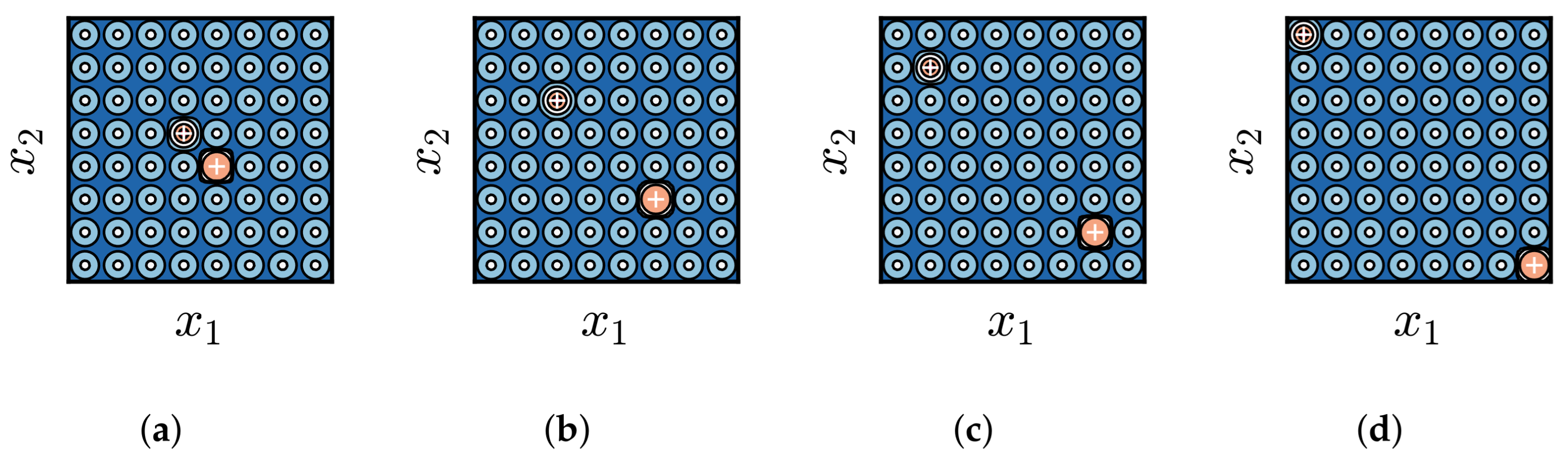
• Radial repulsion: If an individual is deemed to be sufficiently close to a local optimum, then all other individuals that are at a distance greater than a given threshold from this individual cannot be replaced by this individual or any other individuals that are at a distance less than the given threshold from this individual.
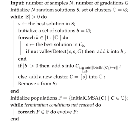
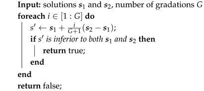
• Valley detection: An individual cannot be replaced by another individual if there exists a worse individual between them. The method to determine whether such a worse individual exists involves sampling and evaluating a specified number of gradation points at equal intervals along the line segment connecting the two individuals.
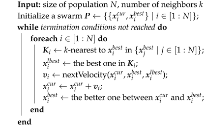
• k-nearest neighbors: An individual can only be replaced by a given number of individuals that are closest to it.
• Clustering with a specified number of groups: Individuals are divided into a specified number of equally sized groups, with the aim of ensuring that the centers of these groups are as optimal and as far apart from one another as possible. Competition is confined within each group.
• Clustering with an adaptive number of groups: Individuals are divided into a dynamically adjusted number of groups based on their density in the search space or dominance relationships. Competition is confined within each group.

Some representative niching methods that employ these techniques are listed in

Table 1. Niching techniques adopted by niching methods.

Niching Method	Niching Technique
	Radial Repulsion	Valley Detection	$\mathit{k}$-Nearest Neighbors	Clustering with a Specified # of Groups	Clustering with an Adaptive # of Groups
Sharing [10]	✓
Clearing [11]	✓
Forking-GA [12]	✓
Speciation [13]	✓
PMODE [14]	✓
RS-CMSA [7]	✓	✓
Multinationl EA [15]		✓
DNC-RM [16]		✓
TSC2 [17]		✓
HillVallEA [18]		✓
CDE [19]			✓
DE/nrand/1 [20]			✓
Ring-PSO [21]			✓
LIPS [22]			✓
NCDE [23]			✓
NSDE [23]				✓
Self-CCDE [24]			✓	✓
Self-CSDE [24]			✓	✓
DHNDE [25]				✓
NEA2 [26]					✓
HTS-CDE [27]			✓		✓
AMP-DE [28]					✓
EMO-MMO [29]					✓
ANDE [30]			✓		✓
NCD-DE [31]			✓		✓
ESPDE [32]			✓		✓
HGHE-DE [33]					✓

. From this table, three intriguing observations can be made:

• Techniques that appeared decades ago, namely radial repulsion and valley detection, are still adopted in some state-of-the-art niching methods;
• In the niching methods of the past decade, the k-nearest neighbors technique and two clustering-based techniques have gained significant popularity;
• The k-nearest neighbors technique is frequently used in conjunction with other techniques.

Combining the first two points inevitably raises the following question: which have more development potential—older technologies or newer ones? The last point also makes one curious: which technique actually plays a more critical role?

Fortunately, it is not difficult to identify the key parameters that determine the effectiveness of each technique. For radial repulsion, the critical parameter is the threshold distance, commonly referred to as the niche radius. For valley detection, the two key parameters are the population size and the number of gradation points. For k-nearest neighbors, the two key parameters are the population size and the number of neighbors. In the case of clustering with a specified number of groups, the two key parameters are the population size and the group size. Finally, for clustering with an adaptive number of groups, the common key parameter is the population size.

The subsequent subsections describe how the experiments were conducted in groups, with each group corresponding to a specific niching technique, to validate the aforementioned reasoning for key parameters while exploring the developmental potential of different niching techniques.

4.1. Radial Repulsion

To illustrate the influence of the threshold distance in radial repulsion on reducing the disparity in attractiveness between optima, we have developed a DE method that incorporates a mechanism to restart the search process upon population convergence, while avoiding previously discovered optima. This method, referred to as local repulsion DE (LRDE), is detailed in Algorithm 1. The sole parameter of LRDE is the repulsion radius r, which corresponds to the threshold distance in radial repulsion. An archive $\mathit{A}$ is maintained, containing the best solutions from the converged population. During the trial vector generation, if a trial vector’s distance to any solution in $\mathit{A}$ is less than r, it is discarded and a new one is generated.

Algorithm 1: LRDE$\left(r\right)$

To demonstrate the impact of the repulsion radius r, we conducted tests using LRDE with r varying from 0.05 to 0.95 in the benchmark scenario outlined in Section 3.1. The logarithmic fitness errors for the first, more challenging global optimum are depicted in Figure 11. In the heatmap, the colors in the grid represent the average fitness error over 100 independent runs on a problem with a given size ratio of the two global optima’s BoAs when r is set to a given value.

The results indicate that when the BoAs of the two global optima are of equal size, any value of r can successfully lead to the location of the first global optimum. When the difference in size between the two BoAs varies, there still exists a range of r values that ensures the highest precision for locating the first global optimum, indicating that both global optima can be effectively located. This raises the following question: how do existing EC methods with radial repulsion set the value of the threshold distance? Does the relationship between the value of the threshold distance and the performance of LRDE also apply to these EC methods?

To address this question, we selected two state-of-the-art methods from those listed in Table 1 that use radial repulsion: covariance matrix self-adaptation ES (CMSA-ES) with repelling subpopulations (RS-CMSA) [7], and penalty-based DE for multimodal optimization (PMODE) [14]. Similarly to LRDE, these methods also reinitialize the population upon convergence. However, unlike LRDE, they dynamically adjust their threshold distances for radial repulsion at each restart—referred to as the penalty radius in PMODE and the taboo distance in RS-CMSA. To this end, we recorded all the values to which the threshold distances were adjusted during the execution of these two EC methods in the two benchmark scenarios, with the maximum number of evaluations set to 20,000. The distribution of these values is presented in Figure 12.

When comparing these distributions with the results illustrated in Figure 11, it is evident that both RS-CMSA and PMODE have adjusted their threshold distances for radial repulsion to values suitable for LDRE. So will these two EC methods exhibit similarly good performance, as expected? Figure 13 provides the answer, showing the distribution of fitness errors for these two EC methods for the two global optima in the benchmark scenarios. The results indicate that both methods are capable of locating the global optima, regardless of the disparities in size between the BoAs.

However, as the difference in size between BoAs further increases, the appropriate range for the distance threshold narrows. This trend is clearly illustrated in Figure 11, highlighting the challenge. To further investigate this, we increased the size ratio of the two global optima’s BoAs to a range from 10 to 100, and recorded the fitness errors of LRDE for the first global optimum, with various values of r, on these problems. As shown in Figure 14, the trend of the narrowing appropriate range for the distance threshold continues as the size difference between BoAs increases. When the size ratio of the two global optima’s BoAs reaches 100, even the optimal value of $r=0.35$, among the sampled values, does not achieve the highest average precision for locating the first global optimum.

Since a sufficiently precise threshold distance cannot be found through simple equidistant sampling, can it be obtained through the dynamic adjustment mechanisms in RS-CMSA or PMODE? To address this question, we selected four problems with the size ratio of the BoAs of the two global optima set to 10, 40, 70, and 100, respectively, and recorded all the values to which the threshold distances were adjusted during the execution of these two EC methods on these four problems, with the maximum number of evaluations set to 20,000. The distribution of these values is presented in Figure 15.

Unfortunately, the distributions in Figure 15 do not appear to differ significantly from those in Figure 12. Therefore, it is not surprising to observe, from the distributions of the fitness errors of these two methods for the two global optima, as shown in Figure 16, that both methods have a lower chance of locating the first global optimum as the size ratio of the BoAs increases. Specifically, when compared to PMODE, the threshold distances of RS-CMSA correspond to much larger average fitness errors, as indicated by the heatmap in Figure 14. Consequently, the probability of RS-CMSA locating the first global optimum is lower than that for PMODE.

Valley Detection

According to the experiments in the previous subsection, the potential for adjusting the threshold distance in radial repulsion appears to be limited. Even though there exists a range of values that can help locate the desired optima with tiny sizes or low overall fitness, an established method for determining this range is not available. However, this is not the case for valley detection. If computational cost is not a concern, a challenging optimum can always be found by increasing the population size or the number of gradations.

To validate this point, we introduced a two-stage EC method, referred to as hill–valley ES (HVES). This approach is a simplified variant of the hill–valley evolutionary algorithm (HillVallEA) [18]. The pseudocode for HVES is provided in Algorithm 2. During the first stage, a set of random solutions is generated and then grouped into clusters. This clustering ensures that there are no valleys between any two solutions within the same cluster, while a valley is guaranteed to exist between solutions from different clusters, as determined by the valley detection method detailed in Algorithm 3. In the second stage, CMSA-ES [40] is applied to each cluster, using the initial distribution calculated by solutions within the cluster. The specific procedure for initializing CMSA-ES with a given group of solutions is consistent with the process in HillVallEA.

HVES has two parameters: the number of samples, denoted as N, which corresponds to the population size in valley detection; and the number of gradations, denoted as G. We evaluated HVES with varying values of N and G on the problem where the size ratio of the BoAs for the two global optima was set to 8. The results are illustrated in Figure 17a. In the heatmap, the color of each cell represents the average fitness error the first global optimum, with specific values of N and G applied to HVES over 100 runs. A clear trend emerges from the data, indicating that an increase in either the number of samples or gradations enhances the likelihood of locating the first global optimum.

To delve deeper into the impact of these two parameters on the performance of HVES, we conducted further experiments by fixing one parameter and adjusting the other, observing how changes in the variable parameter could mitigate the challenge posed by the increasing difference in BoA sizes. The outcomes of varying N or G are depicted in Figure 17b and c, respectively, with G fixed at 2 in the former case and N at 50 in the latter. The results suggest that, when confronted with a linear increase in the size ratio of BoAs, achieving a similar effect through the adjustment of G requires a linear growth, whereas a comparable outcome via changes in N necessitates an exponential increase.

Algorithm 2: HVES$(N, G)$

Algorithm 3: valley Detect$({\mathit{s}}_1, {\mathit{s}}_2, G)$

Although the effects of the population size and the number of gradations in valley detection are evident in the case of HVES, their generalizability remains to be confirmed across other instances. To address this, we selected two relatively recent EC methods that incorporate valley detection: improved topological species conservation (TSC2) [17] and HillVallEA. We evaluated TSC2, HillVallEA, and HVES using the benchmark scenario outlined in Section 3.1, with a maximum of 20,000 evaluations. For TSC2 and HVES, the population size (or number of samples in the case of HVES) was set to 20, and the number of gradations was fixed at 2. As for HillVallEA, it is parameter-free. The results are presented in Figure 18.

According to the results, for TSC2 and HVES, the probability of locating the first global optimum decreases as the disparity in size between BoAs increases. Regarding HillVallEA, the situation is quite distinct. Regardless of the variation in the size difference between the BoAs of the two global optima, HillVallEA consistently locates the first global optimum. The underlying reason is that, as previously stated, HillVallEA is parameter-free; therefore, the population size used for valley detection—referred to as the number of samples in HillVallEA—and the number of gradations are dynamically adjusted. There is, however, a distinction between these parameters. While the number of gradations for identifying the valley between two solutions is dependent on their distance, the numbers of gradations are designed to focus around two. Concerning the number of samples, it is worth noting that, similarly to LRDE, RS-CMSA, and PMODE, HillVallEA also reinitializes the population following convergence, with the number of samples doubling each time prior to reinitialization. Consequently, if we record the distribution of values used as the number of samples, as depicted in Figure 19, the maximum value attained is $2^{11}$. When this aspect is considered alongside the average fitness error of HVES for the first global optimum, as shown in Figure 17, the performance of HillVallEA becomes less surprising.

4.2. k-Nearest Neighbors

The k-nearest neighbors technique has remained popular since its inception, particularly within DE and PSO methods. This popularity stems from the fact that in DE and PSO, survivor selection occurs individually, either between an individual and its trial vector or between a particle and its pbest. Consequently, the k-nearest neighbors technique can be seamlessly implemented by choosing the base vector for an individual in DE, or the lbest for a particle in PSO, from among its k-nearest neighbors.

To evaluate the impact of the k-nearest neighbors technique, we chose five representative DE and PSO methods: crowding DE (CDE) [19], DE/nrand/1 [20], neighborhood-based CDE (NCDE) [23], PSO with ring topology [21], and distance-based locally informed PSO (LIPS) [22]. We did not include some more recent methods as they incorporate additional niching techniques.

As previously noted, it is necessary to examine the influence of two parameters associated with the k-nearest neighbors technique: the number of neighbors k and the population size N. Among the selected EC methods, the three DE methods maintain a fixed k value of 2, while the PSO with ring topology is limited to four configurations, R2PSO, R3PSO, R2PSO-LHC, and R3PSO-LHC, where k can only be 2 or 3. LIPS, on the other hand, dynamically adjusts k between 2 and 5. To address this limitation, we propose a novel PSO method, k-nearest PSO (kNPSO), which allows for a freely adjustable k value. The detailed pseudocode for kNPSO is provided in Algorithm 4. The only distinction between kNPSO and traditional PSO methods is that a particle’s lbest is determined from its k-nearest neighbors.    

Algorithm 4: kNPSO$(N, k)$

To illustrate the effect of k and N on the performance of kNPSO, we conducted a test on the problem featuring two global optima with identical peak functions, but with a BoA size ratio of 8. The average fitness error for the first global optimum is depicted in Figure 20a. Each cell’s color in the heatmap represents the fitness error of kNPSO with specific k and N values.

The findings reveal a clear trend: a larger population or a smaller number of neighbors generally leads to a lower average fitness error for the first global optimum, suggesting a higher likelihood of locating the optimum. Nevertheless, the number of neighbors cannot be arbitrarily reduced. If $k=2$ does not suffice to find a challenging optimum, increasing the population size is the only recourse. Fortunately, as shown in Figure 20b, which displays the average fitness error for the global optimum with $k=2$ and N varying from 10 to 50 across problems with BoA size ratios from 10 to 50, a linear increase in population size can offset the difficulty posed by a linearly growing BoA size ratio.

It is important to note that the performance of kNPSO may not be indicative of all EC methods utilizing the k-nearest neighbors technique. Therefore, we tested kNPSO and the five aforementioned DE and PSO methods in the benchmark scenario described in Section 3.1. For each method, we set the population size to 20 and the maximum number of evaluations to 20,000. In kNPSO, the number of neighbors was set to two, and R2PSO was chosen to represent PSO with ring topology. The remaining parameters were set according to the recommendations in the original papers. The results are presented in Figure 21.

The results indicate that all the other five DE and PSO methods employing the k-nearest neighbors technique exhibit behavior similar to that of kNPSO: an increase in the difference in size between the BoAs of the two global optima tends to raise the average fitness error for the first global optimum.

4.3. Clustering with a Specified Number of Groups

In Table 1, some readers may find it intriguing that NCDE and neighborhood-based species-based DE (NSDE), which were introduced in the same paper, are categorized under two different techniques for restricted competition. In contrast, self-CCDE and self-CSDE, which are cluster-based CDE and SDE (species-based DE) with a self-adaptive strategy, and are also proposed in the same paper, are grouped within the same technique category for restricted competition.

Before explaining our above categorization, it is essential to distinguish between the following two techniques: k-nearest neighbors and clustering with a specified number of groups. If a set of random individuals is partitioned using the clustering with a specified number of groups method, two closely located solutions might end up in separate groups, precluding them from competing with one another. However, if the k-nearest neighbors approach is used, these solutions would be able to compete.

So if we delve into the details of NCDE, NSDE, self-CCDE, and self-CSDE, it becomes clear that the latter three select an individual’s base vector from its affiliated group, whereas NCDE chooses the base vector from among the individual’s neighbors. Thus, NCDE utilizes the k-nearest neighbors technique, while NSDE, self-CCDE, and self-CSDE employ the clustering with a specified number of groups technique.

After evaluating four EC methods that use the clustering with a specified number of groups technique—NSDE, self-CCDE, self-CSDE, and dynamically hybrid niching DE (DHNDE) [25]—in the benchmark scenario described in Section 3.1, with a population size of 20, a group size of 5 (resulting in 4 groups), and a maximum of 20,000 evaluations, we observed some performance differences. The outcomes are depicted in Figure 22.

The results indicate that the performances of NSDE, self-CCDE, and self-CSDE are akin to those of EC methods using the k-nearest neighbors technique. Generally, as the size ratio of the BoAs of the two global optima increases, the average fitness error for the first global optimum rises.

Regarding DHNDE, it performs markedly better than the other three methods when the BoA size ratio is large. This can be attributed to the fact that the effective population size in DHNDE, after including an inferior archive, is actually triple the input population size, unlike in NSDE, self-CCDE, or self-CSDE. After setting the population size to 7, as demonstrated in Figure 23, the performance of DHNDE becomes much more similar to that of the other three EC methods.

Having elucidated the reasons behind the performance differences, it is logical to select NSDE for testing the impact of the parameters of the clustering with a specified number of groups technique, namely group size and population size. We assessed NSDE with various population and group sizes on the problem where the BoA size ratio is 8. The findings, illustrated in Figure 24a, suggest that a larger population or smaller group tends to reduce the average fitness error, thereby enhancing the chances of finding the optimal solution. An anomaly occurs at a population size of 25 and a group size of 20, possibly because the resulting group size ratio approximates the BoA size ratio.

Given that the difficulty of locating the first global optimum escalates with the BoA size ratio, how effective is the clustering with a specified number of groups technique in addressing this challenge through parameter adjustment? Since the group size cannot be reduced below five due to the requirement for selecting parent vectors in DE, increasing the population size remains the only viable option for amplifying the technique’s effectiveness. Similarly to in the k-nearest neighbors technique, a linear increase in the population size can mitigate the challenges posed by a linear growth in the BoA size ratio. This is illustrated in Figure 24b, which depicts the average fitness error for the global optimum when the group size is set to 5, and the population size varies from 25 to 125, across problems with BoA size ratios ranging from 10 to 50.

4.4. Clustering with an Adaptive Number of Groups

For any of the four aforementioned categories of niching techniques, the commonalities among the niching methods adopting such a technique can more or less be discerned from their nomenclature and the citation relationships within the literature. However, for this last technique under discussion, it is difficult to identify a unifying characteristic among the niching methods that use it, except for the fact that each method adopts a parameter-free clustering approach and the upper limits of their effects are constrained by the population size.

Before substantiating the aforementioned point, we shall first examine their performances in the benchmark scenario described in Section 3.1. The niching methods involved in this experiment included the niching CMA-ES with nearest-better clustering (NEA2) [26], history-based topological speciation CDE (HTS-CDE) [27], evolutionary multiobjective optimization-based multimodal optimization (EMO-MMO) [29], automatic niching differential evolution (ANDE) [30], DE based on niche center distinguish (NCD-DE) [31], and ESPDE [32].

For each niching method, the population size was set to 20, and the maximum number of evaluations was set to 20,000. It is noteworthy that only NEA2 incorporates a mechanism for restarting after population convergence, which means its fitness error for a run actually represents the best value out of multiple runs. To ensure comparability, the version of NEA2 without restart was utilized in this experiment. The results are presented in Figure 25.

The results reveal limited commonalities in performance across these niching methods. Generally, an increase in the size ratio of BoAs significantly reduces the average fitness error for the first global optimum for each of the six methods.

The differences in performance are much more pronounced. Compared to the other four methods, HTS-CDE and EMO-MMO exhibit notably poorer overall performance. Even when the sizes of the BoAs for the two global optima are identical, the average fitness error of HTS-CDE remains high. EMO-MMO’s performance is almost on par with that of EC methods lacking niching techniques.

To delve deeper into the underlying reasons for the observed disparities, we recorded the group centers obtained by each method in the above benchmark scenario, and illustrate the distributions of the numbers of group centers in the BoAs of each global optimum in Figure 26. Each violin plot shows the distribution of the numbers of group centers in the two BoAs, with the left, blue section representing the BoA of the first global optimum and the right, orange section representing that for the second. For HTS-CDE, the seed solutions serve directly as the group centers. For the other methods, the best solution in each group is identified and treated as the group center.

The results elucidate most of the observed disparities. For EMO-MMO, the number of group centers in the BoA of the first global optimum decreases to nearly zero as the size ratio of the BoAs increases to 8. Clearly, the absence of a group center in its BoA hinders the location of the first global optimum.

An anomaly is the performance of HTS-CDE. The results indicate that HTS-CDE consistently achieves the ideal group centers in the benchmark scenario. Other methods tend to obtain more than one group center in each BoA, particularly in the BoA of the second global optimum, leading to redundant searches. Unlike those methods, HTS-CDE secures exactly one group in each BoA. This outcome justifies its computational time, which far exceeds that of other methods. But why does HTS-CDE fail to locate both global optima, given the presence of a seed solution in each BoA? Upon visualizing the evolutionary process, we found that the inefficiency of the local search operators employed by HTS-CDE is to blame. Despite the proximity of the seed solution in the BoA of the first global optimum to the actual optimum, no additional offspring are generated around the seed, causing stagnation in the improvement of the seed solution.

Having observed the common challenge faced by EC methods employing the clustering with an adaptive number of groups technique in locating the first global optimum as the size ratio of BoAs increases, it is essential to determine whether a larger population can alleviate this difficulty. Thus, we tested these methods on a problem where the size ratio of the BoAs for the two global optima was set to 20, observing the fitness errors of these methods at different population sizes. The results, displayed in Figure 27, show that for each method, the average fitness error for the first global optimum decreases as the population size grows, suggesting that a larger population can aid in finding the more challenging optimum.

5. Conclusions

Since in most existing benchmark problems, the underlying reasons for differential attractiveness of local optima to populations are often coupled and the boundaries of BoAs are often indistinct, conducting quantitative analyses of the effectiveness of various niching methods is difficult.

To address this issue, the present study took continuous optimization as a starting point, and utilized Free Peaks [9] to simulate benchmark scenarios with controllable difficulty in the face of a multimodal problem. Through experiments involving a wide array of representative niching methods, the potential of underlying niching techniques is thoroughly examined.

From our empirical studies, we have drawn the following conclusions:

• The difference in size of the superior region between BoAs represents a common obstacle for most EC methods, whereas the differential distribution of local optima primarily hinders EC methods with less uniform reproduction operators, such as CMA-ES.
• After classifying the niching techniques into five categories, each characterized by a unique set of key parameters, the potential of each category obtained through parameter tuning is as follows:

  –

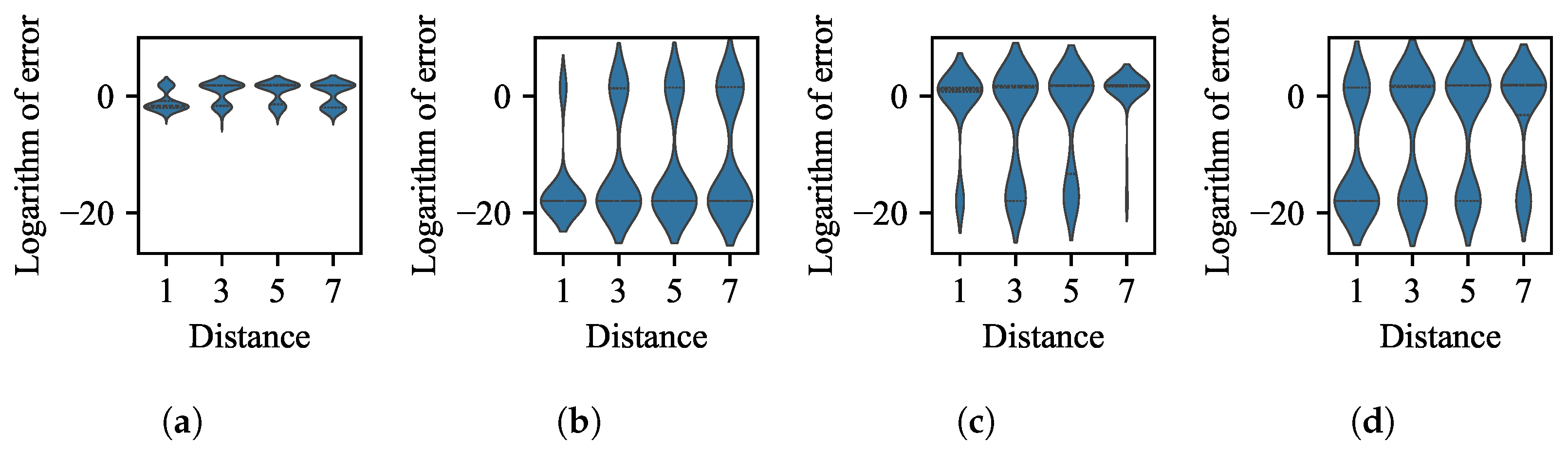
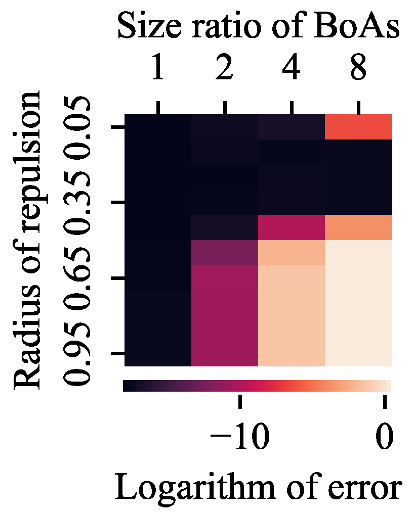
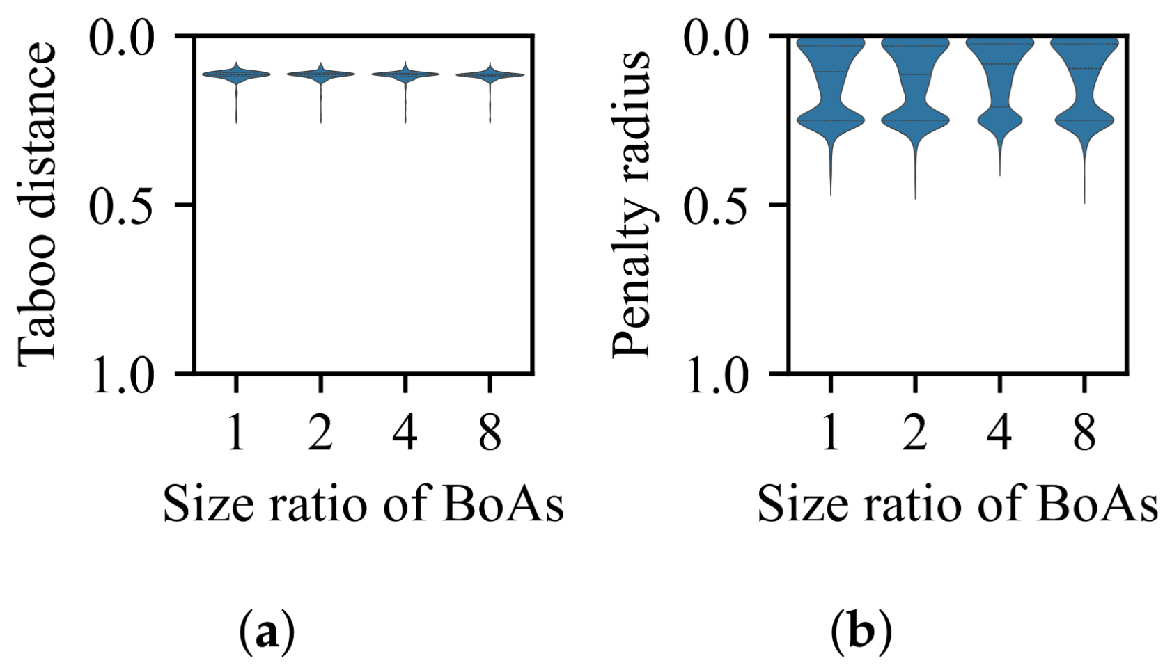
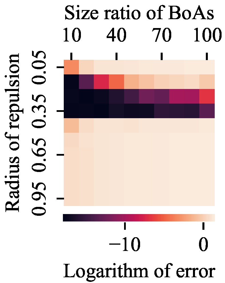
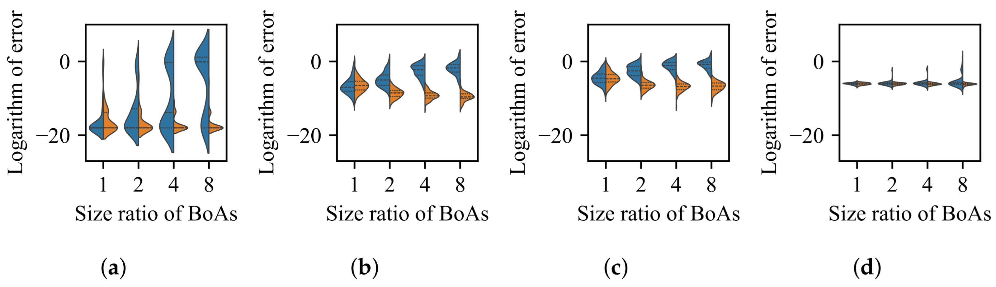
  The radial repulsion technique can be enhanced by setting the repulsion radius within a narrower and more suitable range; however, determining the optimal range remains challenging.

  –

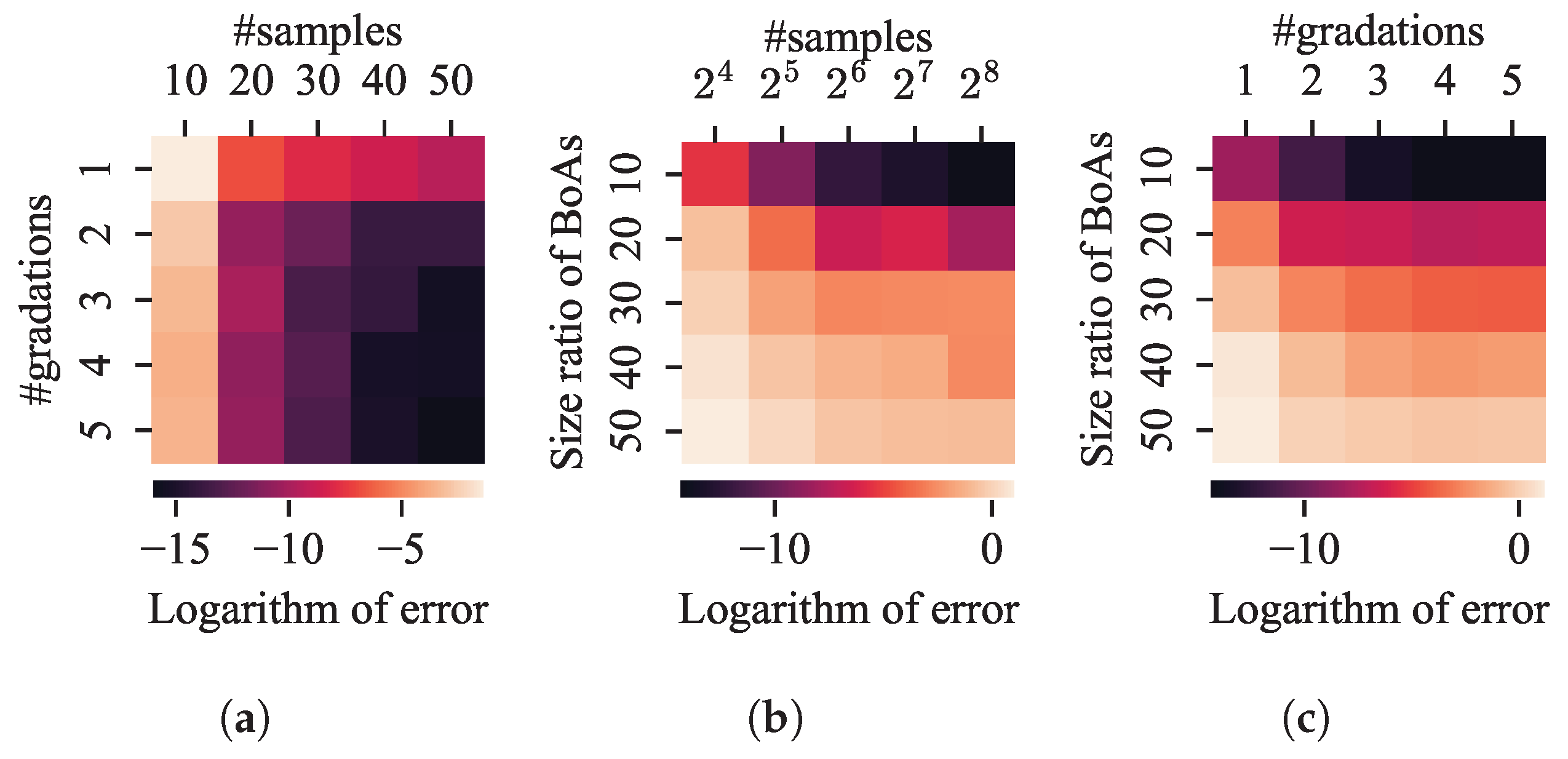
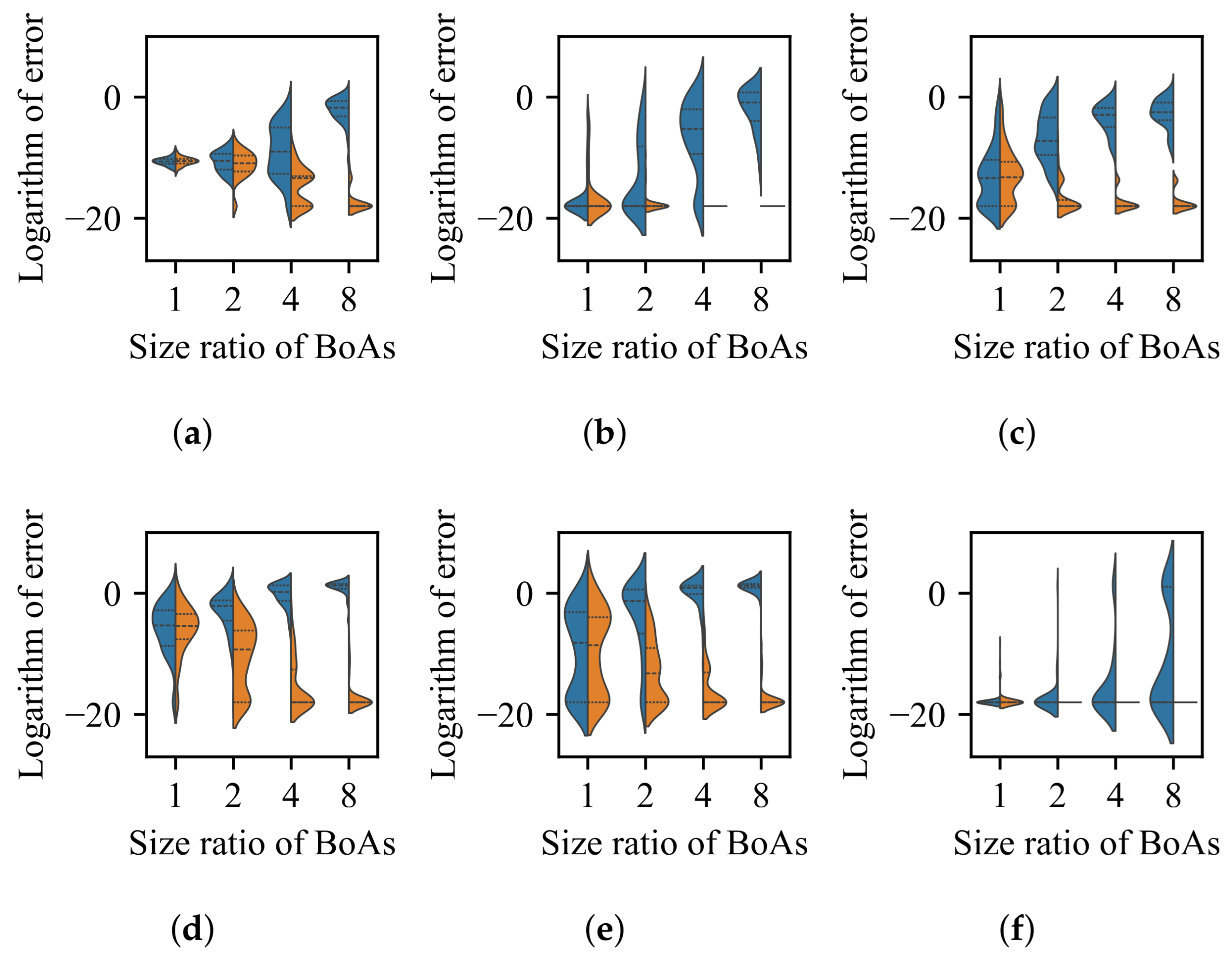
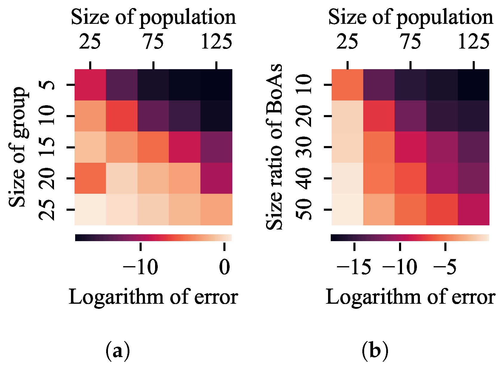
  The performance of the valley detection can be improved by increasing the population size or the number of gradations. Nevertheless, an exponential increase in population size is necessary to counteract the challenge posed by a linear increase in the difference between BoA sizes.

  –

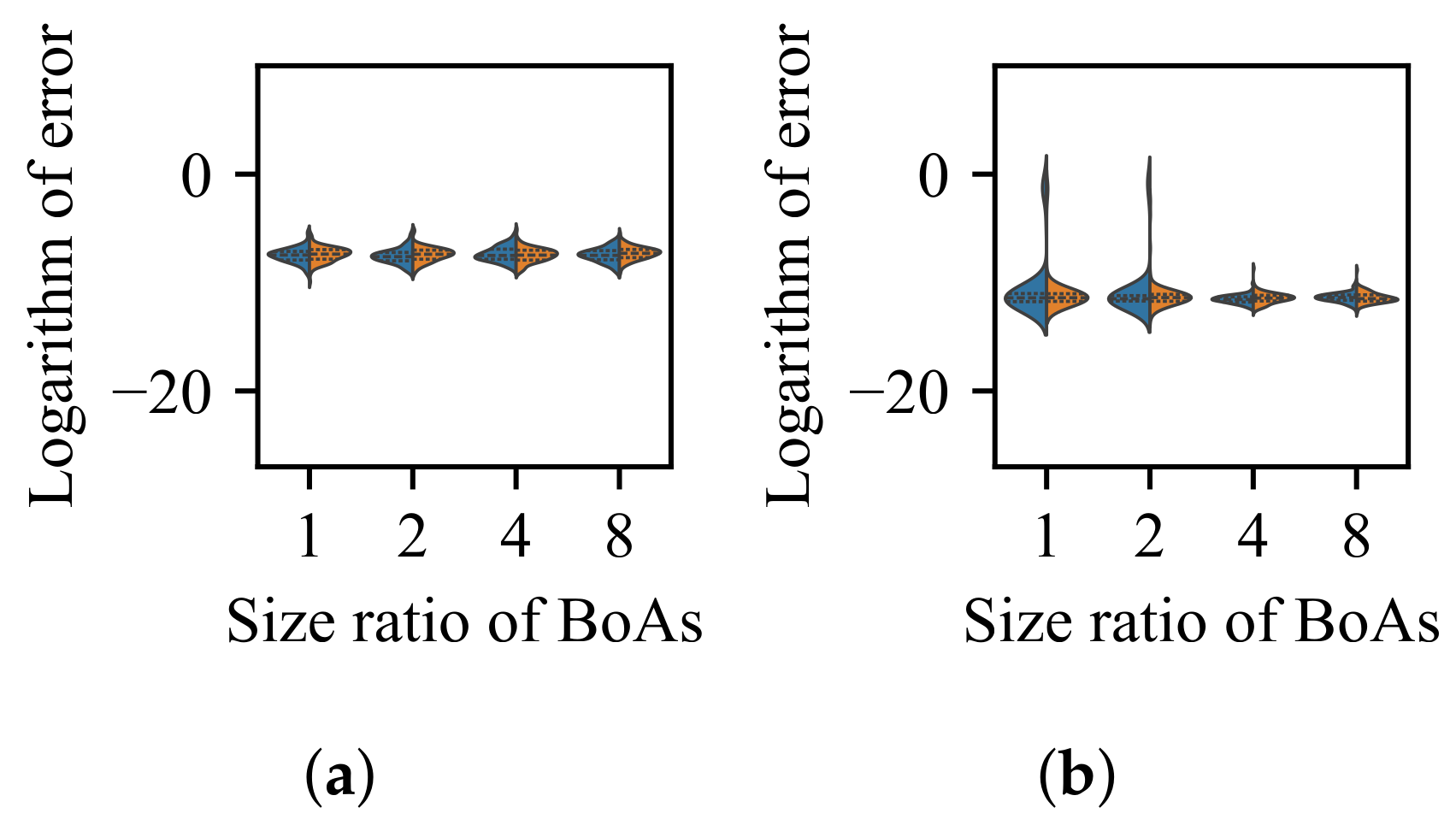
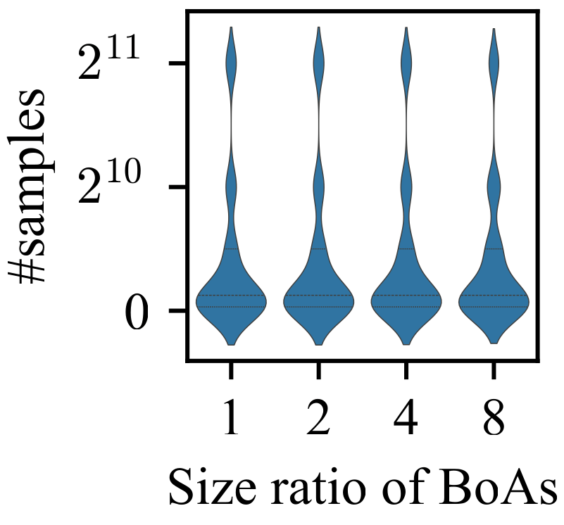
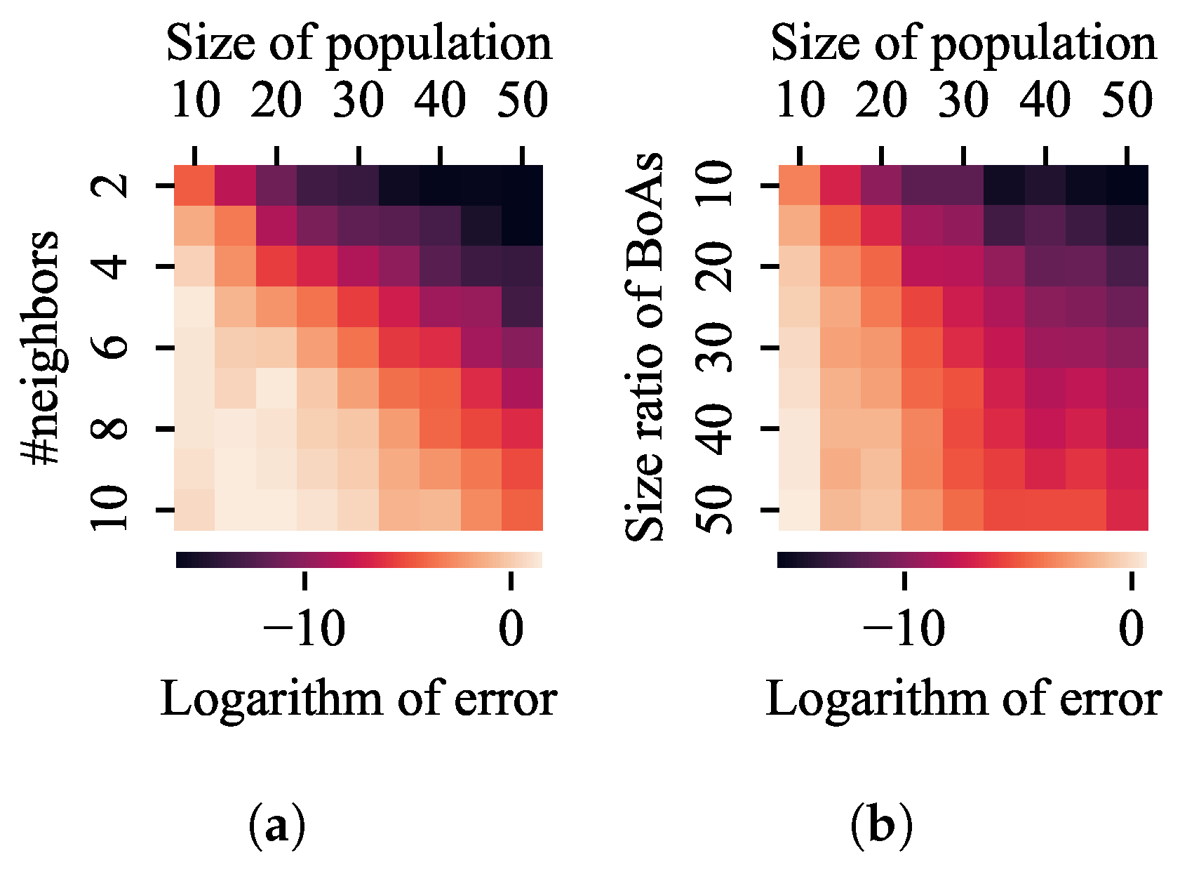
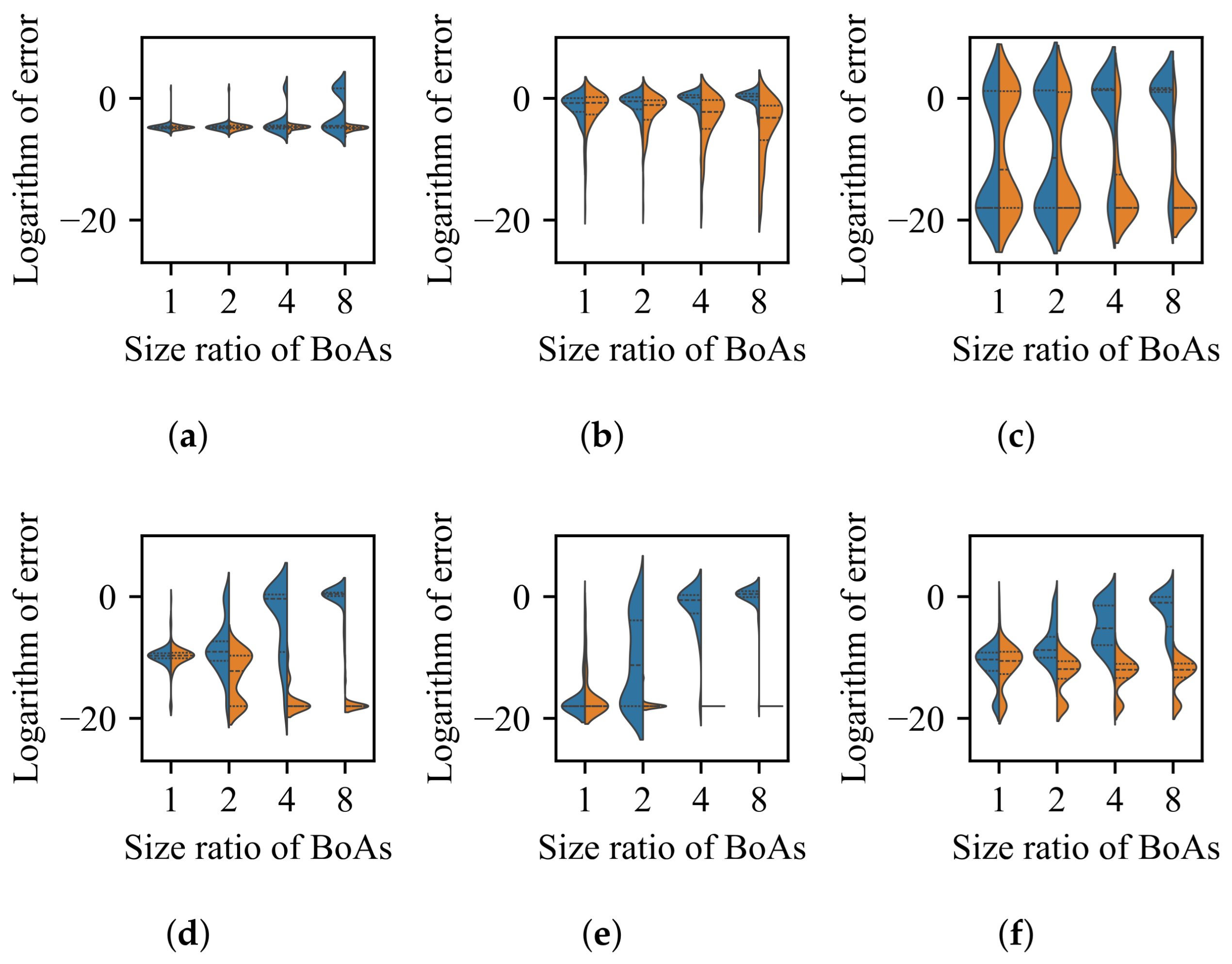
  Both the k-nearest neighbors and clustering with a specified number of groups techniques can be improved by reducing the number of neighbors or the group size while increasing the population size. Despite a minimum threshold for the number of neighbors or group size, a linear increase in population size can overcome the challenge presented by a linear growth in the difference between BoA sizes.

  –

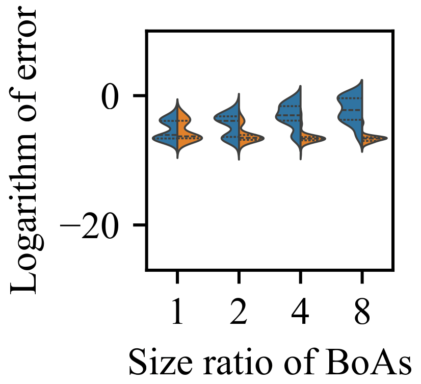
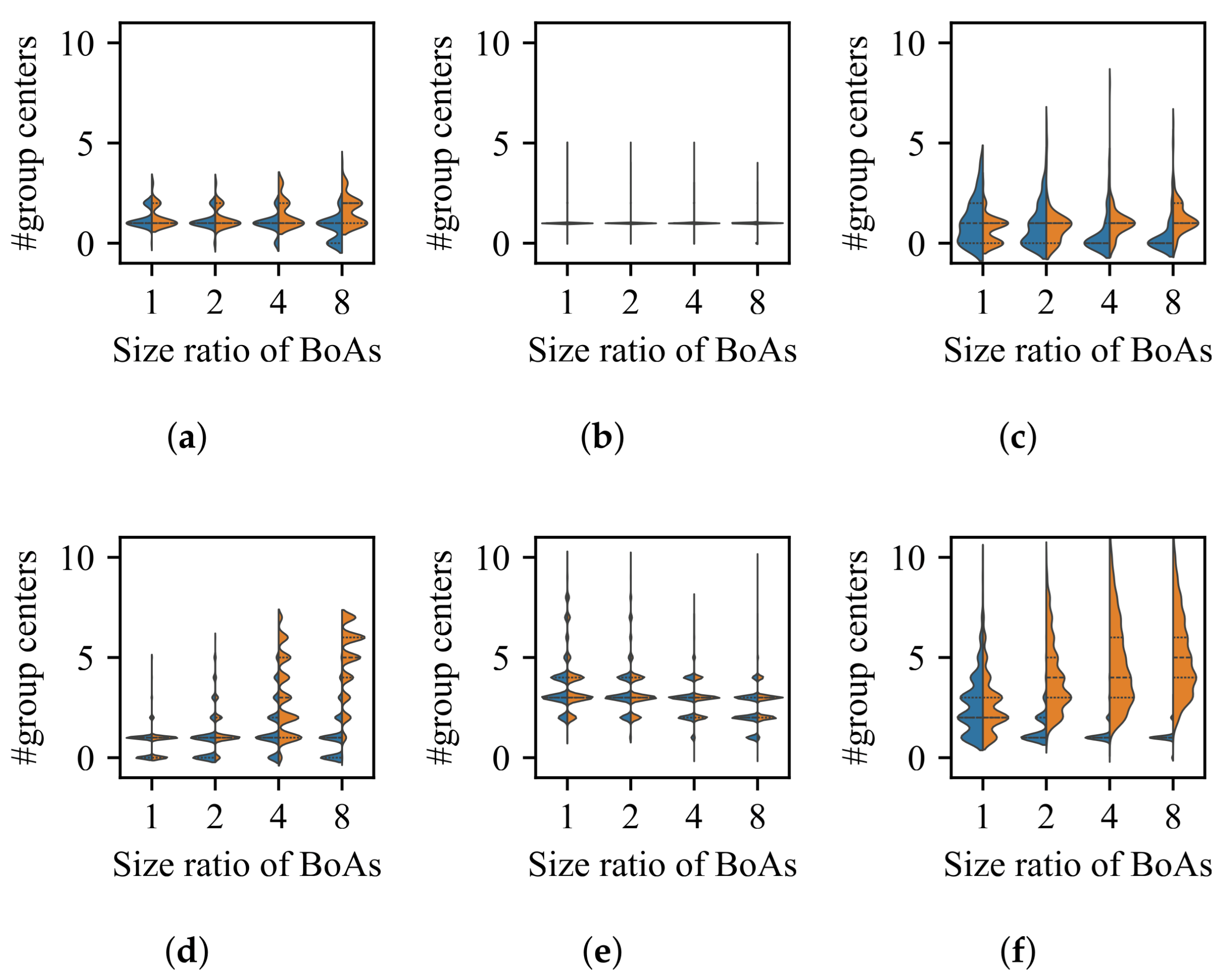
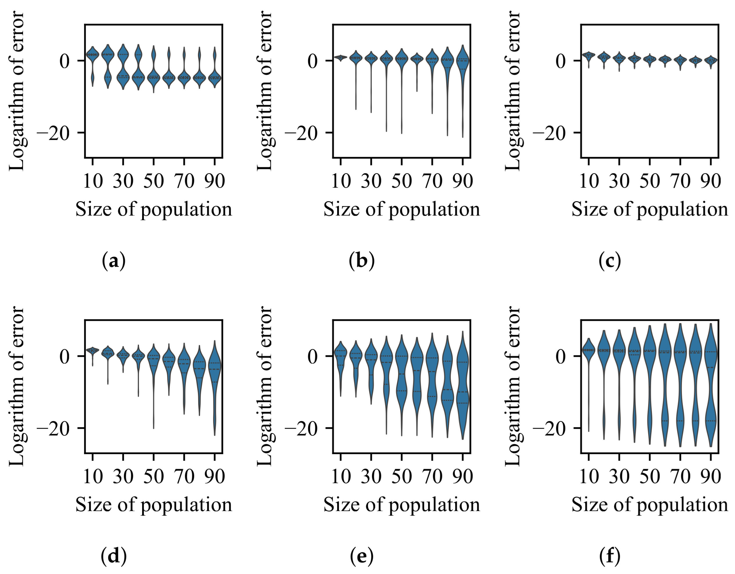
  The capability of the clustering with an adaptive number of groups technique can be enhanced by increasing the population size. While it is relatively straightforward for the adaptive clustering methods employed in current EC methods that use this technique to identify the presence of more challenging optima, there is a need for more balanced strategies to distribute function evaluations between these and other easily discoverable optima.

In addition to the above findings, a significant contribution of this paper is the demonstration, using the benchmark problems generated by Free Peaks, that the performance and behavioral nuances of EC methods in the BoAs of desired optima can be clearly distinguished from those in other BoAs. This allows for an effective verification of whether the purported disadvantages addressed by a given method are indeed resolved.

However, much work remains to be undertaken in the study of niching methods. Given that the search space may comprise BoAs of numerous local optima, a well-suited divide-and-conquer strategy, along with a logical sequence for “dividing” or “conquering,” can also aid in enhancing the global efficiency of identifying desired optima of lower attractiveness. Research efforts in this domain using current EC methods remain an urgent area for further investigation.

References

1. Bu, C.; Luo, W.; Yue, L. Continuous dynamic constrained optimization with ensemble of locating and tracking feasible regions strategies. IEEE Trans. Evol. Comput. 2016, 21, 14–33. [Google Scholar] [CrossRef]
2. Liang, J.J.; Yue, C.; Qu, B.Y. Multimodal multi-objective optimization: A preliminary study. In Proceedings of the 2016 IEEE Congress on Evolutionary Computation (CEC), Vancouver, BC, Canada, 24–29 July 2016; pp. 2454–2461. [Google Scholar]
3. Weise, T.; Chiong, R.; Tang, K. Evolutionary optimization: Pitfalls and booby traps. J. Comput. Sci. Technol. 2012, 27, 907–936. [Google Scholar] [CrossRef]
4. Baketarić, M.; Mernik, M.; Kosar, T. Attraction basins in metaheuristics: A systematic mapping study. Mathematics 2021, 9, 3036. [Google Scholar] [CrossRef]
5. Li, X.; Engelbrecht, A.; Epitropakis, M.G. Benchmark Functions for CEC’2013 Special Session and Competition on Niching Methods for Multimodal Function Optimization; Technical Report; Evolutionary Computation and Machine Learning Group, RMIT University: Melbourne, VIC, Australia, 2013. [Google Scholar]
6. Qu, B.; Liang, J.J.; Wang, Z.; Chen, Q.; Suganthan, P.N. Novel benchmark functions for continuous multimodal optimization with comparative results. Swarm Evol. Comput. 2016, 26, 23–34. [Google Scholar] [CrossRef]
7. Ahrari, A.; Deb, K.; Preuss, M. Multimodal optimization by covariance matrix self-adaptation evolution strategy with repelling subpopulations. Evol. Comput. 2017, 25, 439–471. [Google Scholar] [CrossRef]
8. Ahrari, A.; Deb, K. A novel class of test problems for performance evaluation of niching methods. IEEE Trans. Evol. Comput. 2017, 22, 909–919. [Google Scholar] [CrossRef]
9. Li, C.; Nguyen, T.T.; Zeng, S.; Yang, M.; Wu, M. An open framework for constructing continuous optimization problems. IEEE Trans. Cybern. 2018, 49, 2316–2330. [Google Scholar] [CrossRef]
10. Goldberg, D.E.; Richardson, J. Genetic algorithms with sharing for multimodal function optimization. In Genetic Algorithms and Their Applications, Proceedings of the Second International Conference on Genetic Algorithms, Cambridge, MA, USA, 28–31 July 1987; Lawrence Erlbaum: Hillsdale, NJ, USA, 1987; Volume 4149. [Google Scholar]
11. Pétrowski, A. A clearing procedure as a niching method for genetic algorithms. In Proceedings of the IEEE International Conference on Evolutionary Computation, Nagoya, Japan, 20–22 May 1996; pp. 798–803. [Google Scholar]
12. Tsutsui, S.; Fujimoto, Y.; Ghosh, A. Forking genetic algorithms: GAs with search space division schemes. Evol. Comput. 1997, 5, 61–80. [Google Scholar] [CrossRef]
13. Li, J.P.; Balazs, M.E.; Parks, G.T.; Clarkson, P.J. A species conserving genetic algorithm for multimodal function optimization. Evol. Comput. 2002, 10, 207–234. [Google Scholar] [CrossRef]
14. Wei, Z.; Gao, W.; Li, G.; Zhang, Q. A penalty-based differential evolution for multimodal optimization. IEEE Trans. Cybern. 2021, 52, 6024–6033. [Google Scholar] [CrossRef]
15. Ursem, R.K. Multinational evolutionary algorithms. In Proceedings of the 1999 Congress on Evolutionary Computation-CEC99, Washington, DC, USA, 6–9 July 1999; Volume 3, pp. 1633–1640. [Google Scholar]
16. Yao, J.; Kharma, N.; Zhu, Y.Q. On clustering in evolutionary computation. In Proceedings of the 2006 IEEE International Conference on Evolutionary Computation, Vancouver, BC, Canada, 16–21 July 2006; pp. 1752–1759. [Google Scholar]
17. Stoean, C.; Preuss, M.; Stoean, R.; Dumitrescu, D. Multimodal optimization by means of a topological species conservation algorithm. IEEE Trans. Evol. Comput. 2010, 14, 842–864. [Google Scholar] [CrossRef]
18. Maree, S.C.; Alderliesten, T.; Thierens, D.; Bosman, P.A.N. Real-valued evolutionary multi-modal optimization driven by hill-valley clustering. In Proceedings of the Genetic and Evolutionary Computation Conference, GECCO’18, Kyoto, Japan, 15–19 July 2018; Association for Computing Machinery: New York, NY, USA, 2018; pp. 857–864. [Google Scholar]
19. Thomsen, R. Multimodal optimization using crowding-based differential evolution. In Proceedings of the 2004 Congress on Evolutionary Computation, Portland, OR, USA, 19–23 June 2004; Volume 2, pp. 1382–1389. [Google Scholar]
20. Epitropakis, M.G.; Plagianakos, V.P.; Vrahatis, M.N. Finding multiple global optima exploiting differential evolution’s niching capability. In Proceedings of the 2011 IEEE Symposium on Differential Evolution (SDE), Paris, France, 11–15 April 2011; pp. 1–8. [Google Scholar]
21. Li, X. Niching without niching parameters: Particle swarm optimization using a ring topology. IEEE Trans. Evol. Comput. 2009, 14, 150–169. [Google Scholar]
22. Qu, B.Y.; Suganthan, P.N.; Das, S. A distance-based locally informed particle swarm model for multimodal optimization. IEEE Trans. Evol. Comput. 2012, 17, 387–402. [Google Scholar] [CrossRef]
23. Qu, B.Y.; Suganthan, P.N.; Liang, J.J. Differential evolution with neighborhood mutation for multimodal optimization. IEEE Trans. Evol. Comput. 2012, 16, 601–614. [Google Scholar] [CrossRef]
24. Gao, W.; Yen, G.G.; Liu, S. A cluster-based differential evolution with self-adaptive strategy for multimodal optimization. IEEE Trans. Cybern. 2014, 44, 1314–1327. [Google Scholar] [CrossRef] [PubMed]
25. Wang, K.; Gong, W.; Deng, L.; Wang, L. Multimodal optimization via dynamically hybrid niching differential evolution. Knowl.-Based Syst. 2022, 238, 107972. [Google Scholar] [CrossRef]
26. Preuss, M. Niching the CMA-ES via nearest-better clustering. In Proceedings of the 12th Annual Conference Companion on Genetic and Evolutionary Computation, Portland, OR, USA, 7–11 July 2010; pp. 1711–1718. [Google Scholar]
27. Li, L.; Tang, K. History-based topological speciation for multimodal optimization. IEEE Trans. Evol. Comput. 2015, 19, 136–150. [Google Scholar] [CrossRef]
28. Li, C.; Nguyen, T.T.; Yang, M.; Mavrovouniotis, M.; Yang, S. An adaptive multi-population framework for locating and tracking multiple optima. IEEE Trans. Evol. Comput. 2016, 4, 590–605. [Google Scholar] [CrossRef]
29. Cheng, R.; Li, M.; Li, K.; Yao, X. Evolutionary multiobjective optimization-based multimodal optimization: Fitness landscape approximation and peak detection. IEEE Trans. Evol. Comput. 2017, 22, 692–706. [Google Scholar] [CrossRef]
30. Wang, Z.J.; Zhan, Z.H.; Lin, Y.; Yu, W.J.; Wang, H.; Kwong, S.; Zhang, J. Automatic niching differential evolution with contour prediction approach for multimodal optimization problems. IEEE Trans. Evol. Comput. 2019, 24, 114–128. [Google Scholar] [CrossRef]
31. Jiang, Y.; Zhan, Z.; Tan, K.C.; Zhang, J. Optimizing niche center for multimodal optimization problems. IEEE Trans. Cybern. 2023, 53, 2544–2557. [Google Scholar] [CrossRef] [PubMed]
32. Li, Y.; Huang, L.; Gao, W.; Wei, Z.; Huang, T.; Xu, J.; Gong, M. History information-based hill-valley technique for multimodal optimization problems. Inf. Sci. 2023, 631, 15–30. [Google Scholar] [CrossRef]
33. Wang, J.; Li, C.; Zeng, S.; Yang, S. History-guided hill exploration for evolutionary computation. IEEE Trans. Evol. Comput. 2023, 27, 1962–1975. [Google Scholar] [CrossRef]
34. De Jong, K.A. An Analysis of the Behavior of a Class of Genetic Adaptive Systems. Ph.D. Thesis, University of Michigan, Ann Arbor, MI, USA, 1975. [Google Scholar]
35. Deb, K.; Pratap, A.; Agarwal, S.; Meyarivan, T. A fast and elitist multiobjective genetic algorithm: NSGA-II. IEEE Trans. Evol. Comput. 2002, 6, 182–197. [Google Scholar] [CrossRef]
36. Hansen, N.; Ostermeier, A. Completely derandomized self-adaptation in evolution strategies. Evol. Comput. 2001, 9, 159–195. [Google Scholar] [CrossRef]
37. Storn, R.; Price, K. Differential evolution—A simple and efficient heuristic for global optimization over continuous spaces. J. Glob. Optim. 1997, 11, 341–359. [Google Scholar] [CrossRef]
38. Zambrano-Bigiarini, M.; Clerc, M.; Rojas, R. Standard particle swarm optimisation 2011 at CEC-2013: A baseline for future PSO improvements. In Proceedings of the 2013 IEEE Congress on Evolutionary Computation, Cancun, Mexico, 20–23 June 2013; pp. 2337–2344. [Google Scholar]
39. Suganthan, P.N.; Hansen, N.; Liang, J.J.; Deb, K.; Chen, Y.P.; Auger, A.; Tiwari, S. Problem Definitions and Evaluation Criteria for the CEC 2005 Special Session on Real-Parameter Optimization; Technical Report 2005005; Kanpur Genetic Algorithms Laboratory, IIT Kanpur: Kanpur, India, 2005. [Google Scholar]
40. Beyer, H.G.; Sendhoff, B. Covariance matrix adaptation revisited—The CMSA evolution strategy–. In Proceedings of the International Conference on Parallel Problem Solving from Nature, Dortmund, Germany, 13–17 September 2008; Springer: Berlin/Heidelberg, Germany, 2008; pp. 123–132. [Google Scholar]
Figure 1. Illustration of space partitioning in Free Peaks. The left subfigure shows the four subspaces Ω 1 , , Ω 4 subdivided from a 2D bounded search space. The right subfigure shows the binary tree recording the process of partitioning, where each circular node represents a bisection.
Information 16 00583 g001
Figure 2. Contour lines of fitness landscapes of four problems with two decision variables, x 1 and x 2 , with the size ratios of the BoAs of two global optima set to (a) 1, (b) 2, (c) 4, and (d) 8, respectively.
Information 16 00583 g002
Figure 3. Distributions of fitness errors for two global optima over 100 runs of (a) SBX-GA, (b) DE/rand/1, (c) CMA-ES, and (d) SPSO-2011 on problems with the size ratios of the BoAs of the two global optima set to 1, 2, 4, and 8, respectively.
Information 16 00583 g003
Figure 4. Contour lines of fitness landscapes of four problems with two decision variables, x 1 and x 2 , with the peak function for one global optimum set to (a) s 1 , (b) s 9 , (c) s 5 , and (d) s 10 , respectively, while the peak function for the other global optimum remains s 1 .
Information 16 00583 g004
Figure 5. Fitness distributions of 10,000 uniform samples of peak functions s 1 , s 9 , s 5 , and s 10 .
Information 16 00583 g005
Figure 6. Distributions of fitness errors for two global optima over 100 runs of (a) SBX-GA, (b) DE/rand/1, (c) CMA-ES, and (d) SPSO-2011 on problems with the peak function for the second global optimum set to s 1 , s 9 , s 5 , and s 10 , respectively.
Information 16 00583 g006
Figure 7. Contour lines of fitness landscapes of four problems with two decision variables, x 1 and x 2 , with the distances between the two global optima set to (a) 1, (b) 2, (c) 3, and (d) 4 times the distance between two nearest local optima, respectively.
Information 16 00583 g007
Figure 8. Distributions of fitness errors for two global optima over 100 runs of (a) SBX-GA, (b) DE/rand/1, (c) CMA-ES, and (d) SPSO-2011 on problems with the distance between the two global optima set to 1, 2, 3, and 4, respectively.
Information 16 00583 g008
Figure 9. Contour lines of fitness landscapes of four problems with two decision variables, x 1 and x 2 , with the distances between the global optimum and the deceptive local optimum set to (a) 1, (b) 3, (c) 5, and (d) 7 times the distance between two nearest local optima, respectively.
Information 16 00583 g009
Figure 10. Distributions of fitness errors for the global optimum over 100 runs of (a) SBX-GA, (b) DE/rand/1, (c) CMA-ES, and (d) SPSO-2011 on problems with the distances between the global optimum and the deceptive local optimum set to 1, 3, 5, and 7, respectively.
Information 16 00583 g010
Figure 11. The average fitness error of LRDE, with the radius of repulsion ranging from 0.05 to 0.95, for the first global optimum over 100 runs on problems from the benchmark scenario with varying size ratios of the two global optima’s BoAs.
Information 16 00583 g011
Figure 12. Distributions of values of (a) taboo distances set in RS-CMSA or (b) penalty radii set in PMODE on problems from the benchmark scenario with varing size ratios of the two global optima’s BoAs.
Information 16 00583 g012
Figure 13. Distributions of fitness errors for two global optima over 100 runs of (a) RS-CMSA and (b) PMODE on problems with the size ratio of BoAs of the two global optima set to 1, 2, 4, and 8, respectively.
Information 16 00583 g013
Figure 14. Average fitness error of LRDE, with the radius of repulsion ranging from 0.05 to 0.95, for the first global optimum over 100 runs on problems with the size ratio of the two global optima’s BoAs ranging from 10 to 100.
Information 16 00583 g014
Figure 15. Distributions of threshold distance values for radial repulsion for (a) RS-CMSA and (b) PMODE for two global optima over 100 runs on problems with the size ratio of the BoAs of the two global optima set to 10, 40, 70, and 100, respectively.
Information 16 00583 g015
Figure 16. Distributions of fitness errors of (a) RS-CMSA and (b) PMODE for two global optima over 100 runs on problems with the size ratio of the BoAs of two global optima set to 10, 40, 70, and 100, respectively.
Information 16 00583 g016
Figure 17. Average fitness errors for the first global optimum over 100 runs of HVES on the problem with two global optima of the same peak function, with variation in (a) the number of gradations and the number of samples, (b) the size ratio of the BoAs and the number of samples, and (c) the size ratio of the BoAs and the number of gradations.
Information 16 00583 g017
Figure 18. Distributions of fitness errors for two global optima over 100 runs of (a) TSC2, (b) HillVallEA, and (c) HVES on problems with the size ratio of the BoAs of the two global optima set to 1, 2, 4, and 8, respectively.
Information 16 00583 g018
Figure 19. Distributions of values for the number of samples when running HillVallEA on problems with the size ratio of the BoAs of the two global optima set to 1, 2, 4, and 8.
Information 16 00583 g019
Figure 20. Average fitness errors for the first global optimum over 100 runs of kNPSO on the problem with two global optima of the same peak function, varying (a) the number of neighbors and the population size, and (b) the size ratio of BoAs and the population size.
Information 16 00583 g020
Figure 21. Distributions of fitness errors for two global optima over 100 runs of (a) CDE, (b) DE/nrand/1, (c) NCDE, (d) R2PSO, (e) LIPS, and (f) kNPSO on problems with the size ratio of the BoAs of the two global optima set to 1, 2, 4, and 8, respectively.
Information 16 00583 g021
Figure 22. Distributions of fitness errors for two global optima over 100 runs of (a) NSDE, (b) self-CCDE, (c) self-CSDE, and (d) DHNDE on problems with the size ratio of the BoAs of the two global optima set to 1, 2, 4, and 8, respectively.
Information 16 00583 g022
Figure 23. Distributions of fitness errors for two global optima over 100 runs of DHNDE with the population size set to 7 on problems with the size ratio of the BoAs of the two global optima set to 1, 2, 4, and 8, respectively.
Information 16 00583 g023
Figure 24. Average fitness errors for the first global optimum over 100 runs of NSDE on the problem with two global optima of the same peak function, varying (a) the group size and the population size, and (b) size the ratio of the BoAs and the population size.
Information 16 00583 g024
Figure 25. Distributions of fitness errors for two global optima over 100 runs of (a) NEA2 without restart, (b) HTS-CDE, (c) EMO-MMO, (d) ANDE, (e) NCD-DE, and (f) ESPDE on problems with the size ratio of the BoAs of the two global optima set to 1, 2, 4, and 8, respectively.
Information 16 00583 g025
Figure 26. Distributions of numbers of group centers in BoAs of two global optima over 100 runs of (a) NEA2 without restart, (b) HTS-CDE, (c) EMO-MMO, (d) ANDE, (e) NCD-DE, and (f) ESPDE on problems with the size ratio of the BoAs of the two global optima set to 1, 2, 4, and 8, respectively.
Information 16 00583 g026
Figure 27. Variation in the distribution of fitness errors for the first global optimum over 100 runs of (a) NEA2 without restart, (b) ANDE, (c) NCD-DE, (d) HTS-CDE, (e) ESPDE, and (f) EMO-MMO on problems with the size ratio of the BoAs of the two global optima set to 20, with the population size varing from 10 to 90.
Information 16 00583 g027