A Lightweight Multi-Frequency Feature Fusion Network with Efficient Attention for Breast Tumor Classification in Pathology Images

Abstract

The intricate and complex tumor cell morphology in breast pathology images is a key factor for tumor classification. This paper proposes a lightweight breast tumor classification model with multi-frequency feature fusion (LMFM) to tackle the problem of inadequate feature extraction and poor classification performance. The LMFM utilizes wavelet transform (WT) for multi-frequency feature fusion, integrating high-frequency (HF) tumor details with high-level semantic features to enhance feature representation. The network’s ability to extract irregular tumor characteristics is further reinforced by dynamic adaptive deformable convolution (DADC). The introduction of the token-based Region Focus Module (TRFM) reduces interference from irrelevant background information. At the same time, the incorporation of a linear attention (LA) mechanism lowers the model’s computational complexity and further enhances its global feature extraction capability. The experimental results demonstrate that the proposed model achieves classification accuracies of 98.23% and 97.81% on the BreaKHis and BACH datasets, with only 9.66 M parameters.

1. Introduction

Malignant breast tumors are among the most prevalent types of cancer in women, and their incidence has shown a marked upward trend in recent years [1]. Early diagnosis and intervention are critical for reducing breast cancer mortality. When a mass or nodule is detected in the breast during clinical examination, medical imaging modalities are employed to assess whether the lesion is malignant. Different imaging techniques, including computed tomography (CT), magnetic resonance imaging (MRI), and ultrasound, provide clinicians with macroscopic information regarding the location, size, and shape of breast tumors. Once the tumor site is identified, a biopsy is performed to confirm the diagnosis and to determine the tumor type and its growth characteristics within the breast tissue. In the field of clinical diagnosis, histopathological examination is widely recognized as the gold standard [2] for the definitive diagnosis of breast cancer. Pathologists typically evaluate breast tissue images under a microscope by examining the morphological characteristics of cells, a process that is not only time-consuming and labor-intensive but also subject to inter-observer variability. Therefore, developing an efficient and accurate breast tumor classification method holds significant clinical value.

The complex spatial structures and texture details within breast tissue are critical factors for tumor classification. Therefore, it is essential to integrate local features and global contextual information in tissue images to make accurate judgments. Deep learning has made significant advancements in computer vision. Convolutional neural networks (CNNs) can automatically extract fine-grained features from images, such as edges and textures, through local receptive fields and have found widespread application in tumor detection at different levels. Musfequa et al. [3]. designed a convolutional module guided by the Convolutional Block Attention Module (CBAM), which effectively highlights critical features while suppressing irrelevant information. In addition, a Deep Broad block was introduced to enhance the network’s adaptability to images with varying resolutions. The model achieved an accuracy of over 98.67% across all four magnification factors on the BreaKHis dataset. However, its computational complexity, measured in Floating Point Operations (FLOPS), reached 2.83 G, which poses challenges for deployment on mobile devices. Xu et al. [4] proposed an improved high-precision breast cancer classification approach based on a modified CNN. They introduced three different variants of the MFSCNET model, which differ in terms of the insertion positions and the number of Squeeze-and-Excitation (SE) modules. However, due to the fixed receptive field of CNNs, it is difficult to recognize the complex morphological variations among different tumor types. Consequently, their model achieved an accuracy of only 94.36% at 100× magnification. Furthermore, the computational cost, measured in FLOPS, reached as high as 2.17 G. Rajendra Babu et al. [5] designed a bidirectional recurrent neural network (BRNN) that leverages a pre-trained ResNet50 to extract coarse feature information from breast images. The network employs a residual branch as a collaborative module to ensure that critical features are retained and utilizes a Gated Recurrent Unit (GRU) to analyze spatial dependencies within tumor characteristics. BRNN effectively integrates multi-branch features, achieving an average classification accuracy of 97.25% on the BreaKHis dataset. However, due to its multi-branch architecture and feature fusion strategy, BRNN requires substantial computational resources, with FLOPS reaching approximately 8G, thereby limiting its inference efficiency. Liu et al. [6] developed a model based on the EfficientNetB0 architecture, incorporating multi-branch convolutions and Squeeze-and-Excitation (SE) channel attention mechanisms to automatically focus on lesion regions at different scales, thereby enhancing the extraction of tumor features across various magnifications. The model achieved a binary classification accuracy of 95.34% and a multi-class classification accuracy of 95.97% on the BreaKHis dataset. However, this increased computational complexity and introduced unnecessary or redundant information, resulting in a parameter count of 49.85 M—approximately ten times that of the baseline network. Mahdavi [7] improved conventional CNN architectures by replacing the ReLU activation function with K-winners, adopting the sparse random initialization of weights, and incorporating the k-nearest neighbors algorithm for tumor classification. These modifications enhanced the noise robustness of the CNN architecture. Wingates et al. [8] analyzed the performance of breast tumor classification using transfer learning across various CNN architectures. Among these, the ResNetV1-50 model achieved the highest computational complexity, with 4.1B FLOPS and 25.6 M parameters (Params), but only attained an accuracy of 92.53%. In contrast, architectures such as EfficientNet and MobileNet achieved classification accuracies exceeding 93% while maintaining much lower model complexity. These findings suggest that selecting a lightweight CNN model capable of delivering relatively high accuracy is more cost-effective for practical deployment. However, the F1-Scores of most CNN architectures fluctuate around 90%, indicating a potential issue of class imbalance in classification performance across different categories.

Due to the limited receptive field of convolution operations in CNNs, deeper network layers can only capture certain low-level information from the initial layers, resulting in the loss of global contextual relationships within features. The Vision Transformer (ViT) [9] partitions images into patch tokens and incorporates positional encodings [10], enabling the transformer architecture to capture the spatial positional information of different regions. By applying a self-attention mechanism across the entire image, the model can capture long-range dependencies between arbitrary regions and extract global feature representations with rich semantic information. Shiri et al. [11] leveraged a pre-trained ViT to effectively process spatial information in histopathological images, utilizing supervised contrastive loss to enhance the discriminative capability of salient features within samples. To establish comprehensive spatial feature relationships, transformer models must exchange information between every patch, leading to excessive network complexity for Vision Transformers. Specifically, the Params and FLOPS reach 85.8 M and 55.3 G, respectively. The substantial computational burden incurred in pursuit of higher classification accuracy, at the expense of network efficiency, renders this approach unsuitable for deployment on mobile devices. Swin Transformer addresses this issue by partitioning the feature map into multiple non-overlapping regions of patch size, where local attention is first computed within each window. Subsequently, cross-region information exchange is performed to enhance global modeling capabilities. This hierarchical approach effectively reduces network complexity to a certain extent while maintaining competitive performance. Tummala et al. [12] conducted multi-class breast tumor classification by ensembling four Swin Transformers, achieving an average classification accuracy of 93.9%, which surpasses most baseline CNN architectures. However, due to the window partitioning strategy, the capability to suppress background noise remains limited. However, it is noteworthy that Swin Transformer still requires 27.5 G Params, which exceeds those required by the vast majority of CNN architectures.

Currently, features extracted by a single network often fail to capture the differences between various breast tumor categories adequately. To effectively combine the respective strengths of both architectures, Zhang et al. [13] proposed a parallel weighted ensemble of Swin Transformer and CNN for multi-class breast tumor classification. By integrating both local and global features of breast tumors, they reached a classification accuracy of 96.63%. Sreelekshmi et al. [14] first extracted local breast tumor features using depthwise separable convolution (DSC) and then input these local features into a Swin Transformer framework to capture global information. The experimental results demonstrated that the SwinCNN architecture outperformed single-network models, improving classification accuracy on the BreaKHis dataset by up to 5.95 % and on the BACH dataset by up to 5.16%. Wang et al. [15] innovatively proposed an LGVIT architecture, where a CNN extracts low-level breast tumor information to compensate for the Transformer’s limitations in local feature extraction. Subsequently, representative tokens from each window are processed through multi-head self-attention, facilitating the construction of cross-regional spatial information. However, its parallel integration inevitably leads to an increase in both the number of network Params and computational complexity. Additionally, the multi-branch structure introduces challenges in parameter tuning and may adversely affect convergence speed. Li et al. [16] ingeniously integrated the strengths of ConvNeXt and Swin Transformer, enabling the model to capture fine-grained local features of breast tissue while also extracting critical global contextual information. In addition, by enhancing edge and texture features from a frequency-domain perspective, their approach achieved classification accuracies of 91.15% and 93.62% on the BreaKHis and BACH datasets, respectively. The model contains 68.45 M Params and 9.24 G FLOPs. By modifying the depth and hierarchical structure of the original baseline, fusing both CNN and Transformer architectures, and introducing frequency-domain operators, the method not only improved model performance but also reduced computational complexity. Vaziri et al. [17] proposed recursive covariance computation and dimensionality reduction methods for EEG source localization, emphasizing the synergistic enhancement of feature representation capability and computational efficiency. Their approach reduced the computational workload by 66%, significantly improving the efficiency of the network. Although integrating CNN and Transformer architectures can enhance classification performance, direct fusion without explicit feature selection tends to introduce redundant information. Moreover, the varying importance of features across different scales and hierarchical levels during training with distinct architectures has not been adequately addressed. Mahdavi [18] achieved high-precision segmentation of high-dimensional tumors by designing a multi-level output architecture and integrating multiple loss functions, including cross-entropy, Dice, and KL-Divergence, in conjunction with regularization strategies. Khaniki et al. [19] incorporated a Feature Calibration Mechanism into Vision Transformers to calibrate multi-scale features. Furthermore, they employed Selective Cross-Attention to compute token correlations, enabling the selection of highly attentive features for global information construction. This strategy reduced network redundancy and enhanced the quality of feature extraction, resulting in a classification performance improvement of 3.92% compared to CNNs and 2.2% compared to standard ViT.

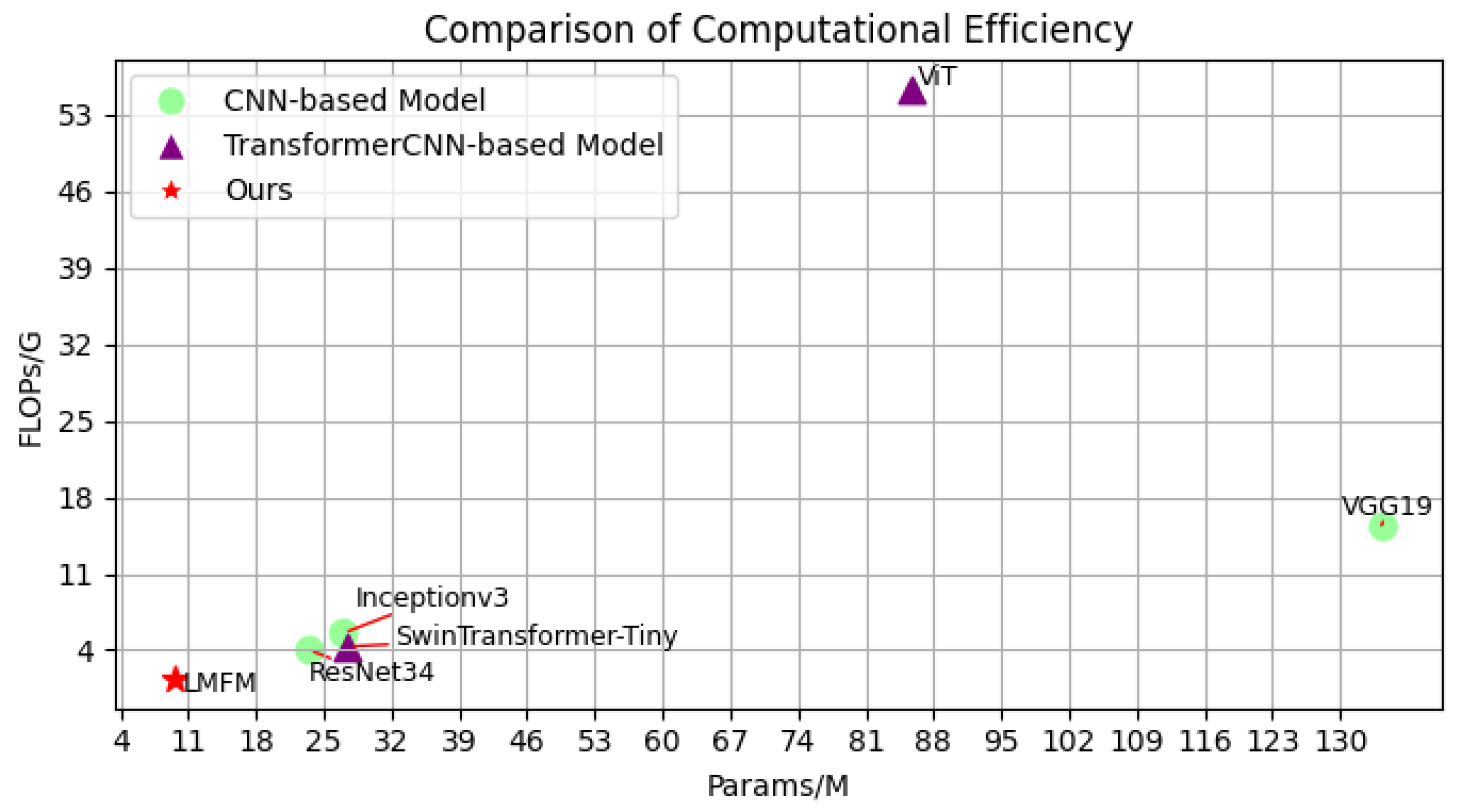
The above studies demonstrate that CNN and Transformer architectures can learn complementary strengths from each other, enabling the network to capture richer and more comprehensive image features. However, both CNN- and ViT-based architectures typically involve a large number of Params, requiring substantial computational resources and extended training times, which hinders their deployment on mobile or resource-constrained devices. Additionally, it is crucial to consider multi-level feature representations when dealing with complex breast tumor cell images. In current breast tumor classification methods, the low-frequency (LF) information of an image is primarily composed of structural features of tumor cells, while high-frequency (HF) information reflects intricate textural details. However, as the network depth increases, HF information is often smoothed or filtered out through repeated convolutions [20], further diminishing image detail. Finally, breast tumor datasets often contain irrelevant background regions that adversely impact classification accuracy. Moreover, the diverse cellular morphologies across different tumor types present additional challenges, as conventional convolutions extract features with fixed receptive field shapes, limiting their ability to adapt to the complex and varied structures in breast tumor images.

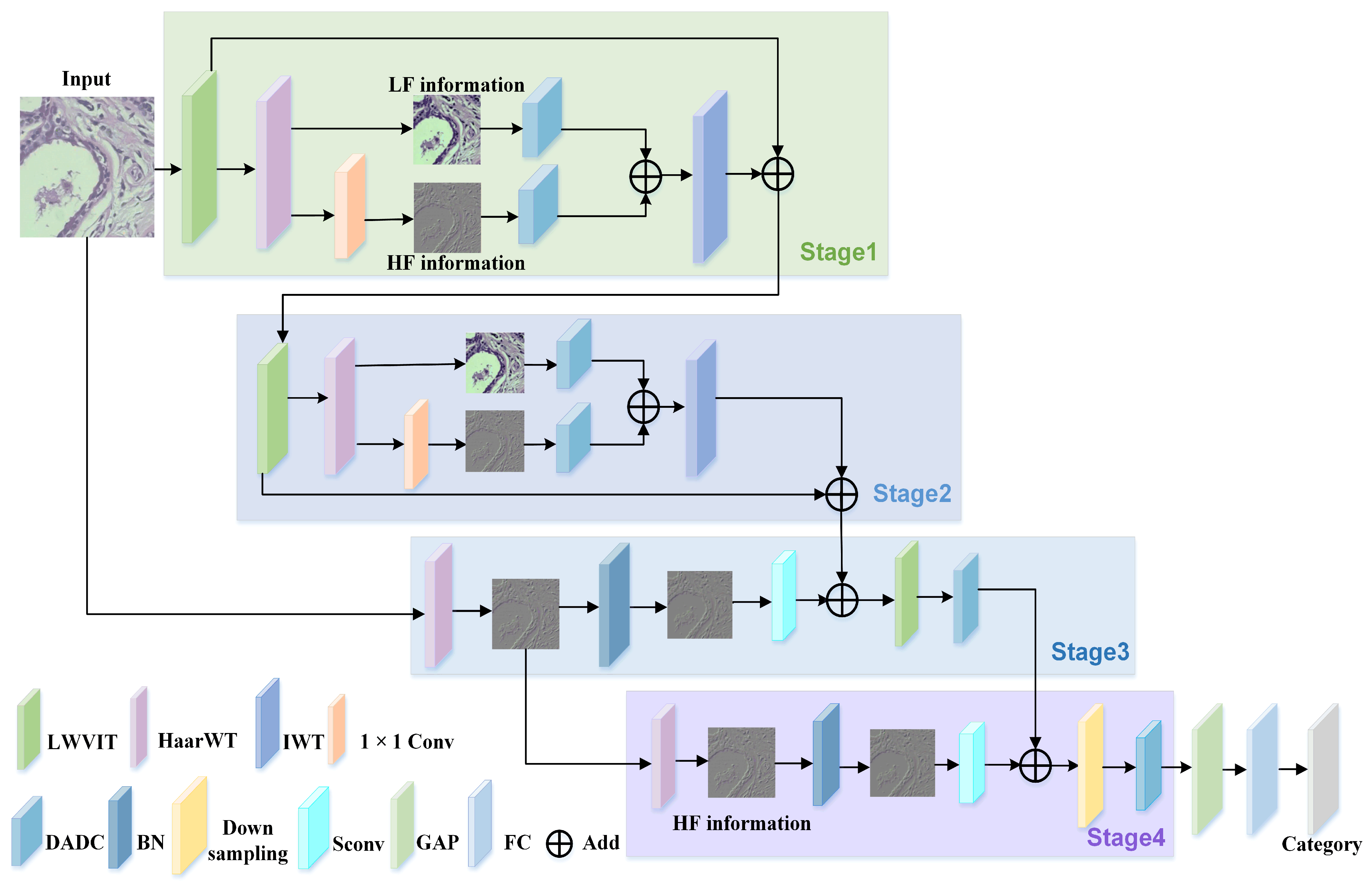
This paper proposes a lightweight multi-frequency feature fusion model (LMFM) for breast tumor classification to address the aforementioned challenges. The key contributions are as follows:

• To reduce information loss in breast tumor tissue cells, this paper employs wavelet transform (WT) to decompose input images into HF and LF components, enabling separate feature extraction at different levels and enhancing the interpretability of the resulting features.
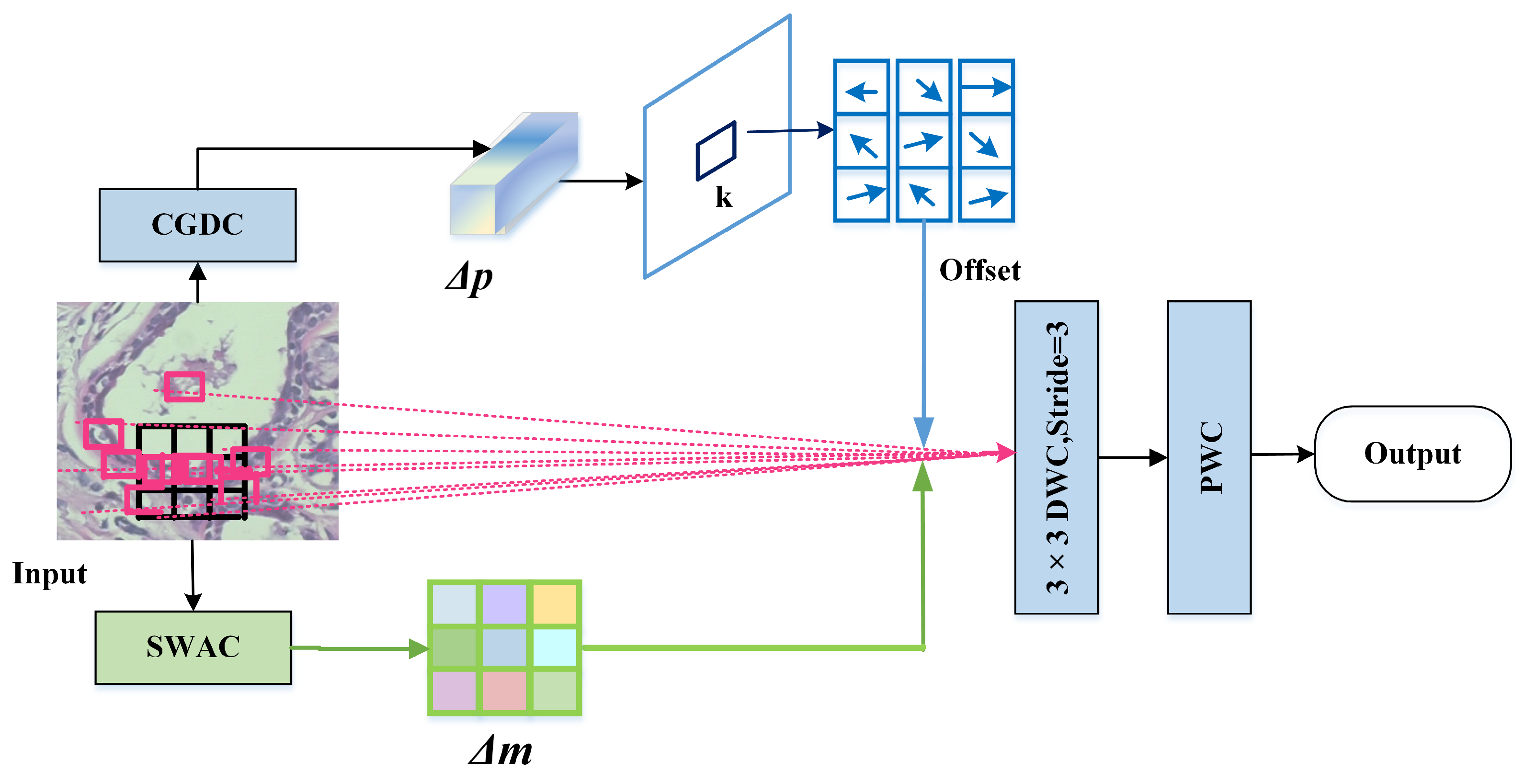
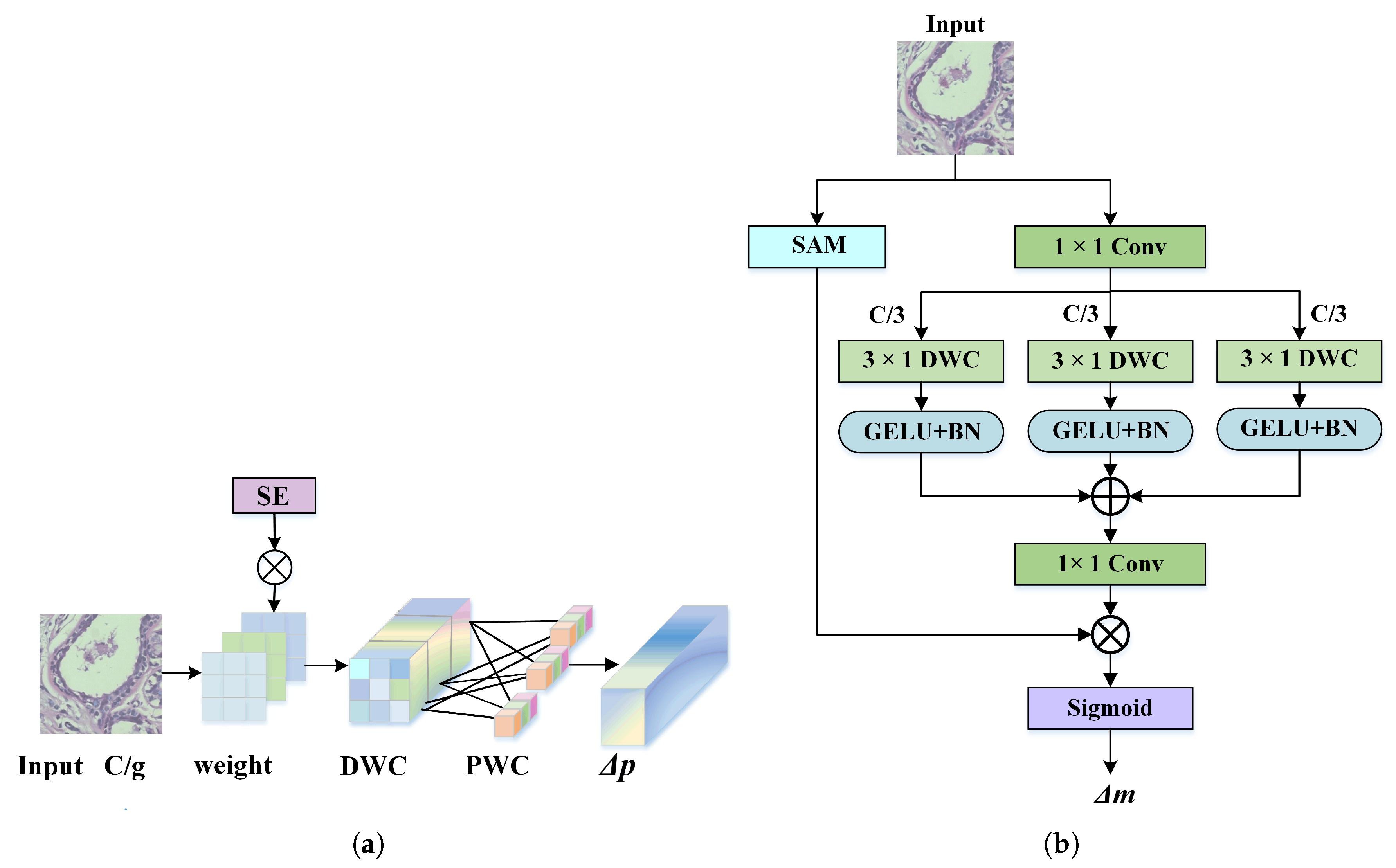
• This paper designs a dynamic adaptive deformable convolution (DADC) method combined with DSC to capture local detail features. Channel Weight Multi-Group Dynamic Convolution (CGDC) is introduced to distinguish inter-channel feature offset characteristics, and Spatial Weight Asymmetric Convolution (SWAC) is incorporated to enhance features in regions of interest. This effectively mitigates the limitations of conventional convolutions in modeling irregular tumor shapes.
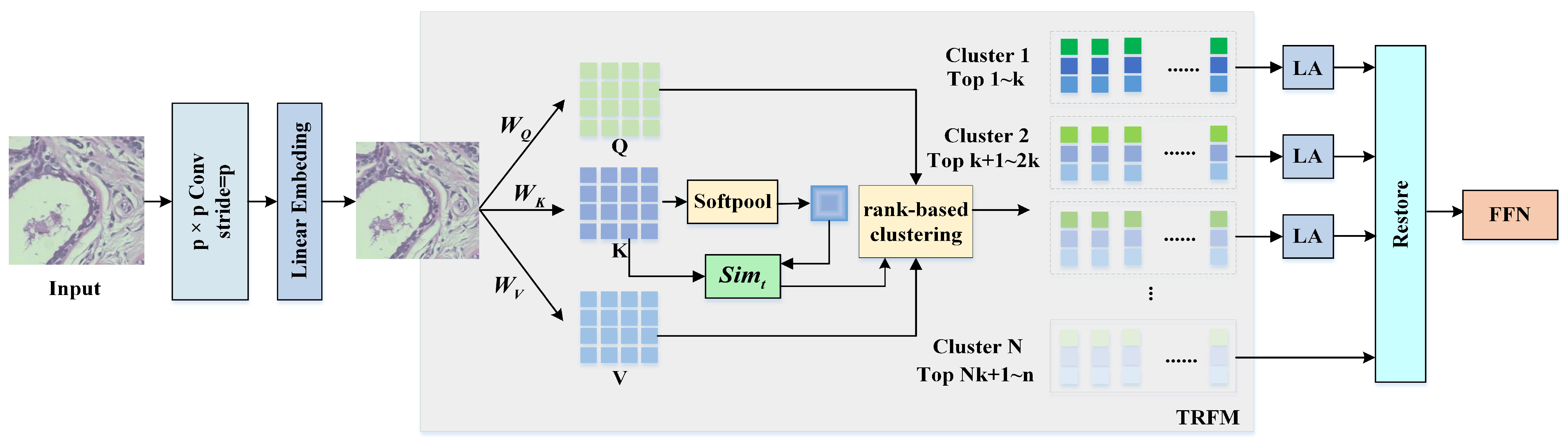
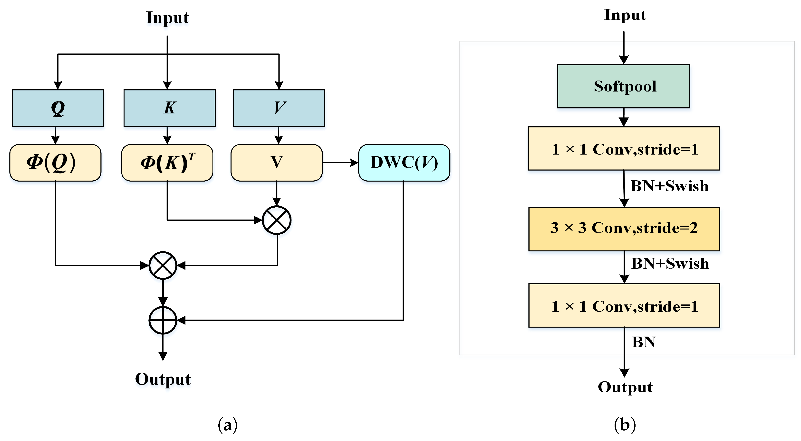
• To reduce interference from irrelevant background regions, this paper proposes a lightweight Vision Transformer (LWVIT) for spatial feature refinement. Tokens with rich semantic information (TRFM) are processed via a global self-attention mechanism, focusing primarily on the tumor and surrounding areas. Moreover, the conventional self-attention in Transformers is replaced with a linear attention (LA) computation, and the order of information exchange is reorganized to decrease network complexity.
• To further enhance the representation of local details in deep network layers, the original HF features of the image are incorporated into deeper layers, enhancing the model’s capacity to capture detailed information.

The LMFM model proposed in this study demonstrates superior accuracy and efficiency in breast tumor classification. Through efficient feature extraction and multi-frequency fusion, it enhances the recognition of tumor cell morphological characteristics, enabling not only the differentiation between benign and malignant tumors but also the precise identification of specific subtypes, thereby effectively reducing misdiagnosis in clinical practice. Its lightweight and efficient design makes it well-suited for resource-limited clinical settings, facilitating the broader adoption of breast cancer screening and improving diagnostic efficiency while reducing reliance on costly equipment. This, in turn, promotes the early detection and precise treatment of breast cancer in clinical practice.

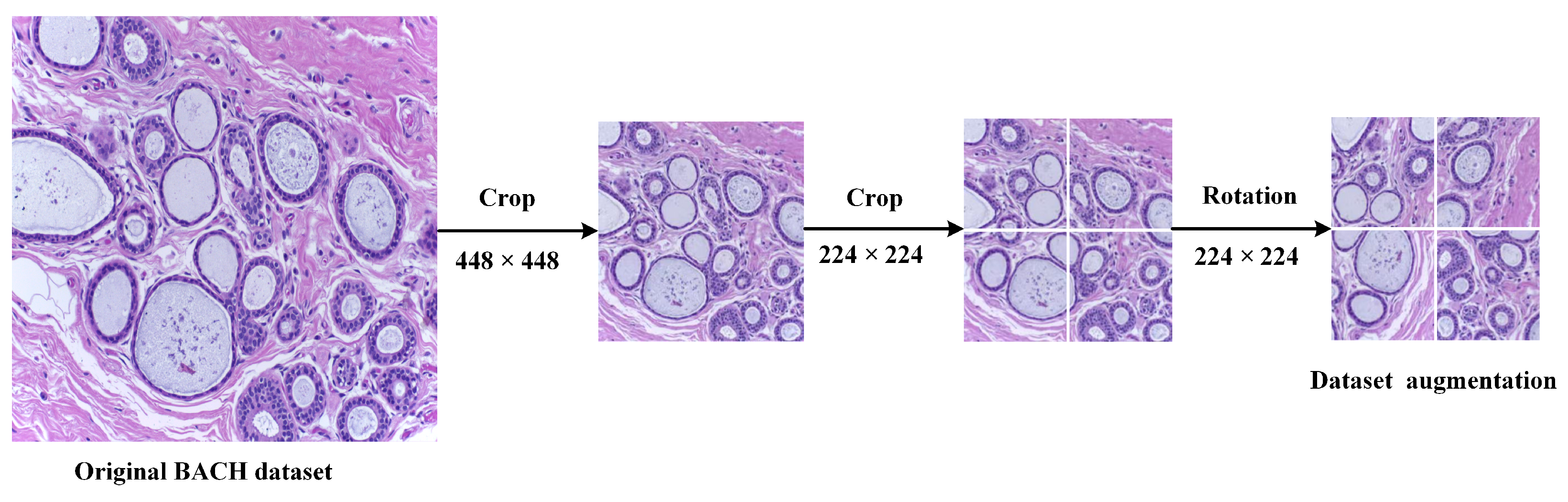
The remainder of this paper is organized as follows: Section 2 provides a description of the dataset and introduces a novel LMFM architecture along with its implementation. Subsequently, Section 3 presents the experiments and results analysis to validate the effectiveness of the proposed model. Finally, Section 4 concludes the paper and discusses future directions.

2. Materials and Methods

2.1. Dateset

Experiments for the LMFM were conducted on two breast pathology image datasets: BreaKHis and BACH. The BreaKHis dataset, released by Spanhol et al. in 2016, comprises breast tissue biopsy slides from 82 patients. All images were obtained from clinical studies and stained using hematoxylin and eosin (H&E). The dataset comprises a total of 7909 microscopic biopsy images, each with a resolution of $700\times 460$ pixels. These images are categorized into eight subtypes of benign and malignant tumors and were acquired at varying magnification levels. The distribution of tumor subtypes in the BreaKHis dataset is summarized in

Table 1. The composition of tumor types in the BreaKHis dataset.

Category	$40\times$	$100\times$	$200\times$	$400\times$	Total
Adenosis (AD)	114	113	111	106	444
Fibroadenoma (FA)	253	260	264	237	1014
Phyllodes_tumor (PT)	109	121	108	115	453
Tubular_adenoma (TA)	149	150	140	130	569
Ductal_carcinoma (DC)	864	903	896	788	3451
Lobular_carcinoma (LC)	156	170	163	137	626
Mucinous_carcinoma (MC)	205	222	196	169	792
Papillary_carcinoma (PC)	145	142	135	138	560
Total	1995	2081	2013	1820	7909

. The BACH dataset consists of 400 high-resolution ($2048\times 1536$ pixels) H&E-stained breast cancer pathology images. Each image was captured at 200× magnification, and the dataset is evenly divided into four categories: Normal, Benign, InSitu, and Invasive carcinoma, with 100 images per category, forming a balanced dataset.

The BreaKHis and BACH datasets employed in this paper are both derived from real clinical research. They are widely used by researchers internationally in the field of breast pathology image analysis. They are among the most representative publicly available datasets in this area. Specifically, the BreaKHis dataset covers a wide range of breast tumor types with varying resolutions, reflecting the diversity and complexity of pathological images encountered in clinical practice. This makes it well-suited for evaluating the model’s performance in fine-grained classification tasks. In contrast, the BACH dataset consists of high-resolution breast cancer histology images, which are more consistent with the quality requirements of practical clinical images. Therefore, conducting experiments on these two datasets provides strong evidence for the generalization capability of our proposed model in breast histopathological image classification.

2.2. Dateset Preprocessing

Due to potential variations in sample collection and staining time in the original datasets, the Vahadane algorithm [21] was employed to independently perform color normalization on each dataset, thereby eliminating staining differences. To mitigate noise interference and reduce the risk of model overfitting, this paper employs image normalization, random cropping, and random rotation for preprocessing and data augmentation on the BreaKHis dataset during training. These approaches enhance training stability and accelerate model convergence.

• Image Normalization: Each input value in the dataset is mapped to the range $\left[0, 1\right]$ using the image’s mean and standard deviation.
• Random Image Rotation: Images are randomly rotated within a range of $-{45}^{\circ }$ to $+{45}^{\circ }$.
• Random Cropping: Images are randomly cropped to a specified size. In this paper, all images are resized to $224\times 224$ pixels.

For the BACH dataset, the same preprocessing strategies as those applied to BreakHis were adopted. However, due to the limited number of samples, this paper first performed additional data augmentation in the BACH dataset to meet the data requirements of deep learning models and further reduce overfitting, as illustrated in Figure 1. Specifically, each original image was resized to $448\times 448$ pixels and then partitioned into four non-overlapping sub-images of $224\times 224$ pixels. Additional data augmentation was performed through random rotations, resulting in a fourfold increase in the total number of samples.

2.3. Methods

While CNN effectively extracts local features, they often fail to capture the global context in breast tumor classification. Transformers enhance global modeling but may weaken local feature extraction. This paper propose a novel LMFM architecture that fuses global and local features by integrating CNN and Transformer, enabling more comprehensive feature representation for complex breast tissue images. As shown in Figure 2, the LMFM specifically consists of LWVIT, WT, DADC, Sconv and Classifier.

The original image undergoes data augmentation before an LWVIT is used for global feature extraction. Subsequently, WT is applied to convert feature frequencies into LF and HF information. The features are then processed through DADC for local detail feature extraction and fusion. Afterward, inverse wavelet transform (IWT) maps the features back to the original feature map size, allowing for a larger receptive field in response to the input image. The feature extraction in the LMFM architecture consists of four layers, with the LMFM parameter settings given in

Table 2. LMFM specific parameters.

Model Stage	Output Feature Map Size	Specific Parameters
Input	$H\times W\times 3$	-
Stage 1	${\displaystyle \frac{H}{4}}\times {\displaystyle \frac{W}{4}}\times 4$	$\mathrm{LWVIT}$, $\mathit{p}=4$, $\mathit{k}=49$
		Haar WT
		$\mathrm{DADC}\times 2$, $\mathit{k}=3$, $\mathit{g}=8$
		IWT
Stage 2	${\displaystyle \frac{H}{8}}\times {\displaystyle \frac{W}{8}}\times 128$	$\mathrm{LWVIT}$, $\mathit{p}=2$, $\mathit{k}=49$
		Haar WT
		$\mathrm{DADC}\times 2$, $\mathit{k}=3$, $\mathit{g}=16$
		IWT
Stage 3	${\displaystyle \frac{H}{16}}\times {\displaystyle \frac{W}{16}}\times 256$	Haar WT, BN, $\mathrm{Sconv}$
		$\mathrm{LWVIT}$, $\mathit{p}=2$, $\mathit{k}=49$
		$\mathrm{DADC}\times 2$, $\mathit{k}=3$, $\mathit{g}=32$
Stage 4	${\displaystyle \frac{H}{32}}\times {\displaystyle \frac{W}{32}}\times 512$	Haar WT, BN, $\mathrm{Sconv}$
		Downsampling
		$\mathrm{DADC}\times 2$, $\mathit{k}=3$, $\mathit{g}=64$
Classifier	$1\times 8$	$GAP$
		$FC$, $\mathit{C}=8$

. As the network depth increases, the feature maps become more abstract, making capturing HF detailed information on breast tumors increasingly difficult. Therefore, in this work, HF information from the original image is injected into the last two layers for feature enhancement. Specifically, WT is first applied to the original image to obtain HF breast tumor features. The Sconv module then processes these HF features to match the network layer dimensions and is subsequently fused with the features extracted from the previous layer before being fed into the next feature extraction layer. In the final layer of the proposed network, an LWVIT is not employed; instead, a convolutional downsampling module with a kernel size of 3 × 3 and a stride of 2 is used to reduce the feature map size. Finally, a classifier is used to output the predicted breast tumor category label, thus completing the classification task. In summary, the LMFM achieves more comprehensive feature representations by combining the local information captured by the DADC with the global information extracted by the LWVIT.

2.3.1. WT Method

Convolutional layers in CNNs are typically biased toward responding to HF information, whereas LF features—such as tumor morphology and overall contours—are more consistent with human visual preferences [22]. To integrate the representational capabilities of both types of features, this paper employs Haar Wavelet Transform (HaarWT) [23], decomposing the input features into LF and HF components to capture the complementary aspects of image characteristics. HaarWT employs four filters to extract frequency components from images in the horizontal, vertical, and diagonal directions, capturing LF and HF information. The definitions of these filters are as follows:

$$f_{LL}={\displaystyle \frac{1}{2}}\left[\begin{array}{cc}1& 1\\ 1& 1\end{array}\right], f_{LH}={\displaystyle \frac{1}{2}}\left[\begin{array}{cc}1& -1\\ 1& -1\end{array}\right], f_{HL}={\displaystyle \frac{1}{2}}\left[\begin{array}{cc}1& 1\\ -1& -1\end{array}\right], f_{HH}={\displaystyle \frac{1}{2}}\left[\begin{array}{cc}1& -1\\ -1& 1\end{array}\right]$$

(1)

As shown in Figure 3, the original feature map undergoes two iterations of WT. For instance, a 3 × 3 convolution is applied to the LF band of the second-level wavelet domain. This approach utilizes only 9-parameter convolution to achieve a receptive field size of 12 × 12 in the input feature map X. After applying WT, the dimensions of the feature map are reduced by half. Following the feature extraction, a transposed convolution is employed to perform the IWT, restoring the feature map to its original size. This operation effectively increases the receptive field of the convolution while reducing the complexity of the network. The final output is denoted as

$$x=Con{v}^T\left(\left[f_{LL}, f_{LH}, f_{HL}, f_{HH}\right], \left[X_{LL}, X_{LH}, X_{HL}, X_{HH}\right]\right)$$

(2)

The LMFM achieves a receptive field size 6 × 6 by utilizing a first-level WT with a 3 × 3 convolutional kernel. Next, this paper will focus on the feature extraction and interaction of LF and HF information separately.

2.3.2. DADC Method

CNN has been widely applied in breast tumor detection because it can automatically extract detailed features such as edges and textures through local receptive fields. However, tumor regions in breast pathological images typically exhibit highly irregular shapes, as shown in Figure 4. Standard convolutional kernels employ weight sharing, yielding uniform responses to edges or structural features in all directions across the network. While this mechanism improves parameter efficiency, it inherently limits the sensitivity of standard convolutions to irregular structural patterns [24]. Additionally, standard convolutions extract features by sliding the kernel across the feature map in a fixed, translational manner without the ability to adjust adaptively to the directions and shapes of tumor boundaries. This frequently results in the extraction of irrelevant background information [25]. Moreover, the use of fixed square kernels (such as $3\times 3$) constrains the receptive field during feature extraction, making it challenging for the model to capture both fine details and global structural context simultaneously. This limitation impairs the network’s ability to distinguish subtle feature variations across different regions of breast tumor images. Therefore, standard convolution finds it inherently challenging to adapt to the morphological heterogeneity between different tumor regions and is insufficient for accurately capturing the complex characteristics of breast tumors. This paper replaces the standard convolution with DADC to address this issue. During network training, DADC adaptively adjusts the convolutional sampling positions based on the features of the breast tumor images.

Building upon the traditional deformable convolution DCNv2 [26], as illustrated in Figure 4, this paper introduces a SWAC module with spatial weight modulation into the convolutional kernel to adjust the amplitude of input features in different spatial locations, thereby enabling more precise control over the sampling range of the deformable convolution kernels. Since the generation of feature map offsets does not consider the diversity among different channels, this paper further design a CGDC module that incorporates a channel attention mechanism with DSC to improve the computation of convolutional offsets. After obtaining complex and diverse features of interest through the deformable kernels, local feature extraction is performed using 3 × 3 depthwise convolution (DWC) followed by 1 × 1 pointwise convolution (PWC).

Consider a convolutional kernel with an arbitrary number of K sampling positions. Let ${\omega }_k$ represent the weight of the convolutional kernel at position k, and p denote the center point of the convolutional kernel. The remaining positions of the kernel are defined by their offsets relative to the center point $p_k$. The output feature expression of the convolution operation can be formulated as follows:

$$y\left(p\right)=\sum _{k=1}^k{\omega }_k·x\left(p+p_k+\Delta p_k\right)·\Delta m_k$$

(3)

where $\Delta p_k$ and $\Delta m_k$ represent the learnable offset and modulation scalar at the k-th position, respectively. They are learned through CGDC and SWAC.

2.3.3. CGDC Module in DADC

For feature maps of size $\left[B,C,H,W\right]$, the deformable convolution in DCNv2 utilizes a $k\times k$ convolution to generate pixel offsets of dimension $\left[B,2\times k\times k,H,W\right]$. However, these offsets lack channel-specific differentiation, resulting in the same offset being shared across different channels in identical positions. As illustrated in Figure 5a, the feature map is divided into ${\displaystyle \frac{C}{g}}$ groups to enable independent offset learning for each group. To further reduce network complexity, the convolution operation is decomposed into a combination of DSCs. Moreover, the Squeeze-and-Excitation (SE) mechanism is introduced to apply channel-wise weighting to the DWC’s kernels. Consequently, each group is assigned an independent set of offsets $\Delta p_k$, enabling the model to learn richer information from different channel subspaces in various spatial locations. The operational procedure of CGDC can be described as

$$\Delta p_k=pconv\left(SE\times dwc\left(x\right)\right)$$

(4)

2.3.4. SWAC Module in DADC

In standard deformable convolution, the position of the convolution kernel is adjusted by $\Delta p_k$, enabling the convolution to adapt to spatial deformations in the input feature map more flexibly. Additionally, the feature amplitude at each sampling point is modulated by a scalar $\Delta m_k$, allowing for more precise control over the spatial support region. Considering that the shapes of breast tumor samples are often irregular, this module employs asymmetric depthwise convolutions for spatial sampling of the feature arrays x. As shown in Figure 5b, x is divided equally across channels in a $1:1:1$ ratio, and the divisions are processed in parallel by $3\times 3$, $3\times 1$, and $1\times 3$ DWCs. Each DWC is followed by a GELU activation function and layer normalization (LayerNorm, LN). The $1\times 3$ and $3\times 1$ convolution kernels are designed to capture horizontal and vertical feature variations, respectively. Compared to standard convolutions, asymmetric convolutions [27] can more effectively capture the multi-scale spatial information of irregular shapes. A subsequent $1\times 1$ convolution is used to fuse spatial features from different directions. The module then utilizes a spatial attention mechanism (SAM) to aggregate global feature weights. Finally, a Sigmoid function is employed to constrain $\Delta m_k$ within the $\left[0, 1\right]$ range, thereby dynamically adjusting the influence of each sampling point. The calculation process of SWAC is formulated as follows:

$$\Delta m_k=Sigmoid\left(SAM\times \left(con{v}_{1\times 1}\left(BN\left(GELU\left(con{v}_{1\times 1}\left(x\right)\right)\right)\right)\right)\right)$$

(5)

2.3.5. LWVIT Method

The Transformer divides features using a convolutional kernel with a stride equal to the patch size, generating a series of non-interacting token blocks for global feature exchange. A detailed depiction of the LWVIT model’s functioning is presented in Figure 6.

This paper constructs a tumor information interaction representation $tokenϵR^{N\times C}$ using a convolutional layer with a size and stride of $p\times p$, where p is the patch size, and N is the number of generated breast feature tokens. Subsequently, the LMFM adjust the tokens to a size of $tokenϵR^{N\times d}$ through Linear Embedding. The TRFM is employed to focus global attention on the more important regions of the image. Subsequently, LA is employed to perform global self-attention. Finally, the tokens are reordered and mapped back to the arrangement of the original feature map, and a Feed-Forward Network (FNN) is employed to enhance the feature representation capability further. After the LWVIT operation, the output is as follows:

$$x=FFN\left(LA\left(TRFM\left(LinearEmbedding\left(con{v}_{p\times p}\left(x\right)\right)\right)\right)\right)$$

(6)

2.3.6. TRFM in LWVIT

In breast pathological tissue images, background regions unrelated to tumor samples often exist, which contribute no meaningful information for tumor classification. In the Vit, the final prediction is typically based on a subset of tokens with the highest information content [28], and not all features in breast pathological tumor images are informative. The TRFM is employed to focus global attention on the more important regions of the image. Spatial feature association is performed only on information-rich tokens, while tokens containing primarily background information are excluded from the self-attention mechanism. After the Linear Embedding operation, the feature map token generates the query, key, and value matrices via learnable weights $W_O$. The mathematical calculation process is as follows:

$$Q=W_{Q}x,K=W_{K}x,V=W_{V}x$$

(7)

Subsequently, k-means clustering is applied to aggregate informative content within the feature map [29]. Specifically, this module uses the key matrix K to identify the most relevant breast tumor feature tokens. SoftPool [30] is then applied to K as a clustering center selection method. SoftPool preserves the pooling function and reduces information loss, producing more informative and representative breast tumor center features. The mathematical formulation of SoftPool is given by

$$softpool\left({\alpha }_R\right)=\sum _{iϵR}{\displaystyle \frac{e^{{\alpha }_i}{\alpha }_i}{{\sum }_{jϵR}{e}^{{\alpha }_j}}}$$

(8)

where R represents the pooling region size, and ${\alpha }_i$ represents each feature element within the pooling region.

In the TRFM, cosine similarity is used to measure the similarity $si{m}_t$ between each token and the cluster centers. Based on the $si{m}_t$ scores, the Q, K, and V matrices are clustered into k groups. The tokens in the first $\left(k-1\right)$ clusters contain key features of breast tumors and are therefore subjected to self-attention operations, while the tokens in the last cluster are excluded from further computation. Compared with the conventional Transformer model, this module reorders the tokens before performing self-attention, allowing global feature interaction to be achieved by conducting self-attention computations within each cluster. The global feature interaction in the TRFM can be mathematically formulated as follows:

$$k_m=softpool\left(K_{H\times W}\right)$$

(9)

$$si{m}_t={\displaystyle \frac{K\times k_m}{\left|K\right|\times \left|k_m\right|}}$$

(10)

$$indx=argsort\left(si{m}_t\right)$$

(11)

$$Q^{*}=Q\left[indx\right], K^{*}=K\left[indx\right], V^{*}=V\left[indx\right]$$

(12)

$$L{A}_i\left(Q_i^{*}{K}_i^{*}{V}_i^{*}\left[top\left[nk-k\right]:top\left[nk-1\right]\right]\right)$$

(13)

In the TRFM, the number of self-attention computations is lower that in the ViT. For example, in the first network layer, the number of self-attention computations in the TRFM is 200,704, whereas in the Vision Transformer it is 9,834,496—a 49-fold reduction from the ViT, which significantly alleviates the network’s computational burden. Below are the expressions for the number of computations and their ratio for both techniques.

$$Vi{t}_{opc}=N\times N=N^2$$

(14)

$$Toke{n}_{opc}=k\times {\displaystyle \frac{N}{k}}\times {\displaystyle \frac{N}{k}}={\displaystyle \frac{N^2}{k}}$$

(15)

$$r={\displaystyle \frac{Vi{t}_{opc}}{Toke{n}_{opc}}}=k$$

(16)

2.3.7. LA Computational Method in LWVIT

This paper constructs global attention features for information-rich breast tumor tokens. In conventional self-attention mechanisms, the Softmax layer first computes the similarity between Q and K, resulting in a higher computational cost of $O\left(N^{2}d\right)$, where N denotes the number of tokens and d is the channel dimension, as shown in Figure 7a. To address this issue, inspired by Han et al. [31], this paper introduces an attention computation method with linear complexity into this module. By appropriately approximating and decoupling the Softmax through LA and altering the computation order of Q, K, V and the matrices, the time complexity is reduced to $O\left(N{d}^2\right)$. Given that, in current Transformer architectures, the channel dimension d is typically far less than the number of tokens N (for instance, $d=64$ and $N=3136$ in the first layer of the LWVIT), the LA module significantly reduces the overall computational cost.

The similarity is computed using the $si{m}_a$ function, while $f_p$ is employed to refine the aggregation of similar $Q-K$ pairs along each Q and K direction, thereby highlighting critical breast tumor tissue features. The specific computational formulation is as follows:

$$si{m}_a=\left(Q_i,K_i\right)={\varphi }_h\left(Q_i\right){\varphi }_h{\left(K_j\right)}^T$$

(17)

$${\varphi }_h\left(x\right)=f_h\left(Relu\left(x\right)\right)$$

(18)

$$f_h\left(x\right)={\displaystyle \frac{∥x∥}{∥x^{**p}∥}}{x}^{**p}$$

(19)

Due to the associativity of matrix multiplication, LA can reduce the network complexity to $O\left(N{d}^2\right)$ by reordering the computation of Q, K, and V. The final output is denoted as

$$O_i=\sum _{j=1}^N{\displaystyle \frac{\varphi \left(Q_i\right)\varphi {\left(K_j\right)}^T}{{\sum }_{j=1}^N\varphi \left(Q_i\right)\varphi {\left(K_j\right)}^T}}{V}_j={\displaystyle \frac{\varphi \left(Q_i\right)\left({\sum }_{j=1}^N\varphi {\left(K_j\right)}^T{V}_j\right)}{\varphi \left(Q_i\right)\left({\sum }_{j=1}^N\varphi {\left(K_j\right)}^T\right)}}$$

(20)

Notably, the use of LA reduces the feature matrix’s rank, which implies a decline in feature diversity. To address this, a DWC is incorporated into the value matrix for nonlinear feature extraction. This enables the extraction of diverse outputs from different local features, thereby preserving the diversity of the representations. The overall LA mechanism is thus formulated as follows:

$$y=si{m}_a\left(Q,K\right)V=\varphi \left(Q\right)\varphi {\left(K\right)}^{T}V+DWC\left(V\right)$$

(21)

2.3.8. Sconv Method

HF features in breast tumor pathological images, such as cellular nuclei and other detailed textures, are crucial indicators for distinguishing different types of breast lesions. The model tends to focus more on higher-level, global semantic information as the network depth increases. To enhance the model’s local perception capability, this paper incorporates HF information into the last two layers of the network.

Initially, this paper extracts HF features using WT. Subsequently, Sconv is employed to align the original HF features with the feature dimensions of the corresponding network layers. As depicted in Figure 7b, the Sconv module first applies a Softpool to retain essential details while reducing the image’s spatial size, thus decreasing redundant information in the HF component images. This is followed by $1\times 1$ and $3\times 3$ convolutions for feature extraction. HF information is vital in capturing details and edges pertinent to breast tumor identification; however, these details and edges are often underrepresented in the features [32]. To address this, the Swish activation function replaces Relu to enhance feature activation. Finally, the original HF features are fused with the features extracted in the previous layer, increasing the feature diversity and richness of breast tumor representations.

2.4. Loss Function

The BreaKHis dataset shows a significant disparity between the number of images in each tumor category and their corresponding classification accuracies. To address this issue, this paper employs Focal Loss [33] as the loss function for the LMFM. By dynamically adjusting the cross-entropy loss, Focal Loss assigns greater weights to hard-to-classify samples during backpropagation while reducing the impact of easily classified samples. This effectively mitigates the negative effects of class imbalance. The mathematical formulation of the Focal Loss function is as follows:

$$loss=\sum _{i=1}^N{\displaystyle \frac{-{\alpha }_i{\left(1-p_{ti}\right)}^{\gamma }}{N}}{log}_{\left(p_{ti}\right)}$$

(22)

where N is the total number of classes, ${\alpha }_i$ is the weight assigned to class i, $p_{ti}$ represents the predicted probability for class i, and $\gamma$ is the focusing parameter, set to 2 in this paper.

3. Experiment and Results

3.1. Experimental Environment

This experiment used an NVIDIA GeForce RTX 4090 GPU and the PyTorch 2.5.1 framework. The specific experimental configuration parameters are summarized in

Table 3. Experimental tool configuration.

Parameter Name	Parameter Configuration
Initial learning rate	$1\times {10}^{-4}$
Epoch	150
Scheduler	Cosine annealing learning rate scheduler
Optimizer	AdamW
Training set and test set ratio	8:2

.

3.2. Evaluation Metrics

In addition to classification accuracy (ACC) [34], the superiority of the proposed LMFM is demonstrated using the following metrics:

$$Recall={\displaystyle \frac{TP}{TP+FN}}$$

(23)

$$Specificity={\displaystyle \frac{TN}{TN+FP}}$$

(24)

$$Precision={\displaystyle \frac{TP}{TP+FP}}$$

(25)

$$F1-Score=2\times {\displaystyle \frac{Recall\times Precision}{Recall+Precision}}$$

(26)

$$BA={\displaystyle \frac{Recall+Specificity}{2}}$$

(27)

$$MCC={\displaystyle \frac{TP\times TN-FP\times FN}{\sqrt{\left(TP+FP\right)\left(TP+FN\right)\left(TN+FP\right)\left(TN+FN\right)}}}$$

(28)

3.3. Ablation Experiment

To validate the effectiveness of WT, DADC, and LWVIT, ablation experiments were conducted on the BreaKHis and BACH datasets using seven different model configurations, as detailed in

Table 4. Ablation study module.

Number	Module
➀	Baseline model
➁	Haar WT + $3\times 3$ convolution
➂	DCNv2
➃	DADC
➄	TRFM
➅	LA

. The baseline model shares a similar overall architecture with the proposed model but employs standard $5\times 5$ convolutions and the conventional self-attention mechanism.

3.3.1. Effectiveness of Single Modules in Ablation Experiments

As shown in

Table 5. Comparison of evaluation metrics of twelve models on BreaKHis dataset.

Model	➀	➁	➂	➃	➄	➅	ACC	F1-Score	BA	MCC	Params	FLOPS
Model 1	✓	-	-	-	-	-	95.37%	95.02%	95.61%	94.29%	14.63 M	2.64 G
Model 2	-	✓	-	-	-	-	95.75%	95.25%	95.82%	94.57%	12.29 M	2.31 G
Model 3	-	-	✓	-	-	-	96.38%	96.23%	96.38%	95.72%	16.68 M	2.89 G
Model 4	-	-	-	✓	-	-	97.02%	96.19%	96.67%	95.74%	11.26 M	2.06 G
Model 5	-	-	-	-	✓	-	95.08%	93.76%	94.04%	93.01%	12.61 M	1.92 G
Model 6	-	-	-	-	-	✓	96.32%	95.52%	95.94%	94.95%	14.63 M	2.18 G
Model 7	-	✓	-	✓	-	-	97.55%	96.93%	97.41%	96.54%	10.36 M	1.83 G
Model 8	-	✓	-	-	✓	-	95.57%	94.54%	95.29%	93.86%	10.59 M	1.71 G
Model 9	-	✓	-	-	✓	✓	97.22%	96.50%	97.30%	96.08%	10.62 M	1.45 G
Model 10	-	-	-	✓	✓	-	96.83%	96.35%	96.96%	95.84%	10.11 M	1.53 G
Model 11	-	-	-	✓	✓	✓	97.67%	97.25%	97.44%	96.88%	10.13 M	1.37 G
LMFM	✓	-	✓	✓	✓	✓	98.23%	97.68%	98.03%	97.42%	9.66 M	1.39 G

and

Table 6. Comparison of evaluation metrics of twelve models on BACH dataset.

Model	➀	➁	➂	➃	➄	➅	ACC	F1-Score	BA	MCC	Params	FLOPS
Model 1	✓	-	-	-	-	-	94.69%	94.70%	94.69%	92.95%	14.63 M	2.64 G
Model 2	-	✓	-	-	-	-	95.31%	95.32%	95.31%	93.77%	12.29 M	2.31 G
Model 3	-	-	✓	-	-	-	95.63%	95.63%	95.62%	94.18%	16.68 M	2.89 G
Model 4	-	-	-	✓	-	-	96.25%	96.24%	96.25%	95.00%	11.26 M	2.06 G
Model 5	-	-	-	-	✓	-	94.37%	94.38%	94.36%	92.52%	12.61 M	1.92 G
Model 6	-	-	-	-	-	✓	95.63%	95.62%	95.63%	94.17%	14.63 M	2.18 G
Model 7	-	✓	-	✓	-	-	95.94%	95.93%	95.94%	94.58%	10.36 M	1.83 G
Model 8	-	✓	-	-	✓	-	95.01%	95.00%	95.00%	93.34%	10.59 M	1.71 G
Model 9	-	✓	-	-	✓	✓	96.25%	96.26%	96.25%	95.01%	10.62 M	1.45 G
Model 10	-	-	-	✓	✓	-	95.94%	95.94%	95.94%	94.58%	10.11 M	1.53 G
Model 11	-	-	-	✓	✓	✓	97.19%	97.21%	97.19%	96.25%	10.13 M	1.37 G
LMFM	✓	✓	-	✓	✓	✓	97.81%	97.81%	97.81%	97.08%	9.66 M	1.39 G

, the LMFM achieved optimal classification accuracies of 98.23% and 97.81% on the BreaKHis and BACH datasets, respectively. Except for the TRFM, the other four models all demonstrated varying degrees of improvement in classification performance. Specifically, the introduction of WT increased classification accuracy by 0.38% and 0.62% on the two datasets, respectively, with slight improvements also observed in the F1-Score, BA, and MCC metrics. This indicates that extracting features from different image frequency components can effectively mitigate the loss of fine details in deeper networks. Compared to the baseline model, WT enables the use of small-kernel convolutions instead of larger ones, thereby expanding the receptive field while reducing the number of network Params. When the standard convolution network in the baseline model was replaced with DCNv2, classification performance improved by over 0.9%, albeit with increased network complexity. This modification enhanced the model’s ability to extract features from irregularly shaped breast tumor cells. Furthermore, when CGDC and SWAC were incorporated into the DCNv2 module, the CNN could account for inter-channel feature differences during offset computation and establish modulation scalar weights for regions of interest across the spatial domain. This allowed the network to focus more effectively on tumor cell regions, further improving classification performance. Replacing standard convolutions with DSC reduced network complexity to some extent, resulting in a parameter reduction of 3.37 G and a decrease in FLOPs by 0.58 G. However, applying the TRFM to the baseline model’s Transformer reduced classification accuracy by 0.29% and 0.32%, possibly due to the loss of some important information in the TRFM. Nevertheless, this modification reduced the Params by 2.02 M and FLOPs by 0.72 G. The introduction of the LA mechanism significantly improved model performance: on the BreaKHis dataset, the ACC, F1-Score, BA, and MCC increased by 0.95%, 0.5%, 0.33%, and 0.66%, respectively, while on the BACH dataset, the respective improvements were 0.94%, 0.92%, 0.94%, and 1.22%. These results demonstrate that the LA mechanism enables the model to discern a broader spectrum of features and strengthens the expressiveness of learned representations. In summary, the LMFM integrates the advantages of the aforementioned modules, striking a balance between model performance and computational efficiency.

3.3.2. Effectiveness of Multi-Module Integration in Ablation Experiments

As presented in Table 5 and Table 6, the integration of the WT and DADC modules resulted in an ACC of 97.55% on the BreakHis dataset and 95.94% on the BACH dataset. Additionally, the F1-Score, BA, and MCC metrics demonstrated notable improvements compared to the individual WT and DADC modules. This observation suggests that the DADC module is effective in extracting both HF and LF features, thereby enhancing the model’s adaptability. Although the inclusion of the TRFM within the WT framework led to slight reductions in ACC by 0.18% and 0.31%, the extent of performance decline was significantly smaller than that of the baseline model. The model effectively focuses on the regions of interest associated with breast tumor features, thereby achieving a further reduction in its lightweight architecture, with a Param of 10.59 M and a FLOPS of 1.71 G. Following the introduction of the LA module, the model exhibited a decrease in FLOPS by 0.26 G, where the LA mechanism improved computational efficiency by rearranging the order of feature matrix calculations. The integration of the DADC module into the TRFM architecture resulted in a decelerated decline in performance; DADC effectively performed deformable feature extraction for critical information, thereby minimizing the loss of uncertain feature information in breast tumors. The model achieved an ACC, F1-Score, BA, and MCC of 96.83% and 95.94%; 96.35% and 95.94%; 96.96% and 95.94%; and 95.84% and 94.58%, respectively. Ultimately, the introduction of the combined DADC, TRFM, and LA modules resulted in the most significant enhancement relative to the baseline model, attaining ACC values of 97.67% and 97.19%. Furthermore, the F1-Score, BA, and MCC exhibited increases of 2.23% and 2.51%; 1.83% and 2.50%; and 2.59% and 3.30%, respectively. In summary, this model successfully enhances the recognition of intricate tumor cell characteristics while focusing on essential spatial features, effectively reducing computational complexity and achieving efficient classification performance.

3.4. Effectiveness of Adding Raw HF Information

To verify the effectiveness of incorporating HF information in deep networks for breast tumor classification, this paper presents the experimental results of three representative networks when used on the BreaKHis dataset. HF image features were added to the last two layers of each network, and the detailed results are shown in

Table 7. Comparison of evaluation metrics in presence of HF information.

Model	HF Information	ACC	F1-Score	BA	MCC
ResNet34 [35]	-	91.47%	90.97%	91.31%	90.14%
ResNet34	✓	92.51%	91.19%	91.36%	90.71%
ViT	-	95.21%	93.89%	94.15%	93.16%
ViT	✓	95.71%	94.71%	94.82%	94.05%
Moblie V3 [36]	-	96.71%	96.17%	96.25%	95.73%
Moblie V3	✓	97.03%	97.00%	97.16%	96.53%
LMFM	-	97.29%	96.46%	96.60%	96.05%
LMFM	✓	98.23%	97.68%	98.03%	97.42%

. After integrating HF information, the classification accuracy of the four models increased by 1.04%, 0.5%, 0.32%, and 0.94%, respectively. These results demonstrate that providing deep networks with finer-grained local features effectively mitigates the attenuation of HF information.

3.5. Lightweighting Results Analysis

To validate the proposed model’s lightweight effectiveness, we compared the Params and FLOPs of several CNNs, including ResNet34, InceptionV3 [37], and VGG19 [38], as well as Transformer-based architectures such as Vision Transformer and SwinTransformer [39]. Among these, VGG19 exhibited the highest parameter count at 134.29 M due to its stacked fully connected layer and dense convolutional layers, while Vision Transformer demonstrated the highest computational complexity, with FLOPs reaching 55.3 G as a result of the global self-attention mechanism. In this paper, WT was used to halve the feature scale, DSC was employed for local detail feature extraction, and the TRFM was introduced to suppress irrelevant information and reduce redundant self-attention computations. Furthermore, the LA mechanism was leveraged to optimize the computation order and lower the overall network complexity. As shown in

Table 8. Comparison of model lightweight evaluation metrics.

Model	Params/M	FLOPS/G	Training Time/Epoch (s)	Testing Time/Epoch (s)	Mean Time/ Sample (ms)	FPS
ResNet34	23.37	4.03	9.71	3.11	1.97	506.59
Inceptionv3	27.03	5.58	9.83	3.25	2.06	484.63
VGG19	134.29	15.47	19.93	3.19	2.02	494.20
Vision Transformer	85.80	55.3	25.16	3.30	2.09	478.02
SwinTransformer-Tiny	27.50	4.37	13.83	3.31	2.09	476.29
LMFM	9.66	1.39	8.57	2.61	1.65	603.75

and Figure 8, the LMFM achieves the best lightweight performance compared to classical models, with a substantial reduction in both Params and FLOPs, resulting in values of 9.66 M and 1.39 G, respectively. Furthermore, this study compares the training and inference times of the models on the BreakHis dataset, specifically evaluating the average inference time per sample and the frames per second (FPS) to assess the real-time performance of the proposed model. The comparative analysis indicates that the Vision Transformer exhibits the slowest inference speed. In contrast, the proposed model achieves the fastest training and inference speeds, with 2.61 s and 8.57 s per epoch, respectively. The average processing time per sample is 1.65 ms, with a peak performance of 603.75 frames per second (FPS), both of which surpass the models above. This highlights the proposed model’s capability to maintain high classification accuracy while delivering efficient inference performance, confirming its suitability for real-time applications in deep learning tasks.

3.6. Prediction Visualization and Analysis

3.6.1. Visualization of the Prediction Process

To further verify the effectiveness of each model, this paper utilizes Grad-CAM [40] to visualize feature importance and the model prediction process. Specifically, Grad-CAM generates heatmaps that intuitively highlight the key regions attended to by the model during decision-making, thereby providing interpretability for the model’s reasoning process. As shown in

Table 9. Visualization of feature extraction for each module.

Model	Image	Model 1	Model 2	Model 3	Model 5	Model 6	LMFM
AD
MC
PC
Normal
InSitu

, this paper randomly selects five images from the BreaKHis and BACH datasets, respectively, for visualization, aiming to reveal the differences in attention regions among various models during prediction.

The baseline model, which utilizes a large $5\times 5$ convolutional kernel to increase the receptive field, introduces substantial irrelevant information during feature extraction. When WT is combined with $3\times 3$ convolutional kernels to extract both HF and LF features, the receptive field remains comparable to the baseline model’s. However, the dispersion of features results in the model’s inability to accurately localize the regions of breast tumors. With the introduction of DADC, the extracted feature shapes better adapt to the irregular morphology of tumor cells. The addition of the TRFM further reduces irrelevant information in the features. Moreover, by integrating the LA mechanism, the network achieves more extensive global information exchange and focuses more effectively on salient features. The LMFM successfully localizes key tumor regions in breast pathology images by fusing the diverse information from each module.

3.6.2. Evaluation of Model Prediction Performance Across Different Subtypes of Breast Tumors

To provide a more intuitive demonstration of the effectiveness of various modules in classifying breast cancer histopathology images, this study presents the indicator change curves for eight models across each subtype of breast tumor in the BreakHis dataset. Here, “N-HF” denotes the removal of HF information from the baseline model. As shown in Figure 9, all modules except for the TRFM led to notable improvements in metrics across nearly all tumor categories. Specifically, the introduction of the TRFM results in only minor decreases for the DC, MC, PC, and TA classes, likely due to the excessive background information present in the images of these classes. Conversely, when the DCNv2 or DADC module is incorporated, there is a significant uptick in the performance metrics across all categories, demonstrating that deformable convolution is more adept at capturing the complex shape characteristics inherent in breast cancer histopathology images compared to conventional convolutional methods. For instance, the PT class sees improvements of 7.54%, 5.56%, and 6.56% in Precision, Recall, and F1-Score, respectively, relative to the baseline model. Furthermore, the introduction of the LA mechanism leads to enhancements in the recall rates for all tumor classes, indicating an ongoing improvement in the model’s ability to identify tumors while reducing misclassification correctly. However, the integration of the feature frequency enhancement module results in a slight drop in the metrics for the FA class, which we speculate is due to the lack of distinct features in this tumor subtype. Overall, due to the morphological similarities between the DC class and LC class, as well as between the MC class and PC class, the majority of misclassifications from these categories tend to be incorrectly identified as LC and PC, respectively. In contrast, the AD class exhibits clear tumor characteristics, resulting in superior performance across all metrics. Notably, the precision of the FA, PT, TA, and AD classes surpasses the baseline model by more than 3%, indicating that the proposed model effectively reduces the likelihood of misclassification across the various breast tumor categories.

3.6.3. Visualization of the Confusion Matrix for Model Predictions

The confusion matrix provides an intuitive visualization of the model’s performance across all categories, offering a detailed account of both correct and incorrect classifications, and serves as a crucial tool for evaluating classification models. As illustrated in Figure 10, the confusion matrices of the LMFM on the BreaKHis and BACH test sets are presented. On the BreaKHis dataset, the TA achieved the highest classification accuracy at 99.1%, whereas the LC exhibited the lowest accuracy at 96.8%. Notably, the performance gap between these two categories is less than 2.5%. For the BACH dataset, the Invasive and Normal categories both achieved the highest accuracies of 98.8%, with differences among all categories being less than 3%. These results indicate that the LMFM achieves balanced classification performance across all tumor categories, with no significant class bias observed. This further demonstrates the effectiveness and robustness of the proposed method in histopathological image classification tasks.

3.7. Comparison Experiment

To comprehensively validate the effectiveness of the LMFM, this paper conducted comparative experiments against a range of representative architectures, including classical CNNs (ResNet34, Inception V3, VGG19), Transformer-based models (ViT, SwinTransformer-Tiny, EdgeViTs [41]), lightweight networks (MobileNetV3, ShuffleNet [42], EfficientNet [43]), and feature fusion networks (ConvNext [44], ParC-Net [45], CvT [46]), as well as the latest breast tumor classification models. The evaluation metrics on the two datasets are summarized in

Table 10. Comparison of evaluation metrics in existing studies on BreaKHis dataset.

Model	ACC	F1-Score	BA	MCC	Params	FLOPS
ResNet34	91.47%	90.97%	91.31%	90.14%	23.37 M	4.03 G
Inception V3	92.24%	90.26%	91.03%	89.13%	27.03 M	5.58 G
VGG19	94.45%	93.61%	94.14%	92.77%	134.29 M	15.47 G
ViT	95.21%	93.89%	94.15%	93.16%	85.80 M	55.3 G
SwinTransformer-Tiny	96.62%	97.33%	97.47%	97.12%	27.50 M	4.37 G
Mobile V3	96.71%	97.0%	97.16%	96.53%	4.21 M	0.23 G
ShuffleNet	91.41%	90.15%	90.0%	87.83%	0.35 M	0.044 G
EfficientNet	96.45%	96.93%	96.82%	96.54%	4.02 M	0.41 G
ConvNext	96.54%	96.31%	97.53%	95.75%	27.80 M	4.45 G
ParC-Net	92.25%	92.0%	93.21%	90.16%	21.69 M	3.98 G
EdgeViTs	91.64%	91.0%	90.14%	89.83%	12.73 M	1.9 G
CvT	92.13%	92.54%	92.32%	91.24%	19.55 M	4.06 G
ResNeXtStudent (2023) [47]	96.4%	95.0%	95.3%	94.4%	13.46 M	-
Vit variant (2024) [48]	94.8%	94.8%	93.5%	92.9%	36.38 M	-
DRDA-Net (2024) [49]	97.5%	98.1%	-	-	-	-
GLNET (2024) [50]	91.5%	91.3%	87.4%	-	58.7 M	-
EMViT-BCC (2025) [51]	93.61%	92.9%	92.6%	91.88%	-	-
LMFM	98.23%	97.68%	98.03%	97.42%	9.26 M	1.39 G

and

Table 11. Comparison of evaluation metrics in existing studies on BACH dataset.

Model	ACC	F1-Score	BA	MCC	Params	FLOPS
ResNet34	93.75%	93.76%	93.75%	91.70%	23.37 M	4.03 G
Inception V3	95.64%	95.64%	95.62%	94.20%	27.03 M	5.58 G
VGG19	88.43%	88.40%	88.39%	84.55%	134.29 M	15.47 G
ViT	92.50%	92.50%	95.05%	90.12%	85.80 M	55.3 G
SwinTransformer-Tiny	93.44%	93.45%	93.44%	91.26%	27.50 M	4.37 G
Mobile V3	92.18%	92.19%	94.79%	89.58%	4.21 M	0.23 G
ShuffleNet	90.01%	90.00%	93.33%	86.67%	0.35 M	0.044 G
EfficientNet	96.25%	96.25%	97.50%	95.50%	4.02 M	0.41 G
ConvNext	75.93%	75.88%	75.94%	68.51%	27.80 M	4.45 G
ParC-Net	97.50%	97.50%	97.50%	96.68%	21.69 M	3.98 G
EdgeViTs	96.87%	96.88%	97.91%	95.83%	12.73 M	1.9 G
CvT	94.37%	94.38%	96.25%	92.50%	19.55 M	4.06 G
GARL-Net (2023) [52]	97.5%	97.6%	-	95.1%	-	-
SAVT (2024) [53]	90.0%	89.9%	90.0%	86.6%	-	-
GLNET (2024)	90.3%	87.7%	86.5%	-	58.7 M	-
SPCZP-CNN (2025) [54]	93.8%	93.7%	-	-	-	-
AFFNet (2025)	93.62%	93.59%	93.67%	91.50%	68.45 M	9.24 G
LMFM	97.81%	97.81%	97.81%	97.08%	9.66 M	1.39 G

.

As shown in Table 10 and Table 11, among the classical CNNs, VGG19 demonstrated the highest classification accuracy of 94.45% on the BreaKHis dataset, while Inception V3 demonstrated the highest accuracy on the BACH dataset at 95.64%. However, the superior performance of these models comes at the expense of significantly increased network complexity. Their strategy of boosting performance by enlarging the network scale leads to a substantial reduction in computational efficiency.The Vision Transformer architecture incorporates a global attention mechanism, resulting in classification accuracy improvements of up to 3.74% and 4.07% compared to CNN architectures, with a model parameter count of 85.80 M. To optimize model efficiency, both Swin Transformer and EdgeViT simplify the original Transformer architecture, reducing the parameter count by approximately threefold. Furthermore, Swin Transformer demonstrates enhanced classification accuracy, confirming the presence of feature blocks in histopathological breast images unrelated to classification performance. This suggests that traditional Transformers may extract redundant breast tumor tissue features. This paper’s proposed model replaces standard convolutions with DADC, enhancing the network’s ability to extract diverse features. Additionally, this paper employ an LWVIT approach, which reduces the network’s computational burden and improves its classification accuracy. Compared to the best-performing lightweight models, this paper’s proposed model achieves at least a 1.52% and a 1.56% improvement in classification accuracy. On the BreaKHis dataset, the F1-Score, BA, and MCC increase by 0.68%, 0.87%, and 0.89%, respectively. The F1-Score, BA, and MCC on the BACH dataset improve by 1.56%, 0.31%, and 1.58%, respectively. These substantial enhancements significantly improve the recognition capability for breast tumors and optimize both classification capability and network resource utilization. Furthermore, in contrast to other feature fusion networks, the LMFM innovatively integrates global and local feature fusion while extracting multi-frequency scale features, achieving superior lightweight efficiency. Relative to the latest methods, the LMFM achieves outstanding results across several assessment criteria. On the BreaKHis dataset, the ACC, F1-Score, BA, and MCC reach 98.23%, 97.68%, 98.03%, and 97.42%, respectively. On the BACH dataset, the ACC, F1-Score, BA, and MCC are 97.81%, 97.81%, 97.81%, and 97.08%, respectively, representing a clear advantage over existing models.

4. Conclusions

To address the complex, intricate, and irregular cellular features in histopathological breast images, this paper proposes an LMFM network for breast tumor classification, leveraging the complementary strengths of CNN and Transformer feature extraction. Specifically, WT is employed to decompose both HF and LF features and enlarge the receptive field, enhancing the diversity of feature representations. Subsequently, DADC is utilized to extract local features and adaptively adjust the sampling positions within breast tumors, thereby enabling more effective capturing of the complex morphological characteristics of cells. Furthermore, the TRFM filters out irrelevant background information, reinforces key features of breast tumors, and effectively reduces feature redundancy within the network. By employing an LA mechanism, the LMFM decreases network complexity and guides the model to concentrate on the most significant features. Finally, by incorporating HF information, the LMFM mitigates the loss of fine-grained features in deeper network layers, thereby improving breast tumor classification accuracy. The experimental results show that the LMFM achieves accuracy rates of 98.23% and 97.81% on the BreaKHis and BACH datasets, respectively, utilizing only 9.66 million parameters and demonstrating a high inference capability of 603.75 FPS, which shows both robust recognition capability and computational efficiency.

Although this study focuses on the classification of breast pathology slide images at the microscopic level, the LMFM is theoretically extensible and could be applied to other medical imaging modalities (such as MRI or ultrasound). In the WT decomposition stage, we plan to select decomposition bases more suitable for MRI or ultrasound images to enhance the model’s robustness to grayscale variations and noise. Considering that most MRI and ultrasound images are grayscale, the TRFM of the LMFM will be further improved by introducing a dynamic clustering mechanism to determine the number of clusters for spatial attention calculation, thereby enhancing the model’s focus on tissue boundaries and tumor regions. Additionally, we will adjust the kernel size of the DADC convolution module according to the spatial resolution and texture characteristics of MRI or ultrasound images, aiming further to improve the diagnostic accuracy for multimodal medical images. With advances in deep learning, the LMFM integrates the strengths of CNNs and Transformers and leverages the pathological characteristics of breast tumors to efficiently extract rich features from breast tissue images, thereby improving classification accuracy and efficiency. This model shows promise as an assistive tool in large-scale breast cancer screening, enhancing diagnostic performance in clinical practice. With further data accumulation and algorithmic optimization, the LMFM will continue to improve its ability to identify different stages and subtypes of breast cancer and can be applied to multi-modal breast cancer datasets to promote the development of personalized medicine.

References

1. Bray, F.; Laversanne, M.; Sung, H.; Ferlay, J.; Siegel, R.L.; Soerjomataram, I.; Jemal, A. Global cancer statistics 2022: GLOBOCAN estimates of incidence and mortality worldwide for 36 cancers in 185 countries. CA Cancer J. Clin. 2024, 74, 229–263. [Google Scholar] [CrossRef] [PubMed]
2. Karthik, R.; Menaka, R.; Siddharth, M. Classification of breast cancer from histopathology images using an ensemble of deep multiscale networks. Biocybern. Biomed. Eng. 2022, 42, 963–976. [Google Scholar] [CrossRef]
3. Rahman, M.; Deb, K.; Dhar, P.K.; Shimamura, T. ADBNet: An Attention-Guided Deep Broad Convolutional Neural Network for the Classification of Breast Cancer Histopathology Images. IEEE Access 2024, 12, 133784–133809. [Google Scholar] [CrossRef]
4. Xu, X.; An, M.; Zhang, J.; Liu, W.; Lu, L. A High-Precision Classification Method of Mammary Cancer Based on Improved DenseNet Driven by an Attention Mechanism. Comput. Math. Methods Med. 2022, 2022, 8585036. [Google Scholar] [CrossRef]
5. Chikkala, R.B.; Anuradha, C.; Murty, P.S.C.; Rajeswari, S.; Rajeswaran, N.; Murugappan, M.; Chowdhury, M.E. Enhancing Breast Cancer Diagnosis With Bidirectional Recurrent Neural Networks: A Novel Approach for Histopathological Image Multi-Classification. IEEE Access 2025, 13, 41682–41707. [Google Scholar] [CrossRef]
6. Liu, M.; Pei, Y.; Wu, M.; Wang, J. Focal Cosine-Enhanced EfficientNetB0: A Novel Approach to Classifying Breast Histopathological Images. Information 2025, 16, 444. [Google Scholar] [CrossRef]
7. Mahdavi, Z. Introduce Improved CNN Model for Accurate Classification of Autism Spectrum Disorder Using 3D MRI brain Scans. In Proceedings of the MOL2NET’22, Conference on Molecular, Biomed., Comput. & Network Science and Engineering, Bilbao, Spain, 1–15 January 2023. [Google Scholar]
8. Voon, W.; Hum, Y.C.; Tee, Y.K.; Yap, W.S.; Salim, M.I.M.; Tan, T.S.; Mokayed, H.; Lai, K.W. Performance analysis of seven Convolutional Neural Networks (CNNs) with transfer learning for Invasive Ductal Carcinoma (IDC) grading in breast histopathological images. Sci. Rep. 2022, 12, 19200. [Google Scholar] [CrossRef]
9. Dosovitskiy, A.; Beyer, L.; Kolesnikov, A.; Weissenborn, D.; Zhai, X.; Unterthiner, T.; Dehghani, M.; Minderer, M.; Heigold, G.; Gelly, S.; et al. An image is worth 16x16 words: Transformers for image recognition at scale. arXiv 2020, arXiv:2010.11929. [Google Scholar]
10. Irani, H.; Metsis, V. Positional encoding in transformer-based time series models: A survey. arXiv 2025, arXiv:2502.12370. [Google Scholar]
11. Shiri, M.; Reddy, M.P.; Sun, J. Supervised Contrastive Vision Transformer for Breast Histopathological Image Classification. In Proceedings of the 2024 IEEE International Conference on Information Reuse and Integration for Data Science (IRI), San Jose, CA, USA, 7–9 August 2024; pp. 296–301. [Google Scholar]
12. Tummala, S.; Kim, J.; Kadry, S. BreaST-Net: Multi-class classification of breast cancer from histopathological images using ensemble of swin transformers. Mathematics 2022, 10, 4109. [Google Scholar] [CrossRef]
13. Zhuang, J.; Wu, X.; Meng, D.; Jing, S. A Swin transformer and residual network combined model for breast cancer disease multi-classification using histopathological images. Instrumentation 2024, 11, 112–120. [Google Scholar]
14. Sreelekshmi, V.; Pavithran, K.; Nair, J.J. SwinCNN: An Integrated Swin Trasformer and CNN for improved breast cancer grade classification. IEEE Access 2024, 12, 68697–68710. [Google Scholar] [CrossRef]
15. Wang, L.; Liu, J.; Jiang, P.; Cao, D.; Pang, B. Lgvit: Local-global vision transformer for breast cancer histopathological image classification. In Proceedings of the ICASSP 2023-2023 IEEE International Conference on Acoustics, Speech and Signal Processing (ICASSP), Rhodes Island, Greece, 4–10 June 2023; pp. 1–5. [Google Scholar]
16. Li, J.; Wang, K.; Jiang, X. Robust Multi-Subtype Identification of Breast Cancer Pathological Images Based on a Dual-Branch Frequency Domain Fusion Network. Sensors 2025, 25, 240. [Google Scholar] [CrossRef] [PubMed]
17. Yektaeian Vaziri, A.; Makkiabadi, B. Accelerated algorithms for source orientation detection and spatiotemporal LCMV beamforming in EEG source localization. Front. Neurosci. 2025, 18, 1505017. [Google Scholar] [CrossRef]
18. Mahdavi, Z. MRI Brain Tumors Detection by Proposed U-Net Model. In Proceedings of the MOL2NET’22, Conference on Molecular, Biomed., Comput. & Network Science and Engineering, Bilbao, Spain, 1–15 January 2023. [Google Scholar]
19. Khaniki, M.A.L.; Mirzaeibonehkhater, M.; Manthouri, M.; Hasani, E. Vision transformer with feature calibration and selective cross-attention for brain tumor classification. Iran J. Comput. Sci. 2025, 8, 335–347. [Google Scholar] [CrossRef]
20. Wang, P.; Zheng, W.; Chen, T.; Wang, Z. Anti-oversmoothing in deep vision transformers via the fourier domain analysis: From theory to practice. arXiv 2022, arXiv:2203.05962. [Google Scholar]
21. Vahadane, A.; Peng, T.; Sethi, A.; Albarqouni, S.; Wang, L.; Baust, M.; Steiger, K.; Schlitter, A.M.; Esposito, I.; Navab, N. Structure-preserving color normalization and sparse stain separation for histological images. IEEE Trans. Med. Imaging 2016, 35, 1962–1971. [Google Scholar] [CrossRef]
22. Wang, H.; Wu, X.; Huang, Z.; Xing, E.P. High-frequency component helps explain the generalization of convolutional neural networks. In Proceedings of the IEEE/CVF Conference on Computer Vision and Pattern Recognition, Seattle, WA, USA, 12–19 June 2020; pp. 8684–8694. [Google Scholar]
23. Finder, S.E.; Amoyal, R.; Treister, E.; Freifeld, O. Wavelet convolutions for large receptive fields. In Proceedings of the 18th European Conference on Computer Vision, Milan, Italy, 29 September–4 October 2024; Springer: Cham, Switzerland, 2024; pp. 363–380. [Google Scholar]
24. Yang, X.; Li, Z.; Guo, Y.; Zhou, D. DCU-net: A deformable convolutional neural network based on cascade U-net for retinal vessel segmentation. Multimed. Tools Appl. 2022, 81, 15593–15607. [Google Scholar] [CrossRef]
25. Liu, Q.; Liu, M.; Zhu, Y.; Liu, L.; Zhang, Z.; Wang, Y. DAUNet: A deformable aggregation UNet for multi-organ 3D medical image segmentation. Pattern Recognit. Lett. 2025, 191, 58–65. [Google Scholar] [CrossRef]
26. Zhu, X.; Hu, H.; Lin, S.; Dai, J. Deformable convnets v2: More deformable, better results. In Proceedings of the IEEE/CVF Conference on Computer Vision and Pattern Recognition, Long Beach, CA, USA, 15–20 June 2019; pp. 9308–9316. [Google Scholar]
27. Ding, X.; Guo, Y.; Ding, G.; Han, J. Acnet: Strengthening the kernel skeletons for powerful cnn via asymmetric convolution blocks. In Proceedings of the IEEE/CVF International Conference on Computer Vision, Seoul, Republic of Korea, 27 October–2 November 2019; pp. 1911–1920. [Google Scholar]
28. Rao, Y.; Zhao, W.; Liu, B.; Lu, J.; Zhou, J.; Hsieh, C.J. Dynamicvit: Efficient vision transformers with dynamic token sparsification. Adv. Neural Inf. Process. Syst. 2021, 34, 13937–13949. [Google Scholar]
29. Fan, Q.; Huang, H.; Chen, M.; He, R. Semantic equitable clustering: A simple, fast and effective strategy for vision transformer. arXiv 2024, arXiv:2405.13337. [Google Scholar]
30. Stergiou, A.; Poppe, R.; Kalliatakis, G. Refining activation downsampling with SoftPool. In Proceedings of the IEEE/CVF International Conference on Computer Vision, Montreal, QC, Canada, 10–17 October 2021; pp. 10357–10366. [Google Scholar]
31. Han, D.; Pan, X.; Han, Y.; Song, S.; Huang, G. FLatten Transformer: Vision Transformer using Focused Linear Attention. In Proceedings of the CVF International Conference on Computer Vision (ICCV), Paris, France, 1–6 October 2023; pp. 5938–5948. [Google Scholar]
32. Li, H.; Ruan, C.; Zhao, J.; Huang, L.; Dong, Y.; Huang, W.; Liang, D. Integrating high-frequency detail information for enhanced corn leaf disease recognition: A model utilizing fusion imagery. Eur. J. Agron. 2025, 164, 127489. [Google Scholar] [CrossRef]
33. Lin, T.Y.; Goyal, P.; Girshick, R.; He, K.; Dollár, P. Focal loss for dense object detection. In Proceedings of the IEEE International Conference on Computer Vision, Venice, Italy, 22–29 October 2017; pp. 2980–2988. [Google Scholar]
34. Althnian, A.; AlSaeed, D.; Al-Baity, H.; Samha, A.; Dris, A.B.; Alzakari, N.; Abou Elwafa, A.; Kurdi, H. Impact of dataset size on classification performance: An empirical evaluation in the medical domain. Appl. Sci. 2021, 11, 796. [Google Scholar] [CrossRef]
35. He, K.; Zhang, X.; Ren, S.; Sun, J. Deep residual learning for image recognition. In Proceedings of the IEEE Conference on Computer Vision and Pattern Recognition, Las Vegas, NV, USA, 27–30 June 2016; pp. 770–778. [Google Scholar]
36. Howard, A.; Sandler, M.; Chu, G.; Chen, L.C.; Chen, B.; Tan, M.; Wang, W.; Zhu, Y.; Pang, R.; Vasudevan, V.; et al. Searching for mobilenetv3. In Proceedings of the IEEE/CVF International Conference on Computer Vision, Seoul, Republic of Korea, 27–29 October 2019; pp. 1314–1324. [Google Scholar]
37. Szegedy, C.; Vanhoucke, V.; Ioffe, S.; Shlens, J.; Wojna, Z. Rethinking the inception architecture for computer vision. In Proceedings of the IEEE Conference on Computer Vision and Pattern Recognition, Las Vegas, NV, USA, 27–30 June 2016; pp. 2818–2826. [Google Scholar]
38. Simonyan, K.; Zisserman, A. Very deep convolutional networks for large-scale image recognition. arXiv 2014, arXiv:1409.1556. [Google Scholar]
39. Liu, Z.; Lin, Y.; Cao, Y.; Hu, H.; Wei, Y.; Zhang, Z.; Lin, S.; Guo, B. Swin transformer: Hierarchical vision transformer using shifted windows. In Proceedings of the IEEE/CVF International Conference on Computer Vision, Montreal, QC, Canada, 10–17 October 2021; pp. 10012–10022. [Google Scholar]
40. Selvaraju, R.R.; Cogswell, M.; Das, A.; Vedantam, R.; Parikh, D.; Batra, D. Grad-cam: Visual explanations from deep networks via gradient-based localization. In Proceedings of the IEEE International Conference on Computer Vision, Venice, Italy, 27–29 October 2017; pp. 618–626. [Google Scholar]
41. Pan, J.; Bulat, A.; Tan, F.; Zhu, X.; Dudziak, L.; Li, H.; Tzimiropoulos, G.; Martinez, B. Edgevits: Competing light-weight cnns on mobile devices with vision transformers. In Proceedings of the 17th European Conference on Computer Vision, Tel Aviv, Israel, 23–27 October 2022; Springer: Cham, Switzerland, 2022; pp. 294–311. [Google Scholar]
42. Zhang, X.; Zhou, X.; Lin, M.; Sun, J. Shufflenet: An extremely efficient convolutional neural network for mobile devices. In Proceedings of the IEEE Conference on Computer Vision and Pattern Recognition, Salt Lake City, UT, USA, 18–22 June 2018; pp. 6848–6856. [Google Scholar]
43. Tan, M.; Le, Q. Efficientnet: Rethinking model scaling for convolutional neural networks. In Proceedings of the International Conference on Machine Learning, Long Beach, CA, USA, 9–15 June 2019; pp. 6105–6114. [Google Scholar]
44. Liu, Z.; Mao, H.; Wu, C.Y.; Feichtenhofer, C.; Darrell, T.; Xie, S. A convnet for the 2020s. In Proceedings of the IEEE/CVF Conference on Computer Vision and Pattern Recognition, New Orleans, LA, USA, 18–24 June 2022; pp. 11976–11986. [Google Scholar]
45. Zhang, H.; Hu, W.; Wang, X. Parc-net: Position aware circular convolution with merits from convnets and transformer. In Proceedings of the 17th European Conference on Computer Vision, Tel Aviv, Israel, 23–27 October 2022; Springer: Cham, Swizerland, 2022; pp. 613–630. [Google Scholar]
46. Wu, H.; Xiao, B.; Codella, N.; Liu, M.; Dai, X.; Yuan, L.; Zhang, L. Cvt: Introducing convolutions to vision transformers. In Proceedings of the IEEE/CVF International Conference on Computer Vision, Montreal, QC, Canada, 10–17 October 2021; pp. 22–31. [Google Scholar]
47. Sepahvand, M.; Abdali-Mohammadi, F. Joint learning method with teacher–student knowledge distillation for on-device breast cancer image classification. Comput. Biol. Med. 2023, 155, 106476. [Google Scholar] [CrossRef]
48. Abimouloud, M.L.; Bensid, K.; Elleuch, M.; Ammar, M.B.; Kherallah, M. Vision transformer based convolutional neural network for breast cancer histopathological images classification. Multimed. Tools Appl. 2024, 83, 86833–86868. [Google Scholar] [CrossRef]
49. Ahmadi, M.; Karimi, N.; Samavi, S. A lightweight deep learning pipeline with drda-net and mobilenet for breast cancer classification. arXiv 2024, arXiv:2403.11135. [Google Scholar]
50. Khan, S.U.R.; Zhao, M.; Asif, S.; Chen, X.; Zhu, Y. GLNET: Global–local CNN’s-based informed model for detection of breast cancer categories from histopathological slides. J. Supercomput. 2024, 80, 7316–7348. [Google Scholar] [CrossRef]
51. Potsangbam, J.; Devi, S.S. EMViT-BCC: Enhanced Mobile Vision Transformer for Breast Cancer Classification. Int. J. Imaging Syst. Technol. 2025, 35, e70053. [Google Scholar] [CrossRef]
52. Patel, V.; Chaurasia, V.; Mahadeva, R.; Patole, S.P. GARL-Net: Graph based adaptive regularized learning deep network for breast cancer classification. IEEE Access 2023, 11, 9095–9112. [Google Scholar] [CrossRef]
53. Baroni, G.L.; Rasotto, L.; Roitero, K.; Tulisso, A.; Di Loreto, C.; Della Mea, V. Optimizing vision transformers for histopathology: Pretraining and normalization in breast cancer classification. J. Imaging 2024, 10, 108. [Google Scholar] [CrossRef]
54. Kumar, A.; Singh, C.; Sachan, M.K. A moment-based pooling approach in convolutional neural networks for breast cancer histopathology image classification. Neural Comput. Appl. 2025, 37, 1127–1156. [Google Scholar] [CrossRef]
Figure 1. Data augmentation process in BACH diagram.
Information 16 00579 g001
Figure 2. A diagram of the LMFM architecture.
Information 16 00579 g002
Figure 3. Schematic diagram of receptive field in WT.
Information 16 00579 g003
Figure 4. The DADC architecture.
Information 16 00579 g004
Figure 5. Module Architecture in DCCA: (a) Process diagram of CGDC. (b) Process diagram of SWAC.
Information 16 00579 g005
Figure 6. LWVIT process diagram.
Information 16 00579 g006
Figure 7. The details of the LA mechanism and Sconv block: (a) The LA mechanism. (b) The Sconv architecture.
Information 16 00579 g007
Figure 8. Comparison of computational efficiency.
Information 16 00579 g008
Figure 9. Indicator variation charts of different subtypes of breast tumors: (a) AD. (b) DC. (c) FA. (d) LC. (e) MC. (f) PC. (g) PT. (h) TA.
Information 16 00579 g009
Figure 10. Confusion matrix of LMFM. (a) BreaKHis. (b) BACH.
Information 16 00579 g010