Abstract
Debonding, especially in plastic materials, refers to the separation occurring at the interface within a bonded structure composed of two or more polymeric layers. Due to the great heterogeneity of materials and layering configurations, highly specialized expertise is often required to detect the presence and extent of such defects. This study presents a novel approach that leverages transfer learning techniques to improve the detection of debonding defects across different surface types using PICUS, an acoustic diagnostic device developed at Roma Tre University for the assessment of defects in heritage wall paintings. Our method leverages a pre-trained deep learning model, adapting it to new material conditions. We designed a planar test object embedded with controlled subsurface cavities to simulate the presence of defects of adhesion and air among the layers. This was rigorously evaluated using non-destructive testing using PICUS, augmented by artificial intelligence (AI). A convolutional neural network (CNN), initially trained on this mock-up, was then fine-tuned via transfer learning on a second test object with distinct geometry and material characteristics. This strategic adaptation to varying physical and acoustic properties led to a significant improvement in classification precision of defect class, from 88% to 95%, demonstrating the effectiveness of transfer learning for robust cross-domain defect detection in challenging diagnostic applications.
1. Introduction
Non-destructive testing (NDT) for defect detection is a critical area of research, as it enables the evaluation of material integrity without compromising the structural or functional properties of the inspected surfaces [1,2].
In [3], debonding is defined as the process of separation or failure of the adhesive bonds between the layers of a two-layer plate. This phenomenon may arise due to external loads that surpass the strength of cohesive forces between adjacent surfaces. The phenomenon of debonding may be initiated in areas exhibiting imperfect adhesion, and it can propagate as external loads increase, resulting in the formation of a debonded zone.
Numerous works in the literature demonstrate a strong interest in non-destructive analysis of heterogeneous material surfaces using various methodologies. Among these, acoustic analysis has proven to be particularly relevant, as emphasized by several authors. A study by Lago et al. [4] focused on developing an accurate method for measuring the propagation speed of elastic waves in both homogeneous and non-homogeneous solid materials to evaluate their mechanical properties and associated uncertainties. Wang et al. [5] provided an overview on NDT of composite materials. They surveyed established NDT techniques—including acoustic emission, ultrasonic testing, infrared thermography, terahertz testing, digital image correlation, X-ray, and neutron imaging—detailing their principles, practices, equipment, benefits, and limitations. Their review emphasized the critical need for robust NDT in composites and concluded that future NDT development will focus on intelligent, automated systems for enhanced accuracy and data processing. Wang et al. [6] proposed an acoustic technique based on air-coupled ultrasonics as an innovative method for assessing the interfacial integrity of bonded structures.
Acoustic techniques have historically provided valuable information on various systems. In recent years, integration with artificial intelligence (AI), particularly deep learning, has significantly improved the effectiveness and automation of these studies. A remarkable example is the study conducted by Melchiorre et al. [7], who addressed a deep learning-based solution for the analysis of acoustic emission (AE), a non-destructive method for structural health monitoring. Their work tackled the challenge of accurately identifying the onset time of elastic waves, a critical parameter for the early detection and localization of structural damage. Traditionally, this task has been approached using threshold-based methods, which often lack robustness in noisy or complex signal environments.
Despite the transformative capacity of artificial intelligence in data interpretation, the sensor’s integrity at the point of origin is paramount, defining the ultimate quality of the data underpinning all subsequent analytical endeavors. Consequently, parallel advancements in sensor research remain of significant importance. Hassani et al. [8] directly addressed this by reviewing recent advances in sensor technologies for NDT and structural health monitoring (SHM) of civil structures. Their comprehensive review systematically evaluated a range of conventional and advanced sensor technologies, considering their suitability for providing optimal input for NDT/SHM systems and accurately assessing structural health. They focused on technologies based on their capabilities, reliability, maturity, affordability, popularity, ease of use, resilience, and innovation. Hassani et al. specifically presented and evaluated sensing techniques including fibre optics, laser vibrometry, acoustic emission, ultrasonics, thermography, drones, microelectromechanical systems (MEMSs), magnetostrictive sensors, and other next-generation technologies.
Consequently, numerous studies have explored how acoustic NDE techniques, synergistically empowered by AI and evolving sensor technology, can revolutionize material analysis through more efficient and accurate data processing.
While valuable progress has been made, many studies in the literature are constrained by their dependence on fixed experimental setups or the need for highly specific characterization of machine learning models for particular applications. This inherent specificity often requires considerable recalibration and effort when transitioning to novel material domains. Consequently, these approaches face significant hurdles in practical, real-world applications where variability in materials, bonding processes, production methods, and surface characteristics is the norm rather than the exception.
To address these limitations, we explore the use of transfer learning as a promising strategy to enhance the robustness of acoustic-based defect detection across different material domains. Transfer learning enables pre-trained models to adapt to new surfaces with significantly reduced training effort and data requirements [9]. In recent years, transfer learning has demonstrated its effectiveness in various domains, including medical imaging [10,11], fault diagnosis [12,13], and structural health monitoring [14,15].
In this study, we investigate its application in conjunction with PICUS [16,17], a cost-effective acoustic analysis device developed for non-destructive surface inspection. PICUS digitizes and automates the traditional tap-test technique [18] and interprets the resulting acoustic responses to identify subsurface defects, enabling the detection of subsurface defects in a scalable and portable manner. By digitizing and automating this process, PICUS enhances diagnostic precision while minimizing the risk of damage of the material under test.
The contribution of this work is twofold:
- Experimental Contribution: We design and implement a dedicated acquisition protocol using the PICUS device to collect acoustic data from two distinct polymeric test objects with controlled sub-surface defects. The specimens differ in thickness and material composition, mimicking realistic variations in composite structures.
- Methodological Contribution: We develop a convolutional neural network (CNN) architecture trained on one surface type and evaluate the performance of transfer learning techniques when applied to the second surface. Performance metrics are compared with baseline models trained from scratch.
The remainder of the paper is structured as follows: Section 2 details the materials, experimental setup, and data acquisition process. In particular, Section 2.3 describes the neural network architecture and Section 2.4 the transfer learning strategies employed. Section 3 and Section 4 present and discuss the results, including performance comparisons and generalization capability. Finally, Section 5 summarizes the findings and outlines potential directions for future research.
2. Material and Methods
This study’s methodology follows the processing pipeline in Figure 1, outlining the main signal processing steps. We initially acquired data from Test Object 1 using the PICUS device to train a convolutional neural network (CNN). This pre-trained model was then adapted via transfer learning with data from Test Object 2, allowing it to generalize effectively to the new domain.
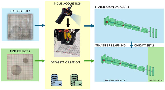
Figure 1.
Flowchart of the transfer learning methodology for acoustic defect classification. Acoustic data from a reference specimen (Test Object 1) trained an initial CNN. This pre-trained model was then fine-tuned via transfer learning using limited data from a second specimen (Test Object 2) with different material characteristics. The adapted model was subsequently evaluated for defect classification on the full Dataset 2, demonstrating improved accuracy and generalization.
In detail, the two test objects were prepared and fixed on an aluminium cube measuring 200 mm on each side, which served as a rigid backing to prevent the movement of the specimens, as shown in Figure 2a. The test objects were designed to include intentional air cavities between the bonded polymeric layers to simulate debonding defects. The materials was chosen for their well-known mechanical characteristics [19]. Test Object 1 is made of poly-methyl-methacrylate (PMMA). Two cavities A and B are modelled by a cylindrical geometry of 50 mm and 25 mm radius and 40 mm height. The plate is 3 mm thick. Test Object 2 shares the same cavity geometry but it is made of poly-vinyl-chloride (PVC) and the plate is 1 mm thick, as shown in the close-up in Figure 2b.
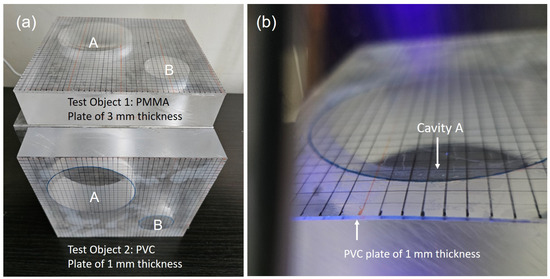
Figure 2.
(a) Photograph of the two test objects mounted on the same aluminium cube (200 mm per side), which serves as a rigid support to constrain vibrations during testing. Test Object 1, located on top, is made of PMMA with a plate thickness of 3 mm. Test Object 2, below, is made of PVC with a plate thickness of 1 mm. Both contain two cylindrical cavities—A (large, 50 mm radius) and B (small, 25 mm radius)—that simulate debonding defects. (b) Close-up view of Cavity A in the PVC specimen, showing the air interface beneath the bonded polymeric layer. The transparency of the material and the surface grid allow visual assessment of defect geometry and position.
Table 1 shows the properties of both materials.

Table 1.
Properties of the PMMA and PVC used for the test objects.
The adhesion between the polymeric layers was achieved using a bisphenol A epoxy resin. The initial acoustic data were acquired using the PICUS system from a reference specimen (Test Object 1). These signals were recorded following controlled mechanical excitation of its surface and stored in audio files that formed the basis of Dataset 1. This dataset was used to train a CNN to classify two predefined defect types embedded in the test object structure.
Once the model was trained on Dataset 1, a transfer learning procedure was applied. Specifically, the pre-trained network was fine-tuned using a limited subset of samples from Dataset 2, which was collected from the second specimen with different material characteristics—primarily in terms of thickness and acoustic response. This step enabled the model to efficiently adapt its internal weights to the new domain with minimal data and computational effort.
Following fine-tuning, the adapted model was evaluated on the full Dataset 2, and the results were used for defect classification across the entire surface. The application of transfer learning led to a notable improvement in classification accuracy, confirming the method’s ability to generalize effectively to new materials.
2.1. System Architecture: PICUS Device
The architecture of the PICUS acquisition system is structured in Figure 3. The system consists of a mechanical actuator, a data acquisition module, and a signal processing unit. The actuator gently taps the surface at predefined locations on a grid, while a microphone captures the resulting acoustic response.
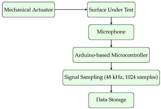
Figure 3.
Schematic diagram of the PICUS system used for non-destructive surface inspection. The system includes a mechanical actuator for stimulus generation, a microphone for acoustic signal capture, and an Arduino-based microcontroller for synchronized control and data acquisition.
The core of the system is an Arduino-based microcontroller that coordinates the timing of the mechanical tap and the acquisition of the audio signal. The signal is sampled at 48 kHz and stored as an array of 1024 samples, corresponding to a short time window that captures the full acoustic impulse response of the stimulated point.
The modular design of PICUS ensures reproducibility, portability, and low cost, making it suitable for scalable applications in surface defect detection. The entire acquisition sequence—from mechanical actuation to audio recording—is fully automated, ensuring consistency and eliminating operator variability.
2.2. Data Acquisition Setup
The acquisition was performed using the PICUS system in a dense grid of 40 × 40 points, resulting in 1600 measurements per dataset. Each measurement captures the acoustic signal generated by the excitation of the PICUS at the specific point, acquired and represented in the time domain for subsequent analysis. Two distinct datasets were created following this protocol, for a total of 3200 individual acquisitions. The test surfaces (Test Object 1 and Test Object 2) used in this study were made of transparent polymeric material, allowing for precise visual identification and annotation of the defect locations. Each acoustic data point was then labelled according to the type of sub-surface defect detected. Specifically, areas identified as non-defective material were assigned Label 0. If a defect was present, such as a cavity between the bonded polymeric layers, where the upper layer could vibrate, the corresponding point was assigned Label 1. This labelling approach, where all defect types (Defect Type 1, Defect Type 2, etc.) are treated equally under Label 1, aims to help the neural network generalize the concept of “defect” as opposed to “non-defect” areas.
Both test object surfaces followed the same labelling scheme. Test Object 1 (Dataset 1) was used to train the neural network, while the second (Dataset 2), with different geometric and acoustic properties (e.g., thickness, material), was used to evaluate the model’s ability to generalize via transfer learning.
2.3. Proposed Neural Network
Given that the dataset comprises one-dimensional time-series data acquired from the PICUS microphone, which captures localized surface excitations, a one-dimensional CNN was adopted. The 1D CNN architecture is particularly well-suited for this application as it can effectively learn and extract temporal patterns and local dependencies within the signal. By applying convolutional filters along the time axis, the network can capture salient features such as transient events and frequency-related characteristics without the need for manual feature engineering. This enables robust characterization of the underlying physical phenomena directly in the time domain, improving the model’s ability to generalize and accurately interpret the measured signals. The proposed CNN is developed using the Keras deep learning library with a TensorFlow backend. The model is implemented using a sequential architecture. The input layer processes a one-dimensional signal of length 1024 with a single channel. The first convolutional block comprises a 1D convolutional layer with 64 filters, a kernel size of 3, and ’same’ padding, and the ReLU (Rectified Linear Unit) activation function is used to introduce non-linearity followed by batch normalization to enhance training stability and convergence. A max pooling operation with a pool size of 2 is then applied to reduce the temporal resolution and computational cost.
The second block increases the model capacity through a convolutional layer with 128 filters, maintaining the same kernel configuration. This is again followed by batch normalization, max pooling with a pool size of 2, and a dropout layer with a dropout rate of 0.3 to prevent overfitting.
A third convolutional block is added to further enhance the feature extraction capability. It consists of a 1D convolutional layer with 256 filters, followed by batch normalization, max pooling, and a dropout layer with an increased dropout rate of 0.5, introducing stronger regularization at deeper layers.
To transition from convolutional to dense layers, a global average pooling (GAP) layer is employed, which reduces the temporal dimension by computing the average over each feature map. The resulting feature vector is fed into two fully connected layers with 128 and 32 units, respectively, each using the ReLU activation function. A dropout layer (rate = 0.5) is applied after the penultimate dense layer to further reduce the risk of overfitting.
The final output layer consists of a fully connected softmax layer, with 2 neurons (equal to the number of output classes), enabling multi-class classification. The network is trained using the Adam optimizer, and categorical cross-entropy is adopted as the loss function. The learning rate , the decay rate of the first-moment , and the decay rate of the second-moment were systematically varied. The optimal performance was achieved with a learning rate of , a first moment decay rate of , and a second moment decay rate of , consistent with the practical recommendations reported in [20,21]. Model performance is evaluated using the classification accuracy metric. The architecture of the proposed neural network is illustrated in Figure 4, which provides a graphical representation of the structure described above.
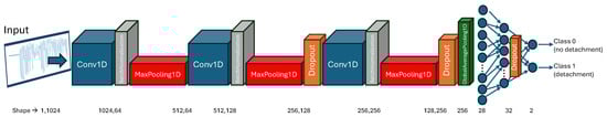
Figure 4.
Schematic representation of the proposed 1D CNN architecture. The model processes a univariate time series of length 1024 and consists of three convolutional layers with ReLU activation, interleaved with max pooling and dropout for feature extraction and regularization. The final classification is performed through fully connected dense layers with a softmax output.
To evaluate the inter-class performance of the proposed model, we employed the classification report provided by the sklearn.metrics.classification_report function [22]. This report summarizes key performance metrics for each individual class, enabling a detailed analysis of the classifier’s ability to distinguish between different target categories. For each class, the classification report computes the following metrics:
Precision: Defined as the ratio between true positives (TP) and the sum of true positives and false negatives (TP + FN), precision measures the accuracy of the positive predictions for each class. High precision indicates a low false positive rate.
Recall (Sensitivity or True Positive Rate): Calculated as the ratio between true positives (TP) and the sum of true positives and false negatives (TP + FN). Recall quantifies the model’s ability to correctly identify all relevant instances of a given class.
F1-Score: The harmonic mean of precision and recall, providing a balanced measure that accounts for both false positives and false negatives. This metric is particularly useful when dealing with class imbalance.
Support: The number of true instances for each class in the test dataset, indicating the distribution of samples across classes.
In addition to per-class metrics, the report also includes macro, micro, and weighted averages of precision, recall, and F1-score, offering a global view of the classifier’s performance that takes into account either all classes equally (macro), the individual decisions (micro), or the class frequency (weighted).
2.4. Transfer Learning
Transfer learning is a machine learning technique in which knowledge gained while solving one problem (the source task) is leveraged to improve learning performance in a different but related problem (the target task). This can be formally defined through the concepts of domain and task.
A domain is defined as
where denotes the feature space, and is the marginal probability distribution of data .
Given a domain , a task is defined as
where is the label space, and is the predictive function to be learned.
In the context of transfer learning, we define
- A source domain with an associated source task.
- A target domain with a corresponding target task.
Transfer learning aims to improve the performance of the predictive function in the target domain , by leveraging knowledge from and [23], even when
In deep learning applications, transfer learning typically involves reusing the parameters learned from a source model and adapting them to a target model:
where represents the parameter updates obtained through fine-tuning on the target dataset.
In this study, we adopted a fine-tuning strategy within a transfer learning framework to adapt a pre-trained model to a second, distinct dataset. This approach enables the transfer of knowledge extracted from one or more source tasks to a new learning scenario, thereby enhancing generalization capabilities and reducing the amount of labelled data required for training in the target domain [23].
Transfer learning, therefore, allows for differences in domains, tasks, and data distributions between training and testing stages, providing a flexible and efficient solution in scenarios where labelled data in the target domain is scarce or expensive to obtain.
Based on the relationship between source and target domains and tasks, transfer learning can be categorized into
- Inductive transfer learning: the target task is supervised (i.e., labelled data is available).
- Transductive transfer learning (domain adaptation): the source and target tasks are the same, but the domains differ.
- Unsupervised transfer learning: neither source nor target tasks have labelled data, focusing primarily on representation learning.
This formalism provides a theoretical foundation for the development and assessment of transfer learning techniques across various application domains. This study leverages a CNN in combination with transfer learning to improve performance on a target task characterized by limited annotated data. Transfer learning in a CNN refers to the reuse of a neural network model trained on a source task to facilitate learning in a different but related target task. This is particularly effective when the source task has access to large-scale labelled data, while the target task suffers from limited annotated samples.
A CNN model trained on the source task learns a set of parameters:
where represents the weights of the ℓ-th layer of the CNN with L total layers.
In transfer learning, the target model reuses the parameters of the first layers of the source model:
The remaining layers, , are either
- Re-initialized and trained from scratch (partial transfer).
- Fine-tuned based on the target data (full fine-tuning).
The final target model parameters are
with the following:
where denotes the parameter updates derived from fine-tuning on the target dataset.
This formulation allows the CNN to retain general low-level features (e.g., edges, textures) learned from the source task while adapting high-level semantic representations to the target task. The optimization objective in the target domain becomes
where is the loss function for the target task (e.g., cross-entropy), and are the target data and labels.
Transfer learning via CNN is particularly beneficial when but the feature spaces are sufficiently similar to allow knowledge reuse.
This is typically achieved by transferring learned features, model parameters, or data representations from the source to the target. Therefore, this can be considered a paradigm within machine learning where a model, meticulously pre-trained on an extensive dataset for a generalized source task, is subsequently adapted or “transferred” to a distinct yet inherently related target task. This methodology fundamentally deviates from training a model ab initio, which necessitates prodigious volumes of labelled data and computational expenditure. The underlying principle is the leveraging of knowledge encapsulation within the pre-trained model, specifically its learned hierarchical feature representations and optimized parametric values (weights and biases), to expedite and enhance learning on the target task, particularly when target-specific labelled data is scarce. The technical mechanisms of knowledge transfer unfold in a gradient-driven fashion. A pre-trained deep neural network, often a CNN for computer vision or a Transformer-based architecture for Natural Language Processing (NLP), serves as the foundational architecture. These models, having been exposed to vast and diverse datasets, develop robust internal representations. Early layers of such networks tend to learn universal, low-level features—such as edge detectors, gradient orientations, or basic n-gram patterns—which are largely invariant to the specific downstream task. Deeper layers progressively synthesize these low-level features into more abstract and semantically rich representations, ultimately becoming more task-specific. In feature extraction, the base or convolutional embedding layers of the pre-trained model, which are responsible for extracting salient features, are treated as fixed and untrainable components. Their learned weights are “frozen,” meaning they are not updated during backpropagation to the new target dataset. The output of these frozen layers, essentially a high-dimensional feature vector, then serves as input to a newly added, task-specific “head” (e.g., a fully connected classifier) that is randomly initialized and trained from scratch on the target data. This method is computationally efficient, as only newly added layers require gradient computation and weight updates, effectively using the pre-trained model as a powerful general-purpose feature extractor [24].
Fine-tuning, a more sophisticated form of transfer learning, involves not only adding new task-specific layers but also selectively unfreezing and continuing to train some or all of the pre-trained layers on the target dataset. A specialized variant of transfer learning, domain adaptation, addresses scenarios where the source and target tasks may be identical, but there is a significant statistical disparity, or “domain shift,” between their respective data distributions. The effectiveness of transfer learning stems from the empirically observed phenomenon that deep neural networks learn hierarchical representations, where lower layers capture generalizable patterns and higher layers capture more abstract, task-specific features. By transferring these robust initial layers, the model benefits from a strong inductive bias, requiring less data and fewer training iterations to achieve high performance on new, related tasks. This makes transfer learning an indispensable technique for tasks with limited labelled data or when computational resources are limited.
This approach is particularly advantageous in our case as the domain adaptation is applicable in the two datasets and is shown schematically in Figure 5, which shows how the model exploits the features and patterns learned during the initial training.
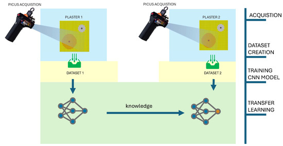
Figure 5.
Schematic representation of knowledge transfer from Test Object 1 to Test Object 2 through the application of transfer learning.
Specifically, for this adaptation, we employed a feature extraction strategy by freezing the weights of all layers except for the final two in the pre-existing model. This allows the network to retain previously learned representations while adapting to the new domain through the fine-tuning of its final layers. The line for layer in model.layers[:−3]: layer.trainable = False achieves this by setting the trainable attribute to False for every layer except for the last three (two dense layers and dropout in our case). By freezing these earlier layers, we essentially preserve the low-level and high-level feature detectors that the model has already learned. Only the weights of the final dense layers are allowed to be updated during training on the new dataset. This targeted fine-tuning allows the model to learn the specific mappings from the pre-extracted features to the new target classes, without risking the degradation of the robust feature representations learned from the original, larger dataset. This method typically leads to faster convergence and improved performance on the new task compared to training a model from scratch. The procedure is graphically illustrated in Figure 6, where the frozen weights and the fine-tuned part of the network are highlighted using different colours.
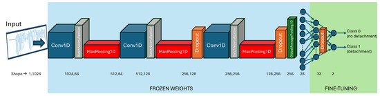
Figure 6.
Visual representation of the transfer learning strategy: frozen layers are marked in blue, while the trainable layers adapted to the new task are highlighted in green.
3. Results
This section presents the results obtained from the two samples processed using the proposed neural network models. In particular, the outcomes illustrate three distinct types of analysis that can be summarized as the generalization tests, transfer learning, and training without prior knowledge, i.e., initialized network.
In the first experimental phase, a one-dimensional 1D-CNN was trained using the data acquired from Test Object 1 to perform a defect classification with training on a portion of the surface dataset and testing on the remaining portion of the dataset. The dataset was randomly split into a training set (80%) and a test set (20%), allowing the network to learn how to classify defective and non-defective regions. The results indicate that the model achieved a good level of precision in distinguishing between these two classes as shown in the classification report proposed in Table 2.
Table 2.
Model classification report performed on Test Object 1.
In the second phase, we evaluated the generalization capability of the trained network. Specifically, the model trained exclusively on Test Object 1 was tested on an entirely new object (Test Object 2), to assess its ability to classify previously unseen data. This step is particularly significant, as it simulates a change in context. Despite differences in surface geometry and structure, the network maintained strong classification performance. As shown in Table 3, the model achieved a class 1 precision of 88%, indicating that it was able to correctly identify defective areas even under substantially different conditions. These results confirm that the model generalized well, responding correctly to changes in the physical characteristics of the input data.
Table 3.
Classification report of the model trained on Test Object 1 and tested in Test Object 2.
To achieve enhanced performance and ensure the network’s adaptability to unseen data, we employed a transfer learning methodology. Our approach involved fine-tuning the terminal three layers of the neural network: the two fully connected layers and the dropout layer that comprises the classifier block. This fine-tuning utilized a concentrated subset of data from Test Object 2, specifically 160 samples, representing 10% of its total. Throughout this phase, the weights of the network’s foundational layers were intentionally frozen. Although the model demonstrated robust precision in previous evaluations, the application of transfer learning allowed for a more granular optimization of its parameters, leading to superior defect classification accuracy as reported in Table 4. This consequently augmented the system’s responsiveness to subtle defective regions, a critical advantage when facing dynamic operational environments.
Table 4.
Classification report showing precision, recall, F1-score, and support for each class. The model was initially trained on Test Object 1 using a transfer learning approach and subsequently fine-tuned for Test Object 2.
To validate the effectiveness of transfer learning, an additional control experiment was performed. A randomly initialized network (with no prior training) was tested directly on the Test Object 2 dataset used for transfer learning. As reported in Table 5, the model failed to classify the defective regions, confirming that the small data subset alone is not sufficient to train a model from scratch for this task. This result reinforces the necessity of a well-structured and representative dataset to ensure adequate model performance.
Table 5.
Classification report showing precision, recall, F1-score, and support for each class. The model was trained on Test Object 1 using a transfer learning approach and evaluated on Test Object 2 without additional fine-tuning.
Finally, to qualitatively assess the model’s prediction capabilities, a defect map of Test Object 2 is provided in Figure 7. The output was generated by applying the network—trained on Test Object 1 to the entire dataset of Test Object 2. As seen in the resulting image, the defective regions are correctly highlighted and well-localized, demonstrating the effectiveness of the model in visualizing defects based on previously unseen input.
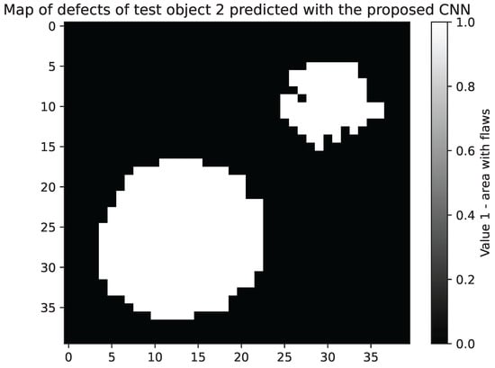
Figure 7.
Defect localization map for Test Object 2, obtained by applying a CNN model trained on Test Object 1.
4. Discussion
This research investigated how transfer learning, integrated with a 1D-CNN classifier, can enhance non-destructive material testing. We particularly focused on overcoming the pervasive and challenging issue of surface variability. The study’s results affirm that our developed model exhibits strong generalization capabilities across varying acquisition surfaces. This crucial characteristic ensures its practical viability in applications where surface uniformity is frequently unpredictable.
Therefore, this research specifically addressed the pervasive and challenging issue of variability in surface properties. The findings unequivocally prove the proposed model’s ability to generalize robustly across diverse acquisition conditions. This represents a pivotal advance, as such adaptability is paramount for reliable deployment in real-world scenarios where consistent surface conditions are often unattainable. Our experimental setup involved training the network on a first specimen (Test Object 1) and then rigorously evaluating its performance on a second (Test Object 2), with highly encouraging outcomes. Notably, the classification performance, particularly precision, achieved improvements, which is crucial for a field demanding highly accurate defect identification.
This study represents a first step toward the deployment of a field-capable device that can locally fine-tune a neural network through transfer learning, enabling widespread monitoring of potential defects in various types of materials, including in the restoration sector or in the structural and materials health sector.
The proposed approach highlights the potential of integrating the PICUS device as a core component in a highly adaptable, easy-to-use tool. This system can leverage experimental lab data to adapt neural network parameters in response to new environmental or material conditions.
One of the central challenges for NDT analysis is the identification of different defect-prone zones, such as detachments or hollow areas, often based on limited prior knowledge. Here, AI offers a viable and scalable solution. The proposed workflow allows training to begin in the lab using test objects with known defects, facilitating a supervised learning setup. By registering coordinates during acquisition, labels can be accurately assigned, which supports effective and precise training.
While this approach requires an initial data acquisition effort, it brings significant advantages during the fine-tuning phase, where the network is adapted to specific surfaces encountered in the various areas of employment. Importantly, through transfer learning, the network can be retrained using only a small subset of annotated data, reducing the burden on the expert, who would otherwise need to manually label large datasets to train a model from scratch.
This methodology presents clear benefits in terms of efficiency and scalability and significantly accelerates the deployment of trained models during diagnosis projects. In our view, this approach represents a promising and novel application of transfer learning in the SHM (Structural Health Monitoring) application, especially considering that most of the existing literature focuses on domains such as medicine or acoustic diagnostics.
As shown in our results, the model’s performance is in line with expectations and confirms the suitability of this type of neural architecture for identifying defects in complex, variable surfaces.
5. Conclusions
In this study, we presented an approach that combines low-cost acoustic signal acquisition via the PICUS device with deep learning and transfer learning techniques to enable scalable and accurate non-destructive defect detection. By training a CNN on a reference surface and adapting it to a second surface through transfer learning, we achieved a significant improvement in classification accuracy—from an initial 88% to 95% on the target dataset. This confirms the effectiveness of transfer learning to effectively adapt to different acoustic domains with a minimum amount of data.
The proposed method is particularly effective for bonded polymeric structures, and it proves to be particularly suitable for real-world scenarios where variability in material properties is common and large-scale data acquisition may be impractical. With this approach, a small number of samples from a new surface can suffice to enable a complete and detailed defect mapping, making the system highly efficient and accessible for on-field applications.
Although the current model demonstrates promising results in generating defect maps consistent with the test object, its interpretability remains limited. Explainability techniques, such as saliency maps and activation analysis, represent a valuable avenue for future research to better understand the discriminative signal features and improve the model’s reliability. Additionally, deeper insight into the correlation between specific acoustic signatures and defect types will allow for further optimization of classification accuracy. Future work will focus on integrating these explainability methods and refining the model architecture and feature extraction strategies accordingly.
Future developments will also focus on extending the methodology to different materials and more complex defect patterns, broadening the applicability of the system. Additionally, enhanced neural network models tailored to acoustic signal features could further improve the precision and robustness of defect identification, paving the way toward fully autonomous and explainable NDE systems.
Author Contributions
Conceptualization, M.L.G., F.M., G.C. and A.S.; methodology, M.L.G., F.M. and G.C.; software, M.L.G. and F.M.; validation, M.L.G., F.M. and G.C.; formal analysis, M.L.G., F.M., G.C. and A.S.; investigation, M.L.G., F.M. and G.C.; resources, M.L.G., F.M., G.C. and A.S.; data curation, M.L.G., F.M. and G.C.; writing—original draft preparation, M.L.G. and F.M.; writing—review and editing, M.L.G., F.M. and G.C.; visualization, M.L.G. and F.M.; supervision, G.C. and A.S.; project administration, G.C. and A.S. All authors have read and agreed to the published version of the manuscript.
Funding
This research received no external funding.
Institutional Review Board Statement
Not applicable.
Informed Consent Statement
Not applicable.
Data Availability Statement
The data presented in this study are available on request from the corresponding author.
Conflicts of Interest
The authors declare no conflicts of interest.
References
- Gupta, M.; Khan, M.A.; Butola, R.; Singari, R.M. Advances in applications of Non-Destructive Testing (NDT): A review. Adv. Mater. Process. Technol. 2022, 8, 2286–2307. [Google Scholar] [CrossRef]
- Gholizadeh, S. A review of non-destructive testing methods of composite materials. Procedia Struct. Integr. 2016, 1, 50–57. [Google Scholar] [CrossRef]
- Kosel, F.; Petrišič, J.; Kuselj, B.; Kosel, T.; Šajn, V.; Brojan, M. Local buckling and debonding problem of a bonded two-layer plate. Arch. Appl. Mech. 2005, 74, 704–726. [Google Scholar] [CrossRef]
- Lago, S.; Brignolo, S.; Cuccaro, R.; Musacchio, C.; Giuliano Albo, P.; Tarizzo, P. Application of acoustic methods for a non-destructive evaluation of the elastic properties of several typologies of materials. Appl. Acoust. 2014, 75, 10–16. [Google Scholar] [CrossRef]
- Wang, B.; Zhong, S.; Lee, T.L.; Fancey, K.S.; Mi, J. Non-destructive testing and evaluation of composite materials/structures: A state-of-the-art review. Adv. Mech. Eng. 2020, 12, 1687814020913761. [Google Scholar] [CrossRef]
- Wang, X.; Wang, J.; Huang, Z.; Li, X. Measurement Interface Stiffness of Bonded Structures Using Air-Coupled Ultrasonic Transmission Technology. IEEE Access 2021, 9, 43494–43503. [Google Scholar] [CrossRef]
- Melchiorre, J.; D’Amato, L.; Agostini, F.; Manuello, A. Deep-Learning-Based Onset Time Precision in Acoustic Emission Non-Destructive Testing. In Proceedings of the 2024 IEEE International Workshop on Metrology for Living Environment (MetroLivEnv), Chania, Greece, 12–14 June 2024; pp. 367–372. [Google Scholar] [CrossRef]
- Hassani, S.; Dackermann, U. A Systematic Review of Advanced Sensor Technologies for Non-Destructive Testing and Structural Health Monitoring. Sensors 2023, 23, 2204. [Google Scholar] [CrossRef] [PubMed]
- Sarkar, D.; Bali, R.; Ghosh, T. Hands-On Transfer Learning with Python: Implement Advanced Deep Learning and Neural Network Models Using TensorFlow and Keras; Packt Publishing Ltd.: Birmingham, UK, 2018. [Google Scholar]
- Kim, H.E.; Cosa-Linan, A.; Santhanam, N.; Jannesari, M.; Maros, M.E.; Ganslandt, T. Transfer learning for medical image classification: A literature review. BMC Med. Imaging 2022, 22, 69. [Google Scholar] [CrossRef] [PubMed]
- Salehi, A.W.; Khan, S.; Gupta, G.; Alabduallah, B.I.; Almjally, A.; Alsolai, H.; Siddiqui, T.; Mellit, A. A study of CNN and transfer learning in medical imaging: Advantages, challenges, future scope. Sustainability 2023, 15, 5930. [Google Scholar] [CrossRef]
- Li, C.; Zhang, S.; Qin, Y.; Estupinan, E. A systematic review of deep transfer learning for machinery fault diagnosis. Neurocomputing 2020, 407, 121–135. [Google Scholar] [CrossRef]
- Chen, H.; Luo, H.; Huang, B.; Jiang, B.; Kaynak, O. Transfer learning-motivated intelligent fault diagnosis designs: A survey, insights, and perspectives. IEEE Trans. Neural Netw. Learn. Syst. 2023, 35, 2969–2983. [Google Scholar] [CrossRef] [PubMed]
- Pan, Q.; Bao, Y.; Li, H. Transfer learning-based data anomaly detection for structural health monitoring. Struct. Health Monit. 2023, 22, 3077–3091. [Google Scholar] [CrossRef]
- Azad, M.M.; Kim, S.; Cheon, Y.B.; Kim, H.S. Intelligent structural health monitoring of composite structures using machine learning, deep learning, and transfer learning: A review. Adv. Compos. Mater. 2024, 33, 162–188. [Google Scholar] [CrossRef]
- Giudice, M.L.; Mariani, F.; Caliano, G.; Salvini, A. Deep learning for the detection and classification of adhesion defects in antique plaster layers. J. Cult. Herit. 2024, 69, 78–85. [Google Scholar] [CrossRef]
- Caliano, G.; Mariani, F.; Salvini, A. A portable and autonomous system for the diagnosis of the structural health of cultural heritage (PICUS). In Proceedings of the 2023 IMEKO TC-4 International Conference on Metrology for Archaeology and Cultural Heritage, Rome, Italy, 19–21 October 2023. [Google Scholar]
- Cawley, P.; Adams, R.D. The mechanics of the coin-tap method of non-destructive testing. J. Sound Vib. 1988, 122, 299–316. [Google Scholar] [CrossRef]
- Ashby, M. Material Property Data for Engineering Materials, 5th ed.; Compiled by Ashby, M.; Part of a Set of Teaching Resources; Department of Engineering, University of Cambridge: Cambridge, UK, 2021. [Google Scholar]
- Kingma, D.P.; Ba, J. Adam: A method for stochastic optimization. arXiv 2014, arXiv:1412.6980. [Google Scholar]
- Bengio, Y. Practical recommendations for gradient-based training of deep architectures. In Neural Networks: Tricks of the Trade, 2nd ed.; Springer: Berlin/Heidelberg, Germany, 2012; pp. 437–478. [Google Scholar]
- Scikit-Learn Developers. Sklearn.Metrics.Classification_Report. 2024. Available online: https://scikit-learn.org/stable/modules/generated/sklearn.metrics.classification_report.html (accessed on 21 May 2025).
- Pan, S.J.; Yang, Q. A Survey on Transfer Learning. IEEE Trans. Knowl. Data Eng. 2010, 22, 1345–1359. [Google Scholar] [CrossRef]
- Weiss, K.; Khoshgoftaar, T.M.; Wang, D. A survey of transfer learning. J. Big Data 2016, 3, 9. [Google Scholar] [CrossRef]
Disclaimer/Publisher’s Note: The statements, opinions and data contained in all publications are solely those of the individual author(s) and contributor(s) and not of MDPI and/or the editor(s). MDPI and/or the editor(s) disclaim responsibility for any injury to people or property resulting from any ideas, methods, instructions or products referred to in the content. |
© 2025 by the authors. Licensee MDPI, Basel, Switzerland. This article is an open access article distributed under the terms and conditions of the Creative Commons Attribution (CC BY) license (https://creativecommons.org/licenses/by/4.0/).