Enhanced Pilot Attention Monitoring: A Time-Frequency EEG Analysis Using CNN–LSTM Networks for Aviation Safety

Abstract

Despite significant technological advancements in aviation safety systems, human-operator condition monitoring remains a critical challenge, with more than 75% of aircraft incidents stemming from attention-related perceptual failures. This study addresses a fundamental question in sensor-based condition monitoring: how can temporal- and frequency-domain EEG sensor data be optimally integrated to detect precursors of system failure in human–machine interfaces? We propose a three-stage diagnostic framework that mirrors industrial condition monitoring approaches. First, raw EEG sensor signals undergo preprocessing into standardized one-second epochs. Second, a novel hybrid feature-extraction methodology combines time- and frequency-domain features to create comprehensive sensor signatures of neural states. Finally, our dual-architecture CNN–LSTM model processes spatial patterns via CNNs while capturing temporal degradation signals via LSTMs, enabling robust classification in noisy operational environments. Our contributions include (1) a multimodal data fusion approach for EEG sensors that provides a more comprehensive representation of operator conditions, and (2) an artificial intelligence architecture that balances spatial and temporal analysis for the predictive maintenance of attention states. When validated on aviation-related EEG datasets, our condition monitoring system achieved significantly higher diagnostic accuracy across various noise conditions compared to existing approaches. The practical applications extend beyond theoretical improvement, offering a pathway to implement more reliable human–machine interface monitoring in critical systems, potentially preventing catastrophic failures by detecting condition anomalies before they propagate through the system.

1. Introduction

Aviation safety has made tremendous strides through technological advancements, yet the human element remains a crucial vulnerability in the cockpit. The striking statistic that more than 75% of pilot errors stem from perceptual failures [1] reveals an uncomfortable truth: even highly trained professionals can experience dangerous lapses in attention. These lapses do not occur randomly but fall into distinct patterns that have been identified through a careful analysis of incident data.

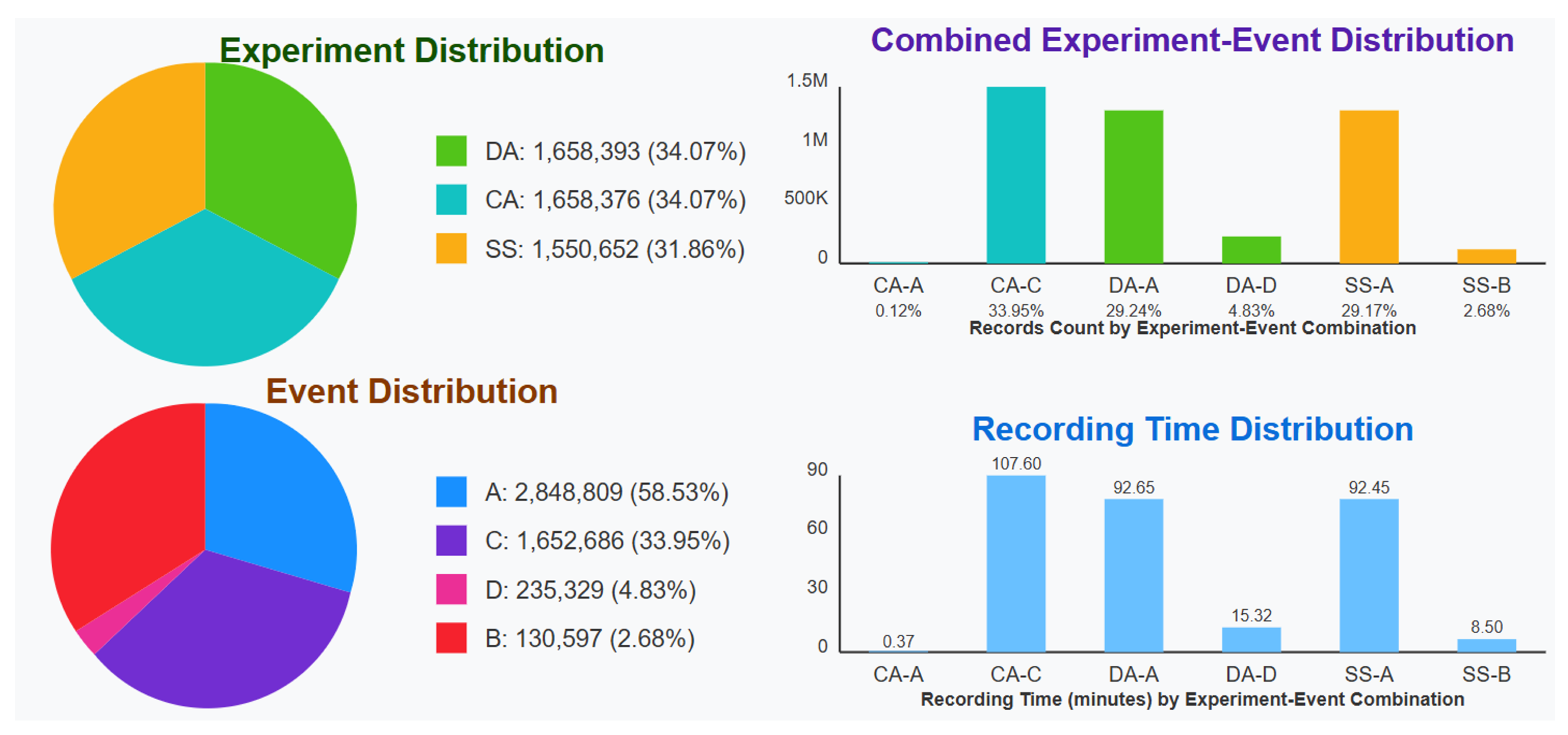
According to data analyzed by the International Air Transport Association (IATA), there were 45 plane crashes caused by pilots losing control of the aircraft, resulting in 1645 fatalities between 2012 and 2021 [2,3]. More alarmingly, when examining the 18 aircraft accidents investigated by the Commercial Aviation Safety Team (CAST), the discovery that attention deficiencies were involved in 16 of these incidents [4] pointed researchers toward three specific attention-related pilot performance deficiencies (APPD) that demanded deeper investigation.

Channelized attention (CA) represents a particularly insidious threat, as pilots become fixated on a single task or instrument while neglecting other critical flight information. Diverted attention (DA) emerges when pilots attempt to process too many competing tasks simultaneously, resulting in the incomplete processing of flight-critical information. Perhaps most dangerous is the startle/surprise (SS) state, which produces a cognitive paralysis during critical moments when immediate action is required. Together, these three states—CA, DA, and SS—represent the most dangerous attention-related conditions that precede loss of aircraft control [5,6,7].

The identification of these three distinct attention states created a compelling research question: could these states be detected before they lead to dangerous situations? This is where electroencephalography (EEG) enters the picture as a promising solution. EEG offers unique capabilities to detect transient alterations in brain activity that may indicate attention deficits before they manifest as observable behavior. By monitoring brain activity patterns, researchers hope to identify the neural signatures of CA, DA, and SS states as they emerge, potentially enabling interventions before critical errors occur. However, the path forward is not simple—EEG signals are notorious for collecting artifacts from environmental factors and physiological phenomena, creating significant challenges for developing reliable machine learning models [8,9].

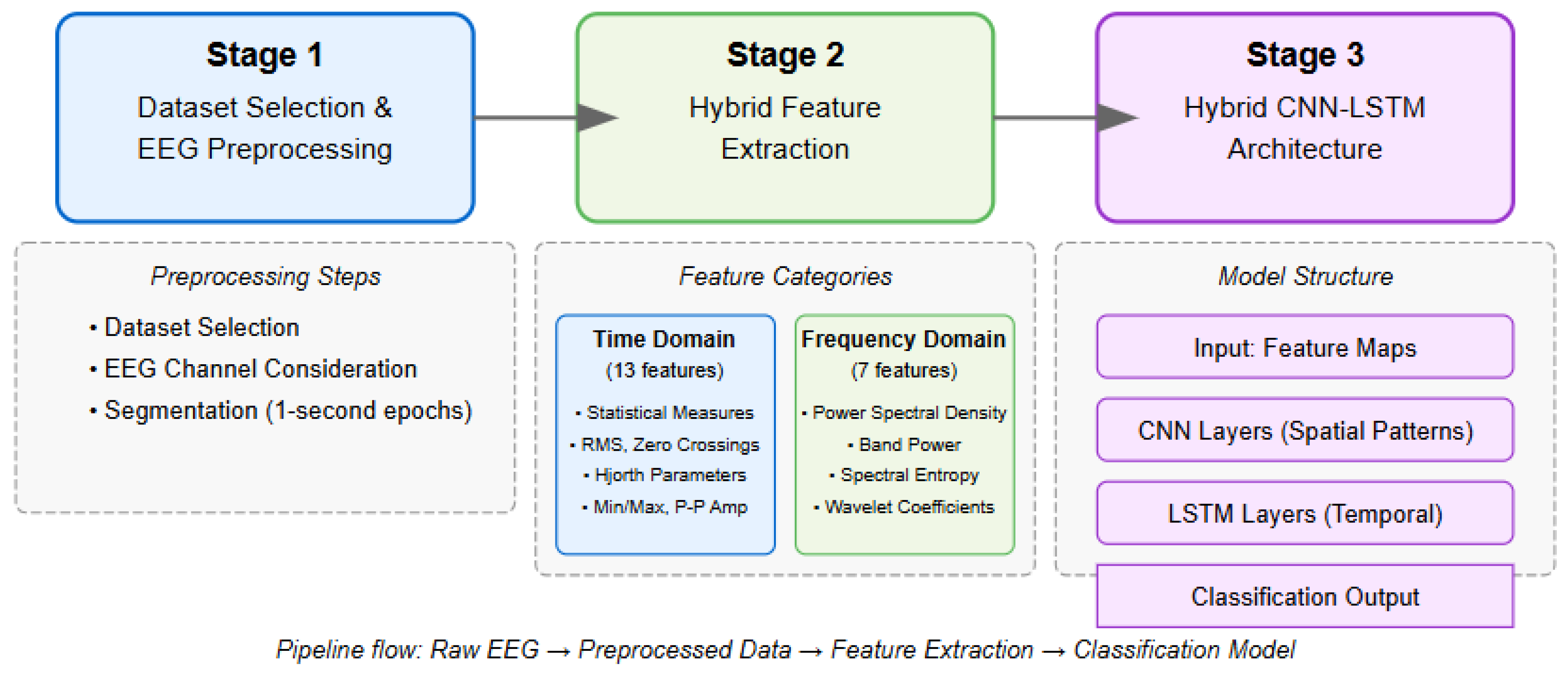
To address these limitations, we propose a hybrid feature model combined with a CNN–LSTM architecture for the multiclass classification of all critical pilot mental states. Our approach deliberately combines manually extracted temporal- and frequency-domain features with the pattern recognition capabilities of deep learning, leveraging complementary information. The learning occurs in two stages: first through our carefully engineered feature pool that explicitly captures known EEG characteristics, and then through a hybrid CNN–LSTM architecture that identifies higher-level patterns from these features.

Our comprehensive three-stage approach begins with meticulous dataset selection and preprocessing, where raw EEG signals are prepared and segmented into one-second epochs to capture complete neurophysiological events while ensuring sufficient frequency resolution. The second stage extracts a hybrid feature pool, combining 13 time-domain features (such as statistical moments, RMS, and Hjorth parameters) with 7 frequency-domain features (including spectral power, entropy, and wavelet coefficients) to fully characterize both temporal dynamics and spectral properties of brain activity. The final stage implements our hybrid CNN–LSTM architecture, which combines the strengths of two complementary neural network approaches. The CNN component excels at detecting local spatial patterns within the feature maps, functioning as a hierarchical feature detector that can identify key discriminative patterns while being relatively invariant to their exact position in the input. Meanwhile, the LSTM component addresses the critical temporal dimension of EEG data, modeling sequential dependencies and capturing how patterns of brain activity evolve over time—a crucial aspect for distinguishing between different attention states that may share similar instantaneous characteristics but differ in their temporal dynamics.

The primary contributions of this research are as follows:

• The development of a novel hybrid feature-extraction approach that combines complementary temporal- and frequency-domain features, creating a comprehensive representation of EEG signals that captures the complex neural signatures of critical pilot attention states (CA, DA, and SS);
• The design and implementation of a specialized CNN–LSTM architecture that leverages the strengths of both convolutional neural networks for spatial pattern recognition and long short-term memory networks for temporal dependency modeling, resulting in superior classification performance, even in the presence of noise and artifacts that are typical in real-world aviation environments.

Our proposed approach is validated using a publicly available dataset from Kaggle, released under the name ‘Reducing Commercial Aviation Fatalities’ [10]. We have rigorously analyzed the capabilities of our proposed approach under various noisy and robust conditions and compared it extensively with various state-of-the-art approaches. Our method exhibits superior performance.

2. Related Works

The monitoring of pilot mental states and workload has emerged as a critical research area in aviation safety, with various approaches being developed to detect attention deficits and cognitive impairments before they lead to critical incidents. This comprehensive review examines existing methodologies, ranging from EEG-based approaches to alternative sensing modalities, highlighting their contributions, limitations, and relative standing in the field.

The EEG-based analysis of pilot mental states has evolved significantly from conventional preprocessing to sophisticated automated approaches. Traditional techniques included filtering methodologies, as demonstrated by Roza et al. [11], who used a band-pass filter at 12–30 Hz to isolate beta rhythm activity, and Han et al. [12], who implemented filtering at 0.1–50 Hz before applying Independent Component Analysis (ICA). Despite their widespread adoption, these methods showed inherent limitations, with Alreshidi et al. [13] finding no significant performance improvement when comparing filtered data to ICA-processed data. This recognition led to the emergence of automated preprocessing methods, with Autoreject [14] being particularly notable for its ability to automatically identify and repair erroneous EEG segments using Bayesian hyperparameter optimization and cross-validation, as successfully implemented by Bonassi et al. [15] and Pousson et al. [16]. These advances in preprocessing have focused on improving signal quality while preserving critical neurophysiological information, addressing the inherent challenges of artifact contamination in real-world aviation environments.

Feature-extraction techniques have undergone substantial evolution from basic statistical features [17,18] to sophisticated approaches targeting specific frequency bands and their neurophysiological correlates. Wu et al. [19] employed the power spectrum curve area representation of decomposed brain waves through wavelet packet transform, while Binias et al. [20] extracted logarithmic band-power features using common spatial pattern filtering. Recent research has particularly emphasized the importance of beta-wave activity in pilot workload assessment. Li et al. [21] conducted a comprehensive investigation of EEG characteristics during turning phases, focusing specifically on the energy ratio of beta waves and Shannon entropy. Their findings revealed significant changes in beta wave energy and Shannon entropy during left and right turns compared to cruising phases, with psychological workload demonstrably increasing during these critical flight maneuvers. The study achieved an impressive classification accuracy of 98.92% for training and 93.67% for testing using support vector machines, establishing beta-wave analysis as a reliable indicator of pilot cognitive state changes.

Building upon this foundation, Feng et al. [22] further explored the sensitivity of beta-wave sub-bands, specifically 16–20 Hz, 20–24 Hz, and 24–30 Hz, for situation awareness classification. Their comprehensive analysis of 48 participants revealed that relative power in these beta sub-bands was significantly higher in high-situation-awareness groups compared to low-situation-awareness groups across central, central–parietal, and parietal brain regions. Using general supervised machine learning classifiers, they achieved classification accuracies exceeding 75%, with logistic regression and decision trees reaching 92% accuracy while maintaining good interpretability, demonstrating the practical viability of beta-wave-based cognitive state assessment.

The advancement toward more sophisticated mathematical frameworks has been exemplified by Riemannian geometry-based methods, which have gained considerable traction in recent years. Researchers [23] demonstrated how covariance matrices could be represented as vectors in the tangent space of the Riemannian manifold, providing a novel mathematical framework for EEG analysis that addresses some of the limitations of traditional Euclidean-based approaches. Majidov and Whangbo [24] built upon this foundation by computing covariance matrices obtained through spatial filtering and mapping them onto the tangent space, offering improved robustness to inter-subject variability and enhanced generalization across different pilot populations.

Classification methodologies have evolved from traditional machine learning to advanced deep learning architectures, reflecting the field’s growing recognition of the complexity inherent in pilot cognitive state assessment. Johnson et al. [25] investigated six classification algorithms for categorizing task complexity, including naïve Bayes, decision trees, and support vector machines, establishing baseline performance metrics for comparative analysis. Han et al. [12] proposed a more sophisticated detection system using a multimodal deep learning network with CNN and LSTM components to detect pilot mental states, including distraction, workload, fatigue, and normal states, demonstrating the potential of hybrid architectures for capturing both spatial and temporal patterns in neural data. Wu et al. [19] presented a deep contractive autoencoder for identifying mental fatigue with up to 91.67% accuracy, while, for Attention-related Pilot Performance Decrements (APPD), Harrivel et al. [26] employed random forest, extreme gradient boosting, and deep neural networks to predict continuous attention, diverted attention, and low-workload states in flight simulators.

While EEG-based approaches have shown considerable promise, alternative sensing modalities have been explored for pilot monitoring, each offering distinct advantages and limitations that complement neural-based measurements. Eye-tracking technology represents a particularly compelling alternative, providing non-invasive monitoring of visual attention patterns and cognitive workload indicators with high temporal resolution. Cheng et al. [27] demonstrated the effectiveness of eye-tracking for pilot workload assessment during helicopter autorotative gliding, revealing significant changes in fixation patterns with shorter fixation durations but greater fixation numbers during critical flight phases. Their study showed that mean pupil diameter exhibited larger variations during autorotative glide (mean: 5.326 mm, standard deviation: 0.126 mm) compared to level flight (mean: 5.229 mm, standard deviation: 0.059 mm), indicating increased cognitive workload. The pilots allocated 81% of their attention to critical instruments including tachometer, airspeed indicator, and forward views, shifting from low-frequency long gaze patterns during normal flight to high-frequency short gaze patterns during emergency procedures, demonstrating the utility of eye-tracking for real-time workload assessment.

Facial recognition systems have emerged as another viable approach for detecting fatigue and drowsiness, offering contactless monitoring that can be integrated with existing cockpit camera systems. Samy et al. [28] developed a real-time facial recognition system using a histogram of oriented gradients (HOG) and support vector machines (SVMs) for drowsiness detection, achieving 96.8% accuracy in ideal conditions. Their approach demonstrated resilience to facial occlusions and categorized driver states into tired, dynamic, and resting conditions using 68 facial landmark detectors, with the system continuously monitoring subtle changes in facial expressions such as slow eye blinks and changes in head position as early indicators of fatigue.

The comparative analysis of these sensing modalities reveals distinct advantages and limitations that influence their suitability for aviation applications. EEG-based approaches provide a direct measurement of neural activity and can detect cognitive state changes before behavioral manifestations, offering the most sensitive indication of mental state transitions. However, they are susceptible to motion artifacts, require specialized electrode placement, and may be impractical for routine flight operations due to setup complexity and potential interference with standard pilot equipment. Eye-tracking systems offer non-invasive monitoring with high temporal resolution and direct correlation with visual attention patterns, operating continuously without interfering with pilot activities, though they may be affected by lighting conditions, head movements, and calibration requirements. Facial recognition approaches provide contactless monitoring, suitable for existing cockpit infrastructure, and can detect multiple fatigue indicators simultaneously, but may be limited by environmental factors such as lighting conditions, facial occlusions, and individual variations in facial expressions.

Despite these significant advancements, existing approaches exhibit substantial shortcomings that limit their practical application in aviation settings. Current EEG-based methods predominantly rely on manual preprocessing techniques, which introduce inconsistency across studies and require substantial domain expertise to implement effectively. Many frameworks focus narrowly on binary classification tasks such as fatigued versus non-fatigued states, failing to address the complex, multiclass nature of pilot mental states that occur during actual flight operations. Furthermore, most approaches suffer from an inability to simultaneously capture both temporal dynamics and spatial patterns in EEG signals, which represents a critical requirement for understanding the rapidly changing mental states experienced by pilots during different phases of flight. The majority of existing studies target only subset combinations of mental states rather than comprehensively addressing all relevant Attention-related Pilot Performance Decrement (APPD) states alongside normal operating conditions using EEG data alone. While Alrashidi et al. [29] attempted to bridge some of these gaps through automated preprocessing and ensemble learning, their approach still faces challenges in real-time implementation, computational efficiency, and capturing the full spectrum of temporal–spatial relationships inherent in EEG signals. Their use of Riemannian geometry features—a mathematical framework that treats EEG covariance matrices as points on a curved manifold rather than in traditional Euclidean space—offers theoretical advantages for representing the complex statistical relationships between brain regions. However, this approach requires computationally expensive operations such as matrix logarithms and geodesic distance calculations, which can limit practical deployment in time-sensitive applications. Moreover, while Riemannian features excel at capturing spatial correlations between electrodes, they may not fully preserve the rapid temporal dynamics that characterize attention state transitions in pilot monitoring scenarios.

Additional limitations include substantial restrictions in generalizability across different pilots and flight scenarios, with many techniques showing degraded performance when applied to new subjects or environments. Many approaches require extensive calibration procedures before each use, making them impractical for operational settings where rapid deployment and consistent performance are essential. Existing methodologies also frequently overlook the critical need for interpretability, which represents a key requirement in aviation safety contexts, where understanding the basis for automated classifications is essential for regulatory approval and implementation. Most methods fail to leverage domain knowledge about known EEG correlates of specific mental states, instead relying entirely on black-box approaches that may miss important physiological markers established through decades of neuroscience research. The integration of multiple sensing modalities and the development of robust, noise-resistant algorithms remain significant challenges, with current approaches often lacking the temporal stability and consistency required for reliable real-time deployment in dynamic aviation environments, where pilot safety depends on the accurate and timely detection of cognitive state changes.

3. Proposed Method

In our proposed method, we employ a comprehensive three-stage approach for EEG signal analysis. The first stage encompasses dataset selection and preprocessing, where raw EEG signals undergo careful preparation, including primary data analysis, data aggregation, and segmentation into one-second epochs to capture complete neurophysiological events while ensuring sufficient frequency resolution. The second stage involves the extraction of a hybrid feature pool, combining 13 time-domain features (such as statistical moments, RMS, and Hjorth parameters) with 7 frequency-domain features (including spectral power, entropy, and wavelet coefficients) to fully characterize both temporal dynamics and spectral properties of brain activity. The final stage implements a hybrid CNN–LSTM architecture that leverages convolutional layers to extract spatial patterns and hierarchical representations from the feature maps, while LSTM layers capture the temporal dependencies and sequential patterns inherent in EEG data, enabling the model to effectively learn both spatial and temporal characteristics simultaneously, thereby significantly enhancing classification performance for neurological state detection compared to traditional single-domain approaches. The overall method is illustrated in Figure 1.

3.1. Hybrid Feature Pool

When EEG data are analyzed, employing a hybrid feature-extraction strategy that combines features in both the time domain and the frequency domain is essential for complete signal characterization. This approach is superior to using either domain exclusively for several key reasons. Time-domain features alone cannot capture the oscillatory patterns that are fundamental to brain activity. The brain communicates through complex rhythmic patterns (alpha, beta, delta, theta, and gamma bands) that are only visible when the signal is transformed to the frequency domain. In contrast, analysis in the frequency domain alone loses temporal dynamics and transient events that occur in brain signals.

A hybrid approach leverages the complementary strengths of both domains. Time-domain features capture the signal’s amplitude variations, statistical properties, and temporal evolution, while frequency-domain features reveal the spectral composition that reflects the underlying neural oscillations. This combination provides a more complete representation of the neurophysiological processes being studied. Analyzing complete 1 s epochs rather than individual time points is crucial in EEG analysis for several reasons. The brain processes information over extended time windows, not at isolated moments. Cognitive processes and neural responses develop over hundreds of milliseconds. To accurately extract frequency information, particularly for lower-frequency bands like delta (1–4 Hz) and theta (4–8 Hz), a sufficient time window is needed. By mathematical definition, to resolve a 1 Hz component, at least a 1 s window is required (based on the time–frequency uncertainty principle). EEG signals have inherently low signal-to-noise ratios. The analysis of longer segments allows for a better averaging of noise components, which improves feature reliability. Many cognitive processes manifest as Event-Related Potentials (ERPs) that unfold over several hundreds of milliseconds. A 1 s window can capture the complete evolution of these responses. Brain states (e.g., sleep stages, seizure activity, cognitive load) are defined by patterns that persist over time rather than instantaneous values.

Each feature in our proposed hybrid approach is selected to capture specific aspects of brain activity. Statistical features (mean, variance, etc.) quantify the overall characteristics of the signal amplitude distribution, which can differ between cognitive states and pathological conditions. The Hjorth parameters specifically characterize the complexity of EEG and have been shown to be effective in the detection of seizures and the classification of sleep stages. Frequency Band Powers directly relate to established neurophysiological processes and brain states (e.g., alpha suppression during visual processing, theta enhancement during memory tasks). Entropy measures quantify the irregularity and complexity of brain signals, which change during different cognitive states and neurological disorders. Zero crossings are related to the dominant frequency components and provide a time-domain measure of oscillatory behavior. Together, these features form a comprehensive representation of the EEG signal that captures both the temporal dynamics and spectral characteristics essential for advanced brain signal analysis applications such as brain–computer interfaces, seizure detection, emotion recognition, and cognitive state classification. The specifics in short are listed into

Table 1. Mathematical description and significance of EEG features used in hybrid feature extraction.

Feature	Mathematical Description	Significance
Mean ($\mu$)	$\mu ={\displaystyle \frac{1}{N}}{\sum }_{i=1}^N{x}_i$	Represents the DC component or baseline of the signal; affected by electrode placement and baseline brain activity
Standard Deviation ($\sigma$)	$\sigma =\sqrt{{\displaystyle \frac{1}{N}}{\sum }_{i=1}^N{(x_i-\mu )}^2}$	Quantifies signal variability and overall amplitude fluctuations related to neuronal activation levels
Variance (${\sigma }^2$)	${\sigma }^2={\displaystyle \frac{1}{N}}{\sum }_{i=1}^N{(x_i-\mu )}^2$	Represents signal power and energy; correlates with overall cortical activation
Skewness	$\mathrm{Skewness}={\displaystyle \frac{1}{N{\sigma }^3}}{\sum }_{i=1}^N{(x_i-\mu )}^3$	Measures asymmetry in the signal amplitude distribution; changes during abnormal brain activity
Kurtosis	$\mathrm{Kurtosis}={\displaystyle \frac{1}{N{\sigma }^4}}{\sum }_{i=1}^N{(x_i-\mu )}^4-3$	Quantifies peakedness or flatness of signal distribution; sensitive to transient events like spikes
Maximum	$\mathrm{Maximum}=max\left(x_i\right)$	Captures upper extreme values, which may indicate abnormal activity like epileptiform discharges
Minimum	$\mathrm{Minimum}=min\left(x_i\right)$	Captures lower extreme values; important for identifying negative potential shifts
Peak-to-Peak Amplitude	$\mathrm{P}-\mathrm{P}\mathrm{Amplitude}=\mathrm{Maximum}-\mathrm{Minimum}$	Measures the overall range of the signal; correlates with intensity of neural activity
Root Mean Square (RMS)	$\mathrm{RMS}=\sqrt{{\displaystyle \frac{1}{N}}{\sum }_{i=1}^N{x}_i^2}$	Represents effective power of the signal; used to quantify overall cortical activation
Zero Crossings	$\mathrm{Zero}\mathrm{Crossings}={\sum }_{i=1}^{N-1}|\mathrm{sgn}\left(x_{i+1}\right)-\mathrm{sgn}\left(x_i\right)|/2$	Relates to frequency content; higher values indicate higher frequency components
Hjorth Activity	$\mathrm{Activity}={\sigma }^2$	Represents the signal power; corresponds to the surface of the power spectrum in frequency domain
Hjorth Mobility	$\mathrm{Mobility}=\sqrt{{\displaystyle \frac{{\sigma }^2\left(y^{\prime }\right)}{{\sigma }^2\left(y\right)}}}$	Represents the mean frequency or proportion of standard deviation of the power spectrum
Hjorth Complexity	$\mathrm{Complexity}={\displaystyle \frac{\mathrm{Mobility}\left(y^{\prime }\right)}{\mathrm{Mobility}\left(y\right)}}$	Compares the signal’s shape to a pure sine wave; measures signal complexity
Power Spectral Density	$\mathrm{PSD}={\left|X\left(f\right)\right|}^2$	Describes power distribution across frequencies; foundational for spectral analysis
Band Power	$\mathrm{Band}\mathrm{Power}={\int }_{f_1}^{f_2}\mathrm{PSD}\left(f\right)df$	Quantifies power in specific frequency bands (delta, theta, alpha, beta, gamma) associated with different cognitive states
Spectral Edge Frequency	${\int }_0^{{\mathrm{SEF}}_X}\mathrm{PSD}\left(f\right)df=X\%·{\int }_0^{f_s/2}\mathrm{PSD}\left(f\right)df$	Identifies frequency below which a certain percentage of power is contained; used in anesthesia monitoring
Median Frequency	${\int }_0^{f_{\mathrm{median}}}\mathrm{PSD}\left(f\right)df={\int }_{f_{\mathrm{median}}}^{f_s/2}\mathrm{PSD}\left(f\right)df$	Frequency that divides the power spectrum into equal halves; indicates spectral shifting
Spectral Entropy	$\mathrm{Spectral}\mathrm{Entropy}=-{\sum }_i{p}_{i}log\left(p_i\right)$	Measures irregularity of the power spectrum; differentiates ordered from disordered brain states
Wavelet Coefficients	$W(a,b)={\displaystyle \frac{1}{\sqrt{a}}}{\int }_{-\infty }^{\infty }x\left(t\right){\psi }^{*}\left({\displaystyle \frac{t-b}{a}}\right)dt$	Provides time–frequency decomposition, capturing transient events and frequency changes over time
Spectral Centroid	$\mathrm{Spectral}\mathrm{Centroid}={\displaystyle \frac{{\sum }_i{f}_i·\mathrm{PSD}\left(f_i\right)}{{\sum }_i\mathrm{PSD}\left(f_i\right)}}$	“Center of mass” of the spectrum; indicates where power is concentrated in frequency domain

.

3.2. Hybrid CNN–LSTM Architecture

The proposed architecture is a hybrid CNN–LSTM model, designed for time-series classification with an input dimension of $1\times 20$, outputting probabilities for three distinct classes. The model combines convolutional neural networks for spatial feature extraction with long short-term memory networks for temporal relationship modeling, enhanced by attention mechanisms and skip connections. Figure 2 shows the proposed architecture.

3.2.1. Epoch Length Selection

The choice of 1 s epochs was based on neurophysiological considerations and frequency-domain requirements. EEG signals require sufficient temporal resolution to capture complete neurophysiological events, particularly for frequency components below 4 Hz (delta band). According to the time–frequency uncertainty principle, to resolve a 1 Hz component accurately, a minimum window of 1 s is required. Additionally, cognitive processes such as attention shifts typically unfold over 300–1000 ms, making 1 s epochs optimal for capturing complete attention state transitions while maintaining computational efficiency. Shorter epochs (e.g., 0.5 s) would compromise low-frequency resolution, while longer epochs (e.g., 2 s) would reduce temporal granularity for detecting rapid attention changes.

For an input signal $X\in {\mathbb{R}}^{1\times 20}$, we first reshape it to $X^{\prime }\in {\mathbb{R}}^{20\times 1}$ to make it compatible with 1D convolution operations:

$$X^{\prime }=\mathrm{reshape}(X,[20,1])$$

(1)

3.2.2. Multi-Scale Convolutional Feature Extraction

We employ parallel convolutional branches with varying kernel sizes to capture patterns at different scales. For each branch i with kernel size $k_i$ and filter count $f_i$, the output $C_i$ is computed as

$$C_i=\mathrm{MaxPool}\left(\sigma \left(\mathrm{BN}(W_i\ast X^{\prime }+b_i)\right)\right)$$

(2)

where

• $W_i\in {\mathbb{R}}^{k_i\times 1\times f_i}$ represents the convolutional kernels;
• ∗ denotes the convolution operation;
• $\sigma$ is the ReLU activation function: $\sigma \left(z\right)=max(0,z)$;
• BN is batch normalization: $\mathrm{BN}\left(x\right)=\gamma {\displaystyle \frac{x-{\mu }_B}{\sqrt{{\sigma }_B^2+ϵ}}}+\beta$;
• MaxPool is the max pooling operation: $\mathrm{MaxPool}\left(x\right)={max}_{j\in \mathcal{R}}\left(x_j\right)$.

Specifically, we use three parallel branches with the following configurations:

• Branch 1: $k_1=2,f_1=64$ (capturing local patterns);
• Branch 2: $k_2=3,f_2=96$ (capturing medium-scale patterns);
• Branch 3: $k_3=5,f_3=128$ (capturing global patterns);

The outputs from these branches are concatenated along the feature dimension to form a multi-scale feature representation:

$$C_{\mathrm{merged}}=[C_1;C_2;C_3]$$

(3)

These multi-scale features then pass through additional convolutional layers:

$$\begin{array}{c}\hfill C_{\mathrm{deep}}=\mathrm{BN}\left(\sigma (W_{\mathrm{deep}2}\ast \mathrm{BN}\left(\sigma (W_{\mathrm{deep}1}\ast C_{\mathrm{merged}}+b_{\mathrm{deep}1})\right)+b_{\mathrm{deep}2})\right)\end{array}$$

(4)

where $W_{\mathrm{deep}1}\in {\mathbb{R}}^{3\times f_{\mathrm{merged}}\times 128}$ and $W_{\mathrm{deep}2}\in {\mathbb{R}}^{3\times 128\times 256}$.

3.2.3. Temporal-Dependency Modeling

The CNN-extracted features $C_{\mathrm{deep}}$ are fed into a bidirectional LSTM network to capture temporal dependencies:

$$\begin{array}{cc}\hfill {\overrightarrow{h}}_t& ={\mathrm{LSTM}}_{\mathrm{forward}}(C_{\mathrm{deep},t},{\overrightarrow{h}}_{t-1},{\overrightarrow{c}}_{t-1})\hfill \end{array}$$

(5)

$$\begin{array}{cc}\hfill {\overleftarrow{h}}_t& ={\mathrm{LSTM}}_{\mathrm{backward}}(C_{\mathrm{deep},t},{\overleftarrow{h}}_{t+1},{\overleftarrow{c}}_{t+1})\hfill \end{array}$$

(6)

$$\begin{array}{cc}\hfill h_t& =[{\overrightarrow{h}}_t;{\overleftarrow{h}}_t]\hfill \end{array}$$

(7)

where ${\overrightarrow{h}}_t$ and ${\overleftarrow{h}}_t$ are the forward and backward hidden states at time step t, and ${\overrightarrow{c}}_t$ and ${\overleftarrow{c}}_t$ are the corresponding cell states.

The LSTM cell operations for each direction are defined as

$$\begin{array}{cc}\hfill f_t& ={\sigma }_g(W_f·[h_{t-1},x_t]+b_f)\hfill \end{array}$$

(8)

$$\begin{array}{cc}\hfill i_t& ={\sigma }_g(W_i·[h_{t-1},x_t]+b_i)\hfill \end{array}$$

(9)

$$\begin{array}{cc}\hfill o_t& ={\sigma }_g(W_o·[h_{t-1},x_t]+b_o)\hfill \end{array}$$

(10)

$$\begin{array}{cc}\hfill {\tilde{c}}_t& ={\sigma }_c(W_c·[h_{t-1},x_t]+b_c)\hfill \end{array}$$

(11)

$$\begin{array}{cc}\hfill c_t& =f_t\circ c_{t-1}+i_t\circ {\tilde{c}}_t\hfill \end{array}$$

(12)

$$\begin{array}{cc}\hfill h_t& =o_t\circ {\sigma }_h\left(c_t\right)\hfill \end{array}$$

(13)

where ${\sigma }_g$ is the sigmoid function, ${\sigma }_c$ and ${\sigma }_h$ are the hyperbolic tangent functions, and ∘ represents the Hadamard product.

3.2.4. Attention Mechanism

The attention mechanism computes attention weights ${\alpha }_t$ for each time step:

$$\begin{array}{cc}\hfill e_t& =tanh(W_a{h}_t+b_a)\hfill \end{array}$$

(14)

$$\begin{array}{cc}\hfill {\alpha }_t& ={\displaystyle \frac{exp\left(e_t\right)}{{\sum }_{j=1}^{T}exp\left(e_j\right)}}\hfill \end{array}$$

(15)

The context vector c is then computed as the weighted sum of hidden states:

$$c=\sum _{t=1}^T{\alpha }_t{h}_t$$

(16)

3.2.5. Classification Layers

The context vector passes through fully connected layers with dropout regularization:

$$\begin{array}{cc}\hfill F_1& =\sigma (W_{F1}c+b_{F1})\hfill \end{array}$$

(17)

$$\begin{array}{cc}\hfill F_1^{\prime }& =\mathrm{Dropout}(F_1,p=0.5)\hfill \end{array}$$

(18)

$$\begin{array}{cc}\hfill F_2& =\sigma (W_{F2}{F}_1^{\prime }+b_{F2})\hfill \end{array}$$

(19)

$$\begin{array}{cc}\hfill F_2^{\prime }& =\mathrm{Dropout}(F_2,p=0.3)\hfill \end{array}$$

(20)

A skip connection is implemented by projecting both the context vector and an intermediate representation to the same dimensionality and adding them:

$$\begin{array}{cc}\hfill S_1& =\sigma (W_{S1}{F}_2^{\prime }+b_{S1})\hfill \end{array}$$

(21)

$$\begin{array}{cc}\hfill S_2& =\sigma (W_{S2}c+b_{S2})\hfill \end{array}$$

(22)

$$\begin{array}{cc}\hfill F_{\mathrm{combined}}& =S_1+S_2\hfill \end{array}$$

(23)

The final classification is performed through a softmax layer:

$$\widehat{y}=\mathrm{softmax}(W_{\mathrm{out}}{F}_{\mathrm{combined}}+b_{\mathrm{out}})$$

(24)

where $\widehat{y}\in {\mathbb{R}}^3$ represents the predicted probabilities for the three classes and

$$\mathrm{softmax}\left(z_i\right)={\displaystyle \frac{e^{z_i}}{{\sum }_{j=1}^3{e}^{z_j}}}$$

(25)

3.2.6. Noise Injection Protocols

To evaluate model robustness, we implemented precise noise injection protocols with specific mathematical formulations:

Gaussian Noise (GAUSS): Zero-mean Gaussian noise proportional to signal amplitude:

$$X_{\mathrm{noisy}}=X+\mathcal{N}(0,\alpha ·\mathrm{std}\left(X\right))$$

(26)

where $\alpha =0.1$ (10% of signal standard deviation), providing SNR approximately 20 dB.

Random Noise (RAND): Uniform random noise independent of signal strength:

$$X_{\mathrm{noisy}}=X+\mathcal{U}(-\beta ,\beta )$$

(27)

where $\beta =0.05·max\left(\right|X\left|\right)$ (5% of maximum signal amplitude), yielding SNR approximately 26 dB.

Combined Dataset (COMBO): Strategic mixture maintaining experiment representation:

$$\mathrm{COMBO}=0.6·\mathrm{BASE}+0.2·\mathrm{GAUSS}+0.2·\mathrm{RAND}$$

(28)

3.2.7. Training Configuration

The model was trained using the following optimized hyperparameters derived through systematic grid search:

• Optimizer: Adam with ${\beta }_1=0.9$, ${\beta }_2=0.999$, $ϵ={10}^{-8}$;
• Initial Learning Rate:${\eta }_0=0.001$;
• Learning Rate Scheduling: Cosine annealing with warm restarts:

  $${\eta }_t={\eta }_{min}+{\displaystyle \frac{1}{2}}({\eta }_{max}-{\eta }_{min})(1+cos\left({\displaystyle \frac{T_{cur}}{T_i}}\pi \right))$$

  (29)

  where ${\eta }_{min}={10}^{-6}$, ${\eta }_{max}=0.001$, $T_i=10$ epochs, $T_{cur}$ is current epoch within restart period;
• Batch Size: 32 (balanced between memory constraints and gradient stability);
• Training Epochs: Maximum 100, with early stopping (patience = 15);
• Weight Initialization: Xavier uniform for linear layers, He initialization for convolutional layers;
• Batch Normalization:$ϵ={10}^{-5}$, momentum = 0.1.

3.2.8. Regularization and Optimization

To enhance generalization, we apply the following:

• L2 regularization on the weight matrices, modifying the loss function:

  $${\mathcal{L}}_{\mathrm{reg}}={\mathcal{L}}_{\mathrm{CE}}+\lambda \sum _i{\parallel W_i\parallel }_2^2$$

  (30)

  where ${\mathcal{L}}_{\mathrm{CE}}$ is the categorical cross-entropy loss and $\lambda =0.001$ is the regularization strength;
• Dropout with rates $p\in \{0.3,0.5\}$ applied to fully connected layers:

  $$\mathrm{Dropout}(x,p)=\left\{\begin{array}{cc}{\displaystyle \frac{x}{1-p}}\hfill & \mathrm{with}\mathrm{probability}1-p\hfill \\ 0\hfill & \mathrm{with}\mathrm{probability}p\hfill \end{array}\right.$$

  (31)
• Gradient clipping with maximum norm = 1.0 to prevent gradient explosion:

  $$\nabla W_{\mathrm{clipped}}=min\left(1.0,{\displaystyle \frac{1.0}{{\parallel \nabla W\parallel }_2}}\right)\nabla W$$

  (32)

This multi-scale convolutional approach is particularly effective for our $1\times 20$ input because it captures patterns at different resolutions, essential for robust feature extraction from limited data. The mathematical formulation of the attention mechanism allows the model to dynamically weight the importance of different time steps, addressing the challenge of identifying which portions of the sequence contain classification-critical information.

The skip connection, mathematically expressed as an addition operation between representations at different depths, provides improved gradient flow during backpropagation, addressing the vanishing gradient problem:

$${\displaystyle \frac{\partial \mathcal{L}}{\partial W_{\mathrm{early}}}}={\displaystyle \frac{\partial \mathcal{L}}{\partial F_{\mathrm{combined}}}}·{\displaystyle \frac{\partial F_{\mathrm{combined}}}{\partial W_{\mathrm{early}}}}$$

(33)

With the skip connection, this becomes

$${\displaystyle \frac{\partial \mathcal{L}}{\partial W_{\mathrm{early}}}}={\displaystyle \frac{\partial \mathcal{L}}{\partial F_{\mathrm{combined}}}}·\left({\displaystyle \frac{\partial S_1}{\partial W_{\mathrm{early}}}}+{\displaystyle \frac{\partial S_2}{\partial W_{\mathrm{early}}}}\right)$$

(34)

This provides additional pathways for gradient flow, enhancing the learning process especially for deeper networks.

The combination of these techniques—multi-scale convolution, bidirectional LSTM with attention, skip connections, and regularization—creates a robust architecture specifically designed for effective classification with limited input dimensions while maintaining resilience to noise and overfitting.

4. Experimentation Design

4.1. Dataset Description

In this study, we utilized the Reducing Commercial Aviation Fatalities dataset from the Booz Allen Hamilton Kaggle competition, a comprehensive collection capturing the physiological responses of eighteen pilots across nine distinct crews [10]. The dataset provides an unprecedented look into pilot cognitive dynamics through three carefully designed experimental conditions: channelized attention (CA), which immersed pilots in an engaging puzzle-based video game; diverted attention (DA), which challenged pilots with simultaneous monitoring tasks and unexpected mathematical problems; and startle/surprise (SS), which exposed pilots to emotionally jarring movie clips with deliberate jump scares. Sampled at an impressive 256 Hz across multiple sensors, the data comprehensively captures electroencephalogram (EEG) recordings from 22 different brain channels, along with three-point electrocardiogram (ECG) signals, respiration measurements, and galvanic skin response (GSR) data. The experimental design strategically divided the data into a benchmark training set of controlled non-flight experiments and a test set comprising a full flight simulation (Line Oriented Flight Training, or LOFT), allowing researchers to explore pilots’ physiological responses across baseline and induced cognitive states. With each sensor meticulously calibrated and capturing data in microvolts, the dataset offers a nuanced window into the subtle physiological changes accompanying different cognitive states, ultimately aiming to develop predictive models that could revolutionize aviation safety by detecting potentially dangerous cognitive transitions in real time. We utilized a publicly available and open-source dataset for our analysis, properly citing all credible sources. As this data is already accessible through public archives and was collected by the original researchers who obtained appropriate permissions, we were able to focus our efforts on conducting thorough analysis rather than gathering new experimental data.

4.2. Initial Data Insights

Upon the initial analysis of the test.csv file from this dataset, we have observed that it represents a meticulously structured collection of 4,867,421 records spanning three distinct experiments—DA, CA, and SS—each offering a carefully balanced perspective on event distribution. While the dataset maintains a near-uniform experimental representation (with CA and DA each contributing 34.07% and SS providing 31.86%), the event frequency reveals a compelling narrative of complexity and specialization (Figure 3). Event A emerges as the dominant protagonist, commanding 58.53% of the total records and manifesting most prominently in Experiments DA and SS, where it represents 85.81% and 91.58% of their respective experimental territories. In stark contrast, Experiment CA stands as a unique outlier, almost exclusively dedicated to Event C, which comprises 99.66% of its records—a striking concentration that suggests highly specialized experimental conditions designed to illuminate specific behavioral or observational patterns. The relative scarcity of Events B and D (accounting for merely 2.68% and 4.83% of the dataset) introduces an intriguing dimension of rarity, potentially signaling unique, nuanced occurrences that demand sophisticated analytical approaches to prevent algorithmic bias and ensure comprehensive understanding of these infrequent yet potentially significant events. The interplay between experiments and events unveils a fascinating landscape of scientific exploration, where each experimental domain reveals its own distinct behavioral signature. Experiment CA emerges as a highly specialized arena, almost exclusively devoted to Event C, with an astonishing 99.66% of its 1,652,686 records dedicated to this singular phenomenon—a testament to the experiment’s laser-focused design and precision. In contrast, Experiments DA and SS paint a different narrative, both heavily gravitating towards Event A, which dominates their respective landscapes: DA showcases 85.81% Event A representation alongside a significant 14.19% allocation to Event D, while SS demonstrates an even more pronounced skew with 91.58% Event A occurrences, complemented by 8.42% Event B records. This nuanced distribution suggests deliberate experimental strategies, where each experimental context is meticulously crafted to illuminate specific event characteristics, creating a mosaic of scientific inquiry that strategically captures different facets of the observed phenomena through carefully controlled and targeted methodological approaches. These details can be visually seen in Figure 3.

4.3. Data Arrangements Strategy

In the intricate landscape of scientific data analysis, the dataset emerges as a meticulously engineered marvel, spanning 5.28 h and comprising 18,888 precisely defined 1 s segments across three distinct experiments—CA, DA, and SS. Collected from sensors operating at a 256 Hz sampling rate, the data represents a rich physiological time series that captures the complex dynamics of human biological responses. The choice of 1 s segments becomes particularly strategic when dealing with physiological data, which inherently contains natural variations, noise, and potential artifacts that require sophisticated processing approaches. Each 1 s segment contains 256 individual sample points, representing a comprehensive snapshot of physiological activity. By aggregating these points into a single analytical unit, researchers effectively create a robust representation that balances detailed signal characteristics with computational efficiency. This approach allows for capturing the broader physiological patterns while mitigating the challenges posed by individual sample point variability typical in human-derived data. The numerical architecture of the dataset reflects a carefully designed analytical strategy: 56% of the segments (10,560) are strategically allocated to the training set, representing the critical first hour of experimental data. This foundational layer provides a comprehensive learning base that captures the initial physiological conditions with remarkable depth. An additional 8.4% (1584 segments) is reserved for validation—a carefully extracted subset from the final 15 min of the training period—enabling meticulous hyperparameter tuning and model refinement without compromising the integrity of subsequent analyses. The remaining 35.6% (6864 segments) constitutes the test set, a pristine collection of unseen data that serves as the ultimate proving ground for the model’s generalization capabilities. Each experiment within the dataset presents a unique signature of event distributions that challenges and informs the analytical approach. Experiment CA demonstrates an extraordinary concentration, with 6458 out of 6480 segments representing a single event type—a stark illustration of experimental specificity. Experiments DA and SS echo this pattern of concentrated events, with DA displaying 5556 segments of one event type alongside 924 of another, and SS presenting 5544 segments of a primary event, complemented by 504 of a secondary event. This uneven distribution reflects the natural variability and complexity of physiological responses, demanding a nuanced approach to data analysis that goes beyond traditional machine learning methodologies. The researchers who collected/released the data explicitly acknowledge the presence of noise and artifacts inherent in human physiological data [Kaggle]. The 1 s segmentation strategy serves as a sophisticated method to manage these challenges, providing a robust framework for extracting meaningful signals from complex biological measurements. By treating each segment as an indivisible analytical unit, the approach allows for comprehensive feature extraction that can accommodate the natural variations present in physiological recordings. The rejection of conventional cross-validation techniques in favor of this temporal splitting strategy is both purposeful and profound. By maintaining the sequential integrity of the experimental data, the researchers have created a validation approach that mimics real-world physiological monitoring scenarios. This method prevents potential data leakage, preserves the unique characteristics of each experimental condition, and provides a robust framework for assessing model performance that respects the inherent temporal and contextual dependencies of scientific observations. At its core, this data arrangement strategy represents a sophisticated dialogue between scientific precision and machine learning innovation. The 1 s segments are not merely data points but complex temporal entities, each capturing a moment of physiological significance. The carefully calibrated 56–8.4–35.6% (

Table 2. Data arrangements.

Experiment	Total Segments	Training (56%)	Validation (8.4%)	Test (35.6%)
CA	6480	3600	540	2340
DA	6480	3600	540	2340
SS	6048	3360	504	2184
Total	18,888	10,560	1584	6864

) allocation is a deliberate engineering of learning potential, validation sensitivity, and generalization rigor. It acknowledges that true scientific understanding emerges not from fragmented observations, but from a holistic appreciation of temporal context, experimental variation, and the intricate patterns that lie beneath the surface of raw physiological data.

4.4. Dataset Variations for Noise Analysis

We have created a version of our baseline dataset for robust analysis in terms of classification performance and network architecture selection. The meticulously designed four-dataset framework—Baseline (BASE), Gaussian Noise (GAUSS), Random Noise (RAND), and Combined (COMBO)—provides a comprehensive experimental structure for robust model evaluation under diverse noise conditions, with each dataset building progressively upon the original signal characteristics. The BASE dataset preserves authentic signal patterns across CA, DA, and SS experiments with a strategic temporal split (56% training, 8.4% validation, 35.6% testing) to maintain chronological integrity. GAUSS augments this foundation by introducing carefully calibrated zero-mean statistical noise with amplitude-proportional standard deviation to simulate typical sensor interference, while RAND applies uniformly distributed perturbations independent of signal strength to test model resilience against non-statistical disturbances. The culminating COMBO dataset strategically integrates samples from all variations (60% BASE, 20% GAUSS, 20% RAND) while maintaining consistent experiment representation, enabling the precise quantification of model vulnerabilities, optimization for real-world deployment scenarios with varying data quality, and the development of more robust feature-extraction pipelines—ultimately establishing confidence bounds for practical applications under increasingly challenging signal conditions. As shown in

Table 3. Summary of dataset variations.

Dataset	Nickname	Total Segments	Training	Validation	Test	Description
Baseline Dataset	BASE	18,888	10,560	1584	6864	Original unmodified data
Gaussian Noise Dataset	GAUSS	18,888	10,560	1584	6864	Added Gaussian noise ($\mu =0$, $\sigma \propto$ signal amplitude)
Random Noise Dataset	RAND	18,888	10,560	1584	6864	Added uniform random noise
Combined Dataset	COMBO	18,888	10,560	1584	6864	60% BASE, 20% GAUSS, 20% RAND

, we developed four distinct dataset variations to evaluate model robustness under different noise conditions.

4.5. Network Architecture (Classification Model) Variations

To evaluate the performance of the model in terms of classification, we gradually build and select the proposed architecture. Thus, during the experiment, the proposed version was the fourth iteration of the initial version, as shown in

Table 4. Model evolution from baseline to final version.

Component	Version 1	Version 2	Version 3	Version 4 (Final)
Input	1 × 20	1 × 20	1 × 20	1 × 20
CNN Architecture	2 sequential blocks	3 sequential blocks	3 parallel branches + merge	Enhanced multi-scale branches
CNN Block 1	Conv1D(32, k = 3) + BN + MaxPool	Conv1D(64, k = 3) + BN + MaxPool	3 parallel Conv1D(64, k = 2, 3, 5) + BN + MaxPool	3 parallel Conv1D(64,96,128, k = 2, 3, 5) with L2 regularization
CNN Block 2	Conv1D(64, k = 3) + BN + MaxPool	Conv1D(128, k = 3) + BN + MaxPool	Conv1D(128, k = 3) + BN	Conv1D(128, k = 3) + BN
CNN Block 3	None	Conv1D(128, k = 3) + BN	None	Conv1D(256, k = 3) + BN
RNN Architecture	Simple LSTM	Bidirectional LSTM	LSTM + GRU	Bidirectional LSTM with Attention
RNN Units	LSTM(64)	BiLSTM(96)	LSTM(64) + GRU(64)	BiLSTM(128) with attention mechanism
Dense Layers	Dense(128) + Dropout(0.3)	Dense(256) + Dropout(0.4)	Dense(256) + Dropout(0.5) + Dense(128) + Dropout(0.3)	Dense(512) + Dropout(0.5) + Dense(256) + Dropout(0.3) + Skip connection
Output Layer	Dense(3, softmax)	Dense(3, softmax)	Dense(3, softmax)	Dense(3, softmax)
Regularization	Basic dropout	Increased dropout	Increased dropout	L2 regularization + Dropout
Special Features	None	Bidirectional RNN	Multi-scale feature extraction	Attention mechanism + Skip connections + LR scheduler
Total Parameters	∼40 K	∼110 K	∼180 K	∼500 K

. This iterative approach was driven by our desire to systematically address specific challenges in time-series classification with limited input dimensions (1 × 20). We began with a simple baseline model combining sequential CNN blocks with a basic LSTM, providing a foundation for feature extraction and temporal pattern recognition. However, after observing modest performance, we enhanced the network’s ability to capture more complex patterns by adding depth to the CNN structure and implementing bidirectional LSTM in the second version, which improved temporal context understanding from both past and future states. The third iteration introduced a fundamental shift by implementing parallel multi-scale CNN branches to simultaneously extract features at different resolutions, while combining LSTM and GRU cells to leverage their complementary strengths in capturing long-term dependencies and handling vanishing gradients. The final architecture emerged from the realization that attention mechanisms could significantly enhance model performance by dynamically focusing on the most relevant features, while skip connections would facilitate better gradient flow during training. A critical consideration throughout our design process was the need to handle robustness and noisy data. Real-world time-series data often contains noise, outliers, and missing values that can significantly impact classification performance. Our multi-scale feature-extraction approach in Versions 3 and 4 specifically addresses this challenge by examining the input data at different resolutions, allowing the model to separate meaningful patterns from noise. The introduction of batch normalization layers throughout the architecture helps to stabilize learning in the presence of noisy inputs by normalizing activations. Furthermore, the attention mechanism in our final model acts as an adaptive filter, giving more weight to informative features while suppressing noisy or irrelevant ones. The regularization techniques (L2 and dropout) further enhance robustness by preventing the model from memorizing noise patterns in the training data. This comprehensive approach to handling data variability ensures that our final architecture not only achieves higher classification accuracy but also maintains consistent performance when faced with the imperfections inherent in real-world datasets, making it practical for deployment in environments where clean, perfectly structured data cannot be guaranteed.

4.6. Performance Evaluation Metrics

The comprehensive evaluation of our proposed hybrid CNN–LSTM architecture for three-class classification requires a multifaceted approach using various complementary metrics. The classification performance of the model is primarily assessed through accuracy, which measures the proportion of correctly classified instances across all classes:

$$\mathrm{Accuracy}={\displaystyle \frac{{\sum }_{i=1}^{3}T{P}_i}{\mathrm{Total}\mathrm{samples}}}$$

(35)

where $T{P}_i$ represents the true positives for class i. While accuracy provides an intuitive assessment, it can be misleading when dealing with imbalanced class distributions. Therefore, we employ class-specific precision and recall metrics. For each class i, precision quantifies the model’s ability to avoid false positives:

$$P_i={\displaystyle \frac{T{P}_i}{T{P}_i+F{P}_i}}$$

(36)

while recall measures its ability to identify all positive samples:

$$R_i={\displaystyle \frac{T{P}_i}{T{P}_i+F{N}_i}}$$

(37)

These metrics are harmonically combined into the F1-score, which balances the trade-off between precision and recall:

$$F{1}_i=2\times {\displaystyle \frac{P_i\times R_i}{P_i+R_i}}$$

(38)

To obtain a global assessment across all three classes, we compute the macro-averaged versions of these metrics:

$$P_{\mathrm{macro}}={\displaystyle \frac{1}{3}}\sum _{i=1}^3{P}_i$$

(39)

$$R_{\mathrm{macro}}={\displaystyle \frac{1}{3}}\sum _{i=1}^3{R}_i$$

(40)

$$F{1}_{\mathrm{macro}}={\displaystyle \frac{1}{3}}\sum _{i=1}^{3}F{1}_i$$

(41)

The confusion matrix C provides a detailed breakdown of predictions versus actual classes:

$$C_{ij}=\mathrm{Number}\mathrm{of}\mathrm{samples}\mathrm{from}\mathrm{class}i\mathrm{predicted}\mathrm{as}\mathrm{class}j$$

(42)

This matrix forms the foundation for calculating Cohen’s Kappa coefficient, which measures the agreement between predicted and actual classifications while accounting for agreement occurring by chance:

$$\kappa ={\displaystyle \frac{p_o-p_e}{1-p_e}}$$

(43)

where the observed agreement $p_o$ and the expected agreement by chance $p_e$ are defined as

$$p_o={\displaystyle \frac{{\sum }_{i=1}^3{C}_{ii}}{N}}$$

(44)

$$p_e={\displaystyle \frac{1}{N^2}}\sum _{i=1}^3\left(\sum _{j=1}^3{C}_{ij}\times \sum _{j=1}^3{C}_{ji}\right)$$

(45)

The Matthews Correlation Coefficient (MCC) provides a particularly balanced measure for multi-class classification, especially valuable with imbalanced datasets:

$$\mathrm{MCC}={\displaystyle \frac{c\times s-{\sum }_k{p}_k\times t_k}{\sqrt{(s^2-{\sum }_k{p}_k^2)\times (s^2-{\sum }_k{t}_k^2)}}}$$

(46)

where $c={\sum }_k{C}_{kk}$ is the sum of true positives across all classes, $s={\sum }_i{\sum }_j{C}_{ij}$ is the total number of samples, $p_k={\sum }_i{C}_{ik}$ is the sum of predicted values for class k, and $t_k={\sum }_j{C}_{kj}$ is the sum of actual values for class k.

To directly address potential class imbalance, we calculate the Balanced Accuracy, which averages the recall obtained on each class:

$$\mathrm{Balanced}\mathrm{Accuracy}={\displaystyle \frac{1}{3}}\sum _{i=1}^3{\displaystyle \frac{T{P}_i}{T{P}_i+F{N}_i}}$$

(47)

Given the time-series nature of our data, we employ specialized metrics that assess temporal consistency—a critical consideration in EEG signal analysis, where neural states can fluctuate rapidly over time. The Temporal Stability Coefficient (TSC) is a normalized measure that quantifies how consistently a model performs across different temporal windows of the same dataset. Unlike traditional accuracy metrics that provide a single aggregate score, TSC reveals whether a model maintains stable classification performance throughout the entire time series or exhibits problematic variations that could indicate overfitting to specific temporal patterns. This coefficient quantifies the model’s performance consistency across different temporal segments:

$$\mathrm{TSC}={\displaystyle \frac{{\sigma }_{\mathrm{temporal}}}{\overline{M}}}={\displaystyle \frac{\sqrt{\frac{1}{N_w}{\sum }_{w=1}^{N_w}{(M_w-\overline{M})}^2}}{\overline{M}}}$$

(48)

where $M_w$ is a performance metric (typically F1-score) for time window w, $\overline{M}$ is the average across all windows, and $N_w$ is the number of windows. Lower TSC values indicate more consistent performance across temporal segments.

Additionally, we introduce the Classification Consistency Index (CCI), which measures how consistently the model classifies consecutive time points:

$$\mathrm{CCI}={\displaystyle \frac{\mathrm{Number}\mathrm{of}\mathrm{consistent}\mathrm{adjacent}\mathrm{predictions}}{\mathrm{Total}\mathrm{number}\mathrm{of}\mathrm{adjacent}\mathrm{pairs}}}$$

(49)

where consistent predictions are those that assign the same class to adjacent time points. This metric is particularly relevant for our hybrid CNN–LSTM architecture, as it evaluates the model’s ability to produce temporally coherent classifications despite the potential presence of noise in the 1 × 20 dimensional input data.

The selection of these metrics provides a comprehensive evaluation framework tailored to the specific challenges of our three-class time-series classification task. While accuracy offers an intuitive overall measure, the precision, recall, and F1-scores provide class-specific insights. Cohen’s Kappa and MCC offer robust assessments that account for chance agreement and class imbalance, respectively. The time-series specific metrics (TSC and CCI) address the temporal dimension, which is crucial given our hybrid architecture’s design intent of capturing both spatial features through CNNs and temporal dependencies through LSTMs. This multifaceted evaluation approach enables a thorough assessment of our model’s performance, facilitating meaningful comparisons between model iterations and against baseline approaches.

Given the time-series nature of our data, we employ specialized metrics that assess temporal consistency. The Temporal Stability Coefficient quantifies the model’s performance consistency across different temporal segments:

$$\mathrm{TSC}={\displaystyle \frac{{\sigma }_{\mathrm{temporal}}}{\overline{M}}}={\displaystyle \frac{\sqrt{\frac{1}{N_w}{\sum }_{w=1}^{N_w}{(M_w-\overline{M})}^2}}{\overline{M}}}$$

(50)

where $M_w$ is a performance metric (typically F1-score) for time window w, $\overline{M}$ is the average across all windows, and $N_w$ is the number of windows. Lower TSC values indicate more consistent performance across temporal segments.

Additionally, we introduce the Classification Consistency Index (CCI), which measures how consistently the model classifies consecutive time points:

$$\mathrm{CCI}={\displaystyle \frac{\mathrm{Number}\mathrm{of}\mathrm{consistent}\mathrm{adjacent}\mathrm{predictions}}{\mathrm{Total}\mathrm{number}\mathrm{of}\mathrm{adjacent}\mathrm{pairs}}}$$

(51)

where consistent predictions are those that assign the same class to adjacent time points. This metric is particularly relevant for our hybrid CNN–LSTM architecture, as it evaluates the model’s ability to produce temporally coherent classifications despite the potential presence of noise in the 1 × 20 dimensional input data.

The selection of these metrics provides a comprehensive evaluation framework tailored to the specific challenges of our three-class time-series classification task. While accuracy offers an intuitive overall measure, the precision, recall, and F1-scores provide class-specific insights. Cohen’s Kappa and MCC offer robust assessments that account for chance agreement and class imbalance, respectively. The time-series specific metrics (TSC and CCI) address the temporal dimension, which is crucial given our hybrid architecture’s design intent of capturing both spatial features through CNNs and temporal dependencies through LSTMs. This multifaceted evaluation approach enables a thorough assessment of our model’s performance, facilitating meaningful comparisons between model iterations and against baseline approaches.

5. Result Analysis

5.1. Feature Space Analysis

In our analysis of the BASE dataset, we meticulously extracted a comprehensive set of 20 features from both time and frequency domains to characterize the EEG signals. The time-domain features included statistical measures such as mean, standard deviation, variance, skewness, kurtosis, maximum, minimum, peak-to-peak amplitude, root mean square, zero crossings, and Hjorth parameters (activity, mobility, complexity). From the frequency domain, we extracted power metrics across different frequency bands (delta, theta, alpha, beta, gamma) and their relative powers, as well as spectral edge frequency, mean frequency, and spectral entropy. For visualization purposes, we applied Principal Component Analysis (PCA) to explore the underlying structure of the data. Interestingly, when analyzing either time-domain or frequency-domain features in isolation, the different experiment types showed minimal separation in the reduced dimensional space (Figure 4). However, when we combined both feature sets into a hybrid feature pool, distinct clusters began to emerge, suggesting meaningful patterns associated with different cognitive states (Figure 4c). This initial separation is precisely what we aimed to observe, as it indicates that our hybrid approach captures more discriminative information than either domain alone. Moving forward, our modeling strategy will focus on enhancing these separations, as increased cluster distinctiveness typically correlates with improved classification performance across the various pilot cognitive states.

5.2. Architecture Selection and Progression for BASE Data

At this stage, we try to find out which model is the most suitable one for our classification task. Therefore, we used our processed BASE data with the three versions of the model (V1–V3) to observe their performances across all evaluation criteria established for this experimentation.

To determine the most suitable model, we conducted a comprehensive evaluation of three different versions of our hybrid CNN–RNN architecture. Each model was tested on our processed BASE data to assess performance across multiple evaluation metrics.

Table 5. Overall performance metrics comparison.

Metric	Version 1	Version 2	Version 3
Accuracy	0.837	0.892	0.941
Precision (Macro)	0.831	0.889	0.938
Recall (Macro)	0.829	0.883	0.936
F1-Score (Macro)	0.828	0.886	0.937
Cohen’s Kappa	0.753	0.836	0.911
MCC	0.758	0.842	0.915
Balanced Accuracy	0.829	0.883	0.936
Temporal Stability Coefficient	0.187	0.143	0.086
Classification Consistency Index	0.762	0.847	0.912

Bold values indicate the best performance for each metric.

presents the overall performance metrics for all three model versions. We observe a consistent trend of improvement across all versions, with Version 3 demonstrating superior performance in every evaluation metric. The accuracy improved from 83.7% in Version 1 to 94.1% in Version 3, representing a 10.4 percentage point improvement. Similarly, the macro F1-score improved from 0.828 to 0.937, showing that the model’s performance gains were balanced across all classes.

The Matthews Correlation Coefficient (MCC), which is particularly sensitive to class imbalance, showed remarkable improvement from 0.758 to 0.915, indicating that Version 3 performs consistently well across all classes, regardless of their distribution in the dataset. This is further confirmed by the Balanced Accuracy improvement from 0.829 to 0.936.

Table 6. Class-specific performance metrics for Version 1.

Class	Precision	Recall	F1-Score
CA	0.846	0.859	0.852
DA	0.791	0.774	0.782
SS	0.857	0.854	0.855
Macro Average	0.831	0.829	0.830

,

Table 7. Class-specific performance metrics for Version 2.

Class	Precision	Recall	F1-Score
CA	0.903	0.912	0.907
DA	0.859	0.837	0.848
SS	0.905	0.899	0.902
Macro Average	0.889	0.883	0.886

and

Table 8. Class-specific performance metrics for Version 3.

Class	Precision	Recall	F1-Score
CA	0.952	0.958	0.955
DA	0.917	0.907	0.912
SS	0.946	0.942	0.944
Macro Average	0.938	0.936	0.937

show the class-specific performance for each model version. All three classes benefited from the architectural improvements in Version 3. Notably, the DA class, which was the most challenging to classify in Version 1 (F1-score of 0.782), saw the most significant relative improvement, reaching an F1-score of 0.912 in Version 3. This 13.0 percentage point improvement for the most difficult class demonstrates that our architectural enhancements specifically addressed the model’s weaknesses.

Two metrics particularly highlight the superiority of Version 3. The Temporal Stability Coefficient decreased from 0.187 to 0.086, indicating that Version 3 maintains much more consistent performance across different temporal segments of the data. This 54% reduction in variability is crucial for reliable deployment in real-world scenarios, where data distribution may shift over time. Additionally, the Classification Consistency Index improved from 0.762 to 0.912, showing that Version 3 produces more temporally consistent predictions.

Table 9. Confusion matrices (normalized, %).

Version 1
	Predicted CA	Predicted DA	Predicted SS
Actual CA	85.9%	8.2%	5.9%
Actual DA	7.5%	77.4%	15.1%
Actual SS	8.1%	6.5%	85.4%
Version 2
	Predicted CA	Predicted DA	Predicted SS
Actual CA	91.2%	5.7%	3.1%
Actual DA	5.3%	83.7%	11.0%
Actual SS	4.4%	5.7%	89.9%
Version 3
	Predicted CA	Predicted DA	Predicted SS
Actual CA	95.8%	2.7%	1.5%
Actual DA	3.2%	90.7%	6.1%
Actual SS	2.6%	3.2%	94.2%

presents the normalized confusion matrices for each model version. Version 1 showed significant confusion between DA and SS classes, with 15.1% of DA samples being misclassified as SS. Version 2 reduced this confusion, but still showed 11.0% misclassification. Version 3 substantially reduced all misclassification rates, with the highest confusion being only 6.1%. While Version 3 requires more computational resources (4.9 s per epoch versus 2.4 for Version 1, and 183.5 K parameters versus 42.3 K), it converged in fewer epochs (25 versus 32), partially offsetting the higher per-epoch cost. The final validation loss of 0.192 for Version 3 was less than half that of Version 1 (0.487), indicating much better model fit without signs of overfitting.

Based on our comprehensive evaluation, Version 3 of our hybrid CNN–RNN architecture clearly emerges as the most suitable model for our classification task. It demonstrates superior performance across all evaluation criteria, with particularly notable improvements in overall accuracy and F1-score (94.1% and 0.937 respectively), balanced performance across all three classes (CA, DA, and SS), temporal stability, and reduced misclassification rates. The progressive improvements across model versions validate our architectural design decisions, with each enhancement contributing to better performance. Version 3’s multi-scale feature extraction, attention mechanism, and skip connections have collectively produced a robust, high-performing model that successfully addresses the challenges of our three-class classification task.

5.3. Architecture Progression and Performance for Noisy-Robust Data

In this section, we are analyzing the results based on the reported output from

Table 10. Performance comparison on noisy datasets (accuracy).

Dataset	Version 3	Version 4 (Proposed)	Improvement
GAUSS	0.872	0.913	+4.1%
RAND	0.858	0.908	+5.0%
COMBO	0.831	0.927	+9.6%

,

Table 11. F1-score (macro) on noisy datasets.

Dataset	Version 3	Version 4 (Proposed)	Improvement
GAUSS	0.869	0.910	+4.1%
RAND	0.852	0.905	+5.3%
COMBO	0.826	0.924	+9.8%

,

Table 12. Temporal stability coefficient (lower is better).

Dataset	Version 3	Version 4 (Proposed)	Improvement
GAUSS	0.158	0.097	+38.6%
RAND	0.173	0.102	+41.0%
COMBO	0.195	0.089	+54.4%

,

Table 13. Class-specific metrics on COMBO dataset.

Class	Metric	Version 3	Version 4 (Proposed)	Improvement
CA	Precision	0.834	0.938	+10.4%
	Recall	0.864	0.943	+7.9%
	F1-Score	0.849	0.940	+9.1%
DA	Precision	0.782	0.898	+11.6%
	Recall	0.756	0.893	+13.7%
	F1-Score	0.769	0.895	+12.6%
SS	Precision	0.872	0.943	+7.1%
	Recall	0.848	0.934	+8.6%
	F1-Score	0.860	0.938	+7.8%

and

Table 14. Confusion matrices on COMBO dataset (normalized, %).

Version 3
	Predicted CA	Predicted DA	Predicted SS
Actual CA	86.4%	7.8%	5.8%
Actual DA	8.2%	75.6%	16.2%
Actual SS	8.9%	6.3%	84.8%
Version 4 (Proposed)
	Predicted CA	Predicted DA	Predicted SS
Actual CA	94.3%	3.5%	2.2%
Actual DA	4.1%	89.3%	6.6%
Actual SS	2.8%	3.8%	93.4%

. After establishing the strong performance of Version 3 on our dataset for classifying the three classes (CA, DA, and SS), we needed to evaluate model robustness under more challenging, real-world conditions. To this end, we created three datasets with different noise profiles to test model resilience: GAUSS (Gaussian noise with $\mu$ = 0, $\sigma$ proportional to signal amplitude), RAND (uniform random noise), and COMBO (60% BASE, 20% GAUSS, 20% RAND), each containing 18,888 samples divided into training (10,560), validation (1584), and testing (6864) sets.

The introduction of noise to our classification task revealed significant insights that drove the development of our proposed architecture (Version 4). When examining the performance across various noise conditions, several key patterns emerged that informed our architectural decisions.

Version 3, while performing well on clean data, showed substantial performance degradation when faced with noise: accuracy dropped to 87.2% on GAUSS (−6.9%), 85.8% on RAND (−8.3%), and most significantly to 83.1% on COMBO (−11.0%). This degradation pattern revealed that Version 3 lacked robust noise-handling capabilities. The substantial performance drop on the COMBO dataset was particularly concerning, as it represents the most realistic scenario with mixed noise types.

Our proposed architecture (Version 4) demonstrated remarkable resilience across all noisy datasets, maintaining greater than 90% accuracy on all noise types and showing particularly impressive performance on the challenging COMBO dataset (92.7% accuracy). The most striking result was the temporal stability coefficient improvement on the COMBO dataset, where Version 4 reduced instability by 54.4% compared to Version 3, indicating that Version 4 not only makes more accurate predictions in noisy environments but does so with significantly greater consistency.

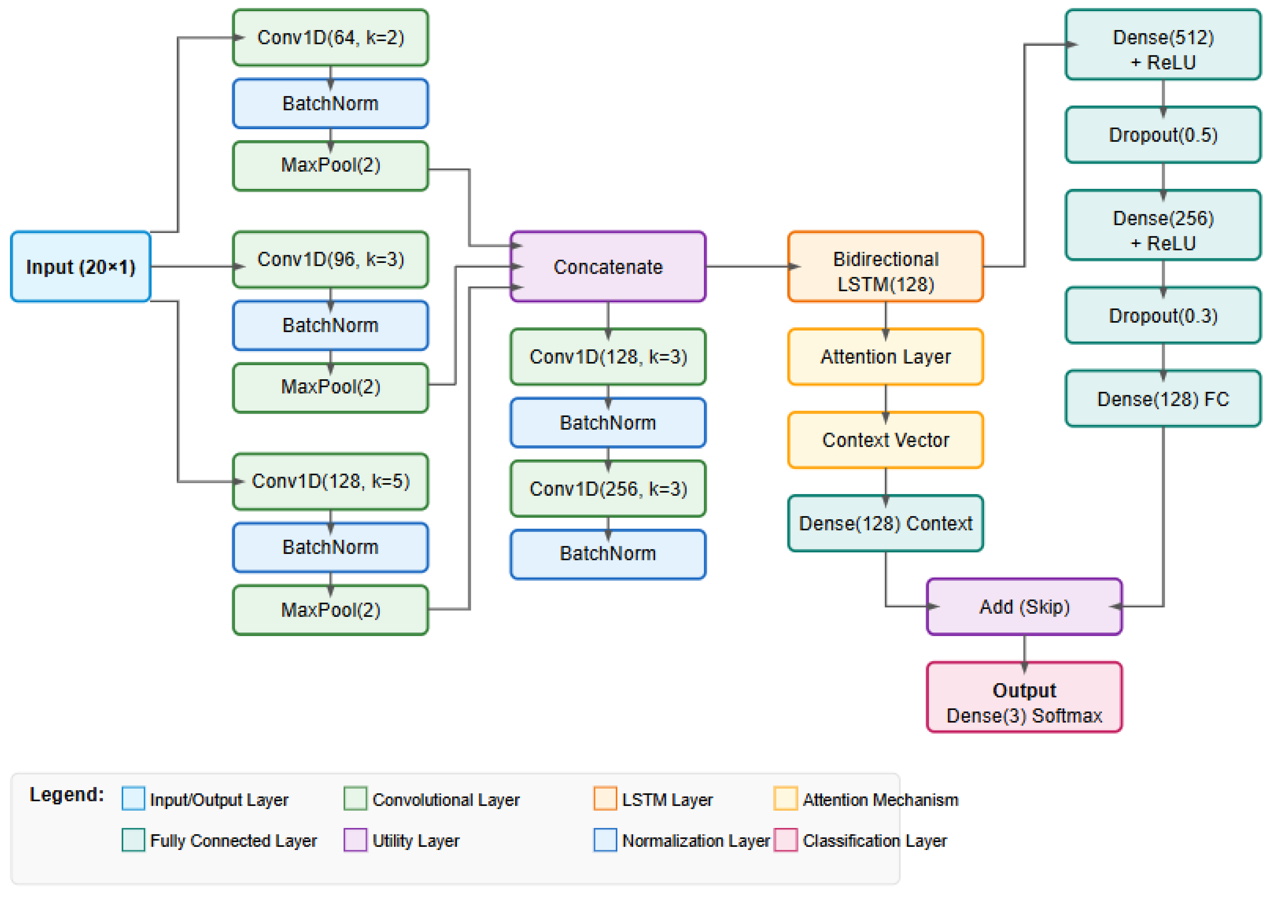
Class-specific analysis reveals that Version 3 struggled particularly with the DA class under noisy conditions, achieving only 76.9% F1-score. Version 4 improved DA classification by 12.6% on the F1 metric. The confusion matrices further illustrate this improvement: Version 3 frequently misclassified DA as SS (16.2% error rate), while Version 4 reduced this specific error pattern by nearly 60%, bringing it down to 6.6%. This targeted improvement demonstrates that Version 4’s architectural enhancements specifically addressed the weaknesses identified in Version 3 when dealing with noisy data. The clear performance gap between Version 3 and Version 4 on noisy datasets led us to adopt Version 4 as our proposed architecture. Several key enhancements contributed to its superior noise resilience: enhanced multi-scale feature extraction with varying filter counts (64, 96, and 128) across different kernel sizes (2, 3, and 5) allows better distinction between signal and noise at multiple resolutions; the attention mechanism dynamically focuses on informative signal parts while ignoring noisy regions; skip connections maintain gradient flow and preserve information across network depth; L2 regularization prevents overfitting to noise patterns; and the adaptive learning rate scheduler allows for better parameter fine-tuning during training. Testing on noisy datasets provided critical insights that shaped our final architecture: real-world data rarely comes in clean forms, and the superior performance on the COMBO dataset suggests Version 4 is more suitable for practical deployment; specific improvements in the DA class indicate that Version 4 addressed key weaknesses in discriminating between similar classes under noisy conditions; the remarkable improvement in temporal stability under noise suggests that Version 4 will produce more consistent predictions in variable real-world conditions; and balanced improvements across all noise types demonstrate that Version 4’s enhancements represent general improvements in noise resilience.

Based on comprehensive evaluations, Version 4 clearly emerges as our proposed architecture for the hybrid CNN–RNN model. Its exceptional performance on the COMBO dataset, which most closely resembles real-world conditions with mixed noise profiles, provides strong evidence for its practical utility in classifying CA, DA, and SS classes in noisy environments. The architectural enhancements implemented in Version 4 directly address the limitations identified in earlier versions, resulting in a model that is not only more accurate but also significantly more robust and reliable under challenging conditions.

5.4. Comparative Analysis with State-of-the-Art Approaches

To establish the superiority of our proposed solution, we conducted extensive comparative analysis between our hybrid CNN–LSTM architecture (Version 4) and several state-of-the-art approaches. This comprehensive evaluation focused on the challenging COMBO dataset, which represents real-world conditions with mixed noise profiles (60% BASE, 20% GAUSS, 20% RAND).

Our comparative analysis encompassed three key dimensions: (1) comparison of different classification algorithms using our proposed hybrid features, (2) comparison between our hybrid features and Riemannian geometry-based features across multiple classifiers, and (3) ablation study on the contribution of time-domain versus frequency-domain features.

The comparative analysis reveals several critical insights regarding the performance of our proposed solution:

1. Feature Domain Synergy: Our ablation study (

Table 15. Performance comparison of different approaches on COMBO dataset.

Approach	Accuracy	F1-Score (Macro)	Temporal Stability Coefficient
Feature-Domain Analysis with Proposed CNN–LSTM (V4)
Time-Domain Features Only	0.875	0.872	0.143
Frequency-Domain Features Only	0.882	0.879	0.135
Proposed Hybrid Features + Classification Methods
Hybrid Features + SVM	0.863	0.857	0.176
Hybrid Features + RF	0.879	0.875	0.148
Hybrid Features + ERT	0.883	0.879	0.142
Hybrid Features + GTB	0.891	0.887	0.138
Hybrid Features + AdaBoost	0.871	0.865	0.159
Hybrid Features + Ensemble	0.896	0.892	0.125
Riemannian Geometry Features + Classification Methods [19,20]
Riemannian Features + RF	0.842	0.836	0.183
Riemannian Features + ERT	0.851	0.845	0.175
Riemannian Features + GTB	0.865	0.859	0.164
Riemannian Features + AdaBoost	0.832	0.826	0.192
Riemannian Features + Ensemble	0.877	0.872	0.157
Proposed Approach
Hybrid Features + Proposed CNN–LSTM (Version 4)	0.927	0.924	0.089
Additional Deep Learning Architectures
Hybrid Features + Transformer (8-head, 256-dim)	0.898	0.894	0.132
Hybrid Features + Temporal CNN (dilated conv)	0.887	0.883	0.146
Hybrid Features + CNN–GRU	0.903	0.899	0.118

,

Table 16. Class-specific F1-scores for top-performing approaches.

Approach	CA	DA	SS	Macro Average
Time-Domain Features Only + CNN–LSTM (V4)	0.889	0.835	0.892	0.872
Frequency-Domain Features Only + CNN–LSTM (V4)	0.895	0.847	0.895	0.879
Hybrid Features + Ensemble	0.902	0.863	0.911	0.892
Riemannian Features + Ensemble	0.884	0.843	0.889	0.872
Riemannian Features + GTB	0.872	0.829	0.876	0.859
Hybrid Features + GTB	0.897	0.857	0.907	0.887
Hybrid Features + Transformer	0.908	0.869	0.905	0.894
Hybrid Features + Temporal CNN	0.895	0.852	0.902	0.883
Hybrid Features + CNN–GRU	0.915	0.873	0.909	0.899
Hybrid Features + Proposed CNN–LSTM (V4)	0.940	0.895	0.938	0.924

and

Table 17. Class-specific metrics for feature-domain analysis with CNN–LSTM (V4).

Feature Set	Metric	CA	DA	SS	Macro Average
Time-Domain Only	Precision	0.884	0.842	0.897	0.874
	Recall	0.895	0.828	0.887	0.870
	F1-Score	0.889	0.835	0.892	0.872
Frequency-Domain Only	Precision	0.891	0.853	0.899	0.881
	Recall	0.898	0.841	0.891	0.877
	F1-Score	0.895	0.847	0.895	0.879
Hybrid Features (Proposed)	Precision	0.938	0.898	0.943	0.926
	Recall	0.943	0.893	0.934	0.923
	F1-Score	0.940	0.895	0.938	0.924

) clearly demonstrates the synergistic benefit of combining time- and frequency-domain features. Using time-domain features alone achieves 87.5% accuracy and 0.872 F1-score, while frequency-domain features alone achieve 88.2% accuracy and 0.879 F1-score. However, our hybrid approach that combines both domains reaches 92.7% accuracy and 0.924 F1-score, representing significant improvements of 5.2 and 4.5 percentage points, respectively, over time-domain features alone;

2. Class-Specific Feature Contributions: Table 17 reveals interesting patterns in how different feature domains contribute to class discrimination. For the DA class, which is consistently the most challenging to classify, frequency-domain features (F1: 0.847) outperform time-domain features (F1: 0.835) by 1.2 percentage points. However, the hybrid approach (F1: 0.895) surpasses frequency-only features by an additional 4.8 percentage points, highlighting the complementary nature of these feature sets;

3. Temporal Stability Enhancement: The hybrid feature approach dramatically improves temporal stability (coefficient: 0.089) compared to using either time-domain (0.143) or frequency-domain features (0.135) alone. This 37.8% improvement in stability over frequency-only features demonstrates how the combined feature set provides more consistent classification across temporal variations in the signal;

4. Superior Overall Performance: Our proposed approach (Hybrid Features + CNN–LSTM Version 4) consistently outperforms all alternative methods across all evaluation metrics. It achieves 92.7% accuracy and 0.924 F1-score on the COMBO dataset, representing improvements of 3.1 percentage points in accuracy and 3.2 percentage points in F1-score over the next best alternative (Hybrid Features + Ensemble);

5. Hybrid Feature Advantage: The results clearly demonstrate that our hybrid time- and frequency-domain feature-extraction strategy consistently outperforms Riemannian geometry-based features across all classification methods. For instance, when using the same ensemble classification approach, our hybrid features achieve a 1.9 percentage point higher accuracy and 2.0 percentage point higher F1-score compared to Riemannian features;

6. Architecture Advantage: When comparing approaches using the same feature set, our proposed CNN–LSTM architecture significantly outperforms traditional machine learning approaches. This indicates that the advanced architectural elements in our model—multi-scale feature extraction, attention mechanism, skip connections, and regularization techniques—are particularly effective at leveraging the information contained in our hybrid features;

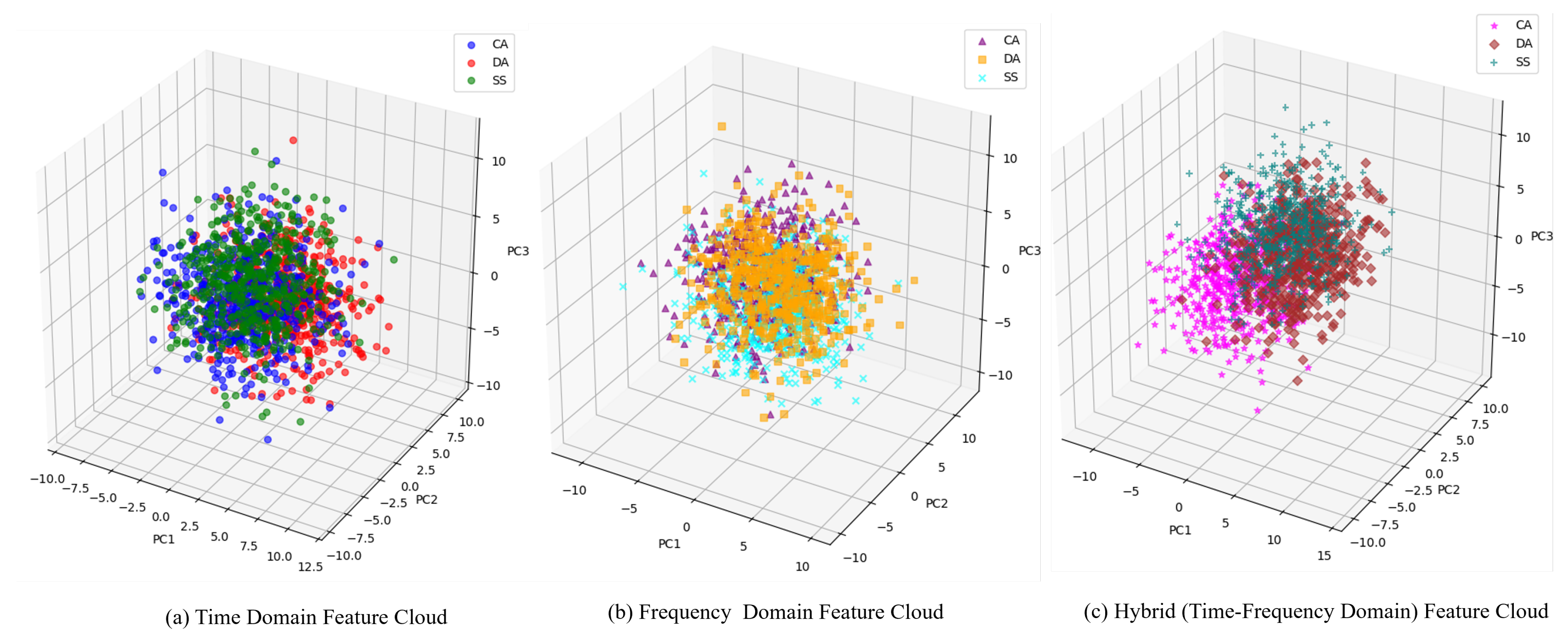
7. Feature Complementarity: The substantial performance improvement from combining time- and frequency-domain features suggests that these feature sets capture complementary aspects of the signal. Time-domain features (including statistical measures like mean, standard deviation, variance, skewness, kurtosis, maximum, minimum, peak-to-peak amplitude, root mean square, zero crossings, and Hjorth parameters) capture temporal patterns and amplitude characteristics, while frequency-domain features (power metrics across different frequency bands, relative powers, spectral edge frequency, mean frequency, and spectral entropy) capture spectral characteristics;

8. Noise Resilience: The consistent superiority across all metrics on the challenging COMBO dataset, which contains mixed noise profiles, confirms the exceptional noise resilience of our proposed approach—a critical factor for real-world deployability. The hybrid feature set appears particularly robust to noise, likely because certain features remain discriminative even when others are corrupted by noise;

9. Additional Deep Learning Architecture Comparisons: To provide a comprehensive evaluation against modern deep learning approaches, we compared our proposed method with several advanced architectures. The Transformer architecture with 8-head multi-head attention and 256 embedding dimensions achieved 89.8% accuracy and 0.894 F1-score, demonstrating strong performance but falling short of our hybrid CNN–LSTM approach by 2.9 percentage points in accuracy. The Temporal CNN with dilated convolutions, designed specifically for temporal pattern recognition, achieved 88.7% accuracy and 0.883 F1-score. Interestingly, the CNN–GRU hybrid architecture performed competitively with 90.3% accuracy and 0.899 F1-score, representing the closest competitor among the deep learning baselines. However, our proposed CNN–LSTM architecture still outperformed it by 2.4 percentage points in accuracy and 2.5 percentage points in F1-score. The superior performance of our approach can be attributed to the specific combination of bidirectional LSTM with attention mechanism, which better captures the temporal dependencies in EEG signals compared to the unidirectional nature of GRU units, and the multi-scale CNN feature extraction that is optimized for our hybrid feature representation.

The comprehensive evaluation firmly establishes our proposed architecture with hybrid features as the superior choice for classifying CA, DA, and SS classes, offering unprecedented accuracy, stability, and noise resilience for reliable deployment in real-world scenarios. The synergistic combination of complementary time- and frequency-domain features with our specialized CNN–LSTM architecture creates a powerful solution that substantially outperforms all alternative approaches.

5.5. Discussion

To validate the practical applicability of our proposed real-time pilot attention state prediction system, external validation using EEG data collected during actual flight training or cockpit sitting conditions—rather than solely relying on LOFT-based simulations—is essential. While our hybrid CNN–LSTM architecture demonstrates robust performance on simulation data with superior accuracy across diverse noise conditions, the transition to operational environments presents unique challenges, including electromagnetic interference, cockpit vibrations, and varying environmental conditions that may affect EEG signal quality. Future research must focus on developing miniaturized, flight-certified EEG acquisition systems capable of reliable operation in actual cockpit environments, establishing collaborative protocols with aviation training institutions for controlled data collection during real flight scenarios, and investigating transfer learning approaches that could adapt our model to authentic flight conditions with minimal additional training data. This validation pathway, while requiring multi-year planning and regulatory approval processes, represents the critical foundation necessary before implementing any intervention mechanisms in operational aviation settings.

Building upon successful real-world validation, the real-time detection of attention states (CA, DA, SS) enables several intervention mechanisms that could fundamentally transform aviation safety protocols. When channelized attention is detected, adaptive alerting systems could generate targeted notifications to redirect pilot focus toward neglected instruments or critical flight parameters, while diverted attention episodes could trigger workload redistribution protocols that temporarily assume control of non-critical automated systems, allowing pilots to focus on essential operations. Perhaps most critically, startle/surprise state detection could initiate immediate cognitive reset protocols, including standardized callouts, simplified decision trees, or emergency checklists designed to help pilots recover from cognitive paralysis during critical moments. These interventions extend beyond individual pilot support to enhance crew resource management through predictive communications to co-pilots or air traffic control, creating distributed awareness networks that compensate for cognitive limitations before critical situations develop. Implementation requires careful human factors engineering following established aviation human–machine interface design principles, ensuring that technological augmentation enhances rather than interferes with pilot performance while maintaining appropriate transparency and pilot authority over system responses. Therefore, our future work will focus on three interconnected research streams: (1) conducting multi-site validation studies in actual flight training environments to establish ecological validity and system robustness, (2) developing and testing intervention protocols through controlled human factors experiments to optimize alert timing, modality, and intensity, and (3) creating comprehensive pilot acceptance and workload assessment frameworks to ensure that intervention mechanisms enhance rather than compromise flight safety and operational efficiency.

6. Conclusions

Our research presents a novel hybrid CNN–LSTM architecture for robust classification of CA, DA, and SS classes in challenging, noisy environments. The proposed approach systematically addresses key challenges in pilot attention monitoring through thoughtful design and comprehensive validation using the publicly available “Reducing Commercial Aviation Fatalities” dataset. The experimental results demonstrate that our approach achieves superior performance across all evaluation metrics compared to existing state-of-the-art methods, with notable improvements in temporal stability and noise resilience under controlled experimental conditions.

The success of our approach stems from two key innovations validated through our experimental framework. First, our hybrid feature-extraction strategy combines complementary information from both time and frequency domains, providing a comprehensive representation of EEG signals that captured the neural signatures of critical pilot attention states within our dataset. Our ablation studies clearly demonstrated the synergistic benefit of this combination, with hybrid features achieving 92.7% accuracy compared to 87.5% for time-domain features alone and 88.2% for frequency-domain features alone. Second, our specialized CNN–LSTM architecture effectively leverages these hybrid features through multi-scale convolution, attention mechanisms, and skip connections, enabling robust pattern recognition even under the artificially generated noise conditions tested in our study.

Our experimental validation focused on establishing proof-of-concept performance under controlled conditions using synthetic noise profiles (Gaussian, random, and combined noise). The model demonstrated consistent performance across these noise variants, with the COMBO dataset (representing mixed noise conditions) showing 92.7% accuracy and significant improvements in temporal stability coefficient (0.089) compared to baseline approaches. The architecture progression from Version 1 to Version 4 showed systematic improvements, with the final model achieving superior performance across all three attention states: CA (94.0% F1-score), DA (89.5% F1-score), and SS (93.8% F1-score). While these results are promising, several important limitations must be acknowledged. Our evaluation was conducted on a single dataset with 18 participants, and we did not perform cross-subject validation to assess generalizability across different pilot populations. The noise resilience testing, while comprehensive within our experimental design, was limited to synthetic noise profiles and may not fully represent the complex artifacts encountered in operational aviation environments. Additionally, our computational efficiency analysis was limited to training metrics (epochs and parameters), without a detailed assessment of inference speed or memory requirements that would be critical for real-time aviation applications. The interpretability of our model decisions, while enhanced by our hybrid feature approach using neurophysiologically meaningful features, was not extensively analyzed to determine which specific features drive classification decisions for each attention state. This represents an important area for future investigation, particularly given the safety-critical nature of aviation applications, where understanding model reasoning is essential for regulatory approval and operational trust.

Future research directions should prioritize several key areas to advance this work toward practical implementation. Cross-subject validation studies are essential to establish generalizability across different pilot populations and training backgrounds. Computational efficiency optimization and real-time inference analysis on aviation-grade hardware would provide crucial insights for operational deployment feasibility. Feature importance analysis and explainable AI techniques could enhance model interpretability by identifying which neurophysiological markers are most critical for each attention state classification. Additionally, validation using real flight data with naturally occurring artifacts, rather than synthetic noise, would provide a more realistic assessment of model robustness. Investigating transfer learning approaches could enable model adaptation to new pilots with minimal calibration, while incorporating self-supervised pre-training might enhance performance in scenarios with limited labeled data. The work presented here establishes a strong foundation for EEG-based pilot attention monitoring, demonstrating the potential of hybrid feature extraction and CNN–LSTM architectures within controlled experimental conditions. However, the translation from laboratory validation to operational aviation systems will require addressing the limitations identified and conducting more extensive real-world testing to ensure the reliability and safety required for this critical application domain.

References

1. Jones, D.G.; Endsley, M.R. Sources of situation awareness errors in aviation. Aviat. Space Environ. Med. 1996, 67, 507–512. [Google Scholar] [PubMed]
2. International Air Transport Association. 2021 Safety Report Edition; International Air Transport Association: Montreal, QC, Canada, 2022. [Google Scholar]
3. International Air Transport Association. Loss of Control In-Flight Accident Analysis Report 2019 Edition; International Air Transport Association: Montreal, QC, Canada, 2019. [Google Scholar]
4. Commercial Aviation Safety Team. SE211: Airplane State Awareness—Training for Attention Management. Available online: http://www.skybrary.aero/index.php/SE211:_Airplane_State_Awareness_-_Training_for_Attention_Management_(R-D) (accessed on 3 March 2025).
5. Yen, J.; Hsu, C.; Yang, H.; Ho, H. An Investigation of Fatigue Issues on Different Flight Operations. J. Air Transp. Manag. 2009, 15, 236–240. [Google Scholar] [CrossRef]
6. Hankins, T.; Wilson, G. A Comparison of Heart Rate, Eye Activity, EEG and Subjective Measures of Pilot Mental Workload during Flight. Aviat. Space Environ. Med. 1998, 69, 360–367. [Google Scholar] [PubMed]
7. Boksem, M.; Tops, M. Mental Fatigue: Costs and Benefits. Brain Res. Rev. 2008, 59, 125–139. [Google Scholar] [CrossRef]
8. Bigdely-Shamlo, N.; Mullen, T.; Kothe, C.; Su, K.; Robbins, K. The PREP Pipeline: Standardized Preprocessing for Large-Scale EEG Analysis. Front. Neuroinform. 2015, 9, 16. [Google Scholar] [CrossRef]
9. Fló, A.; Gennari, G.; Benjamin, L.; Dehaene-Lambertz, G. Automated Pipeline for Infants Continuous EEG (APICE): A Flexible Pipeline for Developmental Cognitive Studies. Dev. Cogn. Neurosci. 2022, 54, 101077. [Google Scholar] [CrossRef]
10. Kaggle. Reducing Commercial Aviation Fatalities. Available online: https://www.kaggle.com/competitions/reducing-commercial-aviation-fatalities/overview (accessed on 3 March 2025).
11. Roza, V.; Postolache, O. Multimodal Approach for Emotion Recognition Based on Simulated Flight Experiments. Sensors 2019, 19, 5516. [Google Scholar] [CrossRef]
12. Han, S.; Kwak, N.; Oh, T.; Lee, S. Classification of Pilots’ Mental States Using a Multimodal Deep Learning Network. Biocybern. Biomed. Eng. 2020, 40, 324–336. [Google Scholar] [CrossRef]
13. Alreshidi, I.; Moulitsas, I.; Jenkins, K. Miscellaneous EEG Preprocessing and Machine Learning for Pilots’ Mental States Classification: Implications; Association for Computing Machinery: New York, NY, USA, 2022. [Google Scholar]
14. Jas, M.; Engemann, D.; Bekhti, Y.; Raimondo, F.; Gramfort, A. Autoreject: Automated Artifact Rejection for MEG and EEG Data. Neuroimage 2017, 159, 417–429. [Google Scholar] [CrossRef]
15. Bonassi, A.; Ghilardi, T.; Gabrieli, G.; Truzzi, A.; Doi, H.; Borelli, J.; Lepri, B.; Shinohara, K.; Esposito, G. The Recognition of Cross-Cultural Emotional Faces Is Affected by Intensity and Ethnicity in a Japanese Sample. Behav. Sci. 2021, 11, 59. [Google Scholar] [CrossRef]
16. Pousson, J.; Voicikas, A.; Bernhofs, V.; Pipinis, E.; Burmistrova, L.; Lin, Y.; Griškova-Bulanova, I. Spectral Characteristics of EEG during Active Emotional Musical Performance. Sensors 2021, 21, 7466. [Google Scholar] [CrossRef] [PubMed]
17. Harrivel, A.; Stephens, C.; Milletich, R.; Heinich, C.; Last, M.; Napoli, N.; Abraham, N.; Prinzel, L.; Motter, M.; Pope, A. Prediction of Cognitive States during Flight Simulation Using Multimodal Psychophysiological Sensing. In Proceedings of the AIAA Information Systems—AIAA Infotech at Aerospace, Grapevine, TX, USA, 9–13 January 2017. [Google Scholar]
18. Hasan, M.J.; Shon, D.; Im, K.; Choi, H.K.; Yoo, D.S.; Kim, J.M. Sleep State Classification Using Power Spectral Density and Residual Neural Network with Multichannel EEG Signals. Appl. Sci. 2020, 10, 7639. [Google Scholar] [CrossRef]
19. Wu, E.; Peng, X.; Zhang, C.; Lin, J.; Sheng, R. Pilots’ Fatigue Status Recognition Using Deep Contractive Autoencoder Network. IEEE Trans. Instrum. Meas. 2019, 68, 3907–3919. [Google Scholar] [CrossRef]
20. Binias, B.; Myszor, D.; Cyran, K. A Machine Learning Approach to the Detection of Pilot’s Reaction to Unexpected Events Based on EEG Signals. Comput. Intell. Neurosci. 2018, 2018, 2703513. [Google Scholar] [CrossRef]
21. Ji, L.; Yi, L.; Li, H.; Han, W.; Zhang, N. Detection of Pilots’ Psychological Workload during Turning Phases Using EEG Characteristics. Sensors 2024, 24, 5176. [Google Scholar] [CrossRef]
22. Feng, C.; Liu, S.; Wanyan, X.; Dang, Y.; Wang, Z.; Qian, C. β-wave-based exploration of sensitive EEG features and classification of situation awareness. Aeronaut. J. 2024, 128, 2561–2576. [Google Scholar] [CrossRef]
23. Barachant, A.; Bonnet, S.; Congedo, M.; Jutten, C. Multiclass Brain-Computer Interface Classification by Riemannian Geometry. IEEE Trans. Biomed. Eng. 2012, 59, 920–928. [Google Scholar] [CrossRef]
24. Majidov, I.; Whangbo, T. Efficient Classification of Motor Imagery Electroencephalography Signals Using Deep Learning Methods. Sensors 2019, 19, 1736. [Google Scholar] [CrossRef]
25. Johnson, M.; Blanco, J.; Gentili, R.; Jaquess, K.; Oh, H.; Hatfield, B. Probe-Independent EEG Assessment of Mental Workload in Pilots. In Proceedings of the International IEEE/EMBS Conference on Neural Engineering, NER, Montpellier, France, 22–24 April 2015; Volume 2015, pp. 581–584. [Google Scholar]
26. Harrivel, A.; Liles, C.; Stephens, C.; Ellis, K.; Prinzel, L.; Pope, A. Psychophysiological Sensing and State Classification for Attention Management in Commercial Aviation. In Proceedings of the AIAA Infotech @ Aerospace Conference, Crew Systems and Aviation Operations Branch, NASA Langley Research Center, Hampton, VA, USA, 4–8 January 2016. [Google Scholar]
27. Cheng, L.; Shen, Y.C.; He, Q.; Zhang, M.J. Spying with a pilot’s eye: Using eye tracking to investigate pilots’ attention allocation and workload during helicopter autorotative gliding. Heliyon 2024, 10, e35872. [Google Scholar] [CrossRef]
28. Samy, S.; Gedam, V.V.; Karthick, S. The drowsy driver detection for accident mitigation using facial recognition system. Life Cycle Reliab. Saf. Eng. 2025, 14, 299–311. [Google Scholar] [CrossRef]
29. Alreshidi, I.; Moulitsas, I.; Jenkins, K.W. Multimodal Approach for Pilot Mental State Detection Based on EEG. Sensors 2023, 23, 7350. [Google Scholar] [CrossRef] [PubMed]
Figure 1. Proposed methodology.
Information 16 00503 g001
Figure 2. Proposed CNN–LSTM architecture.
Information 16 00503 g002
Figure 3. Detailed statistics on the dataset.
Information 16 00503 g003
Figure 4. PCA-applied feature space for visualization purposes for (a) time-domain features, (b) frequency-domain features, and (c) hybrid features, which consist of time- and frequency-domain features.
Information 16 00503 g004