Global Navigation Satellite System Spoofing Attack Detection Using Receiver Independent Exchange Format Data and Long Short-Term Memory Algorithm

Abstract

Global Navigation Satellite Systems (GNSS) are widely used for positioning, navigation, and timing (PNT) applications, making them a critical infrastructure component. However, GNSS signals and receivers are vulnerable to several attacks that can expose the users to serious threats. The GNSS spoofing attack, for example, is one of the most widespread in this domain and is used to manipulate positioning and timing data by transmitting counterfeit signals. Thus, in this study, we propose a method for analyzing and detecting anomalies in RINEX observation data that is associated with spoofing attacks. The proposed method is based on Long Short-Term Memory (LSTM) networks and focuses on the observation parameters defined by the RINEX standard, which are computed in the Measurements block and subsequently used in the Navigation block of a GNSS receiver architecture. Attack detection involves processing GNSS observation codes and learning the temporal dependencies necessary to identify anomalies associated with GNSS signal spoofing. During the testing phase, the proposed method was applied to GNSS observation codes affected by spoofing, using an LSTM-based reconstruction approach. An ensemble strategy across grouped observation codes was used to identify temporal inconsistencies indicative of anomalies.

1. Introduction

Global Navigation Satellite Systems (GNSS) are satellite-based navigation systems that provide geospatial positioning and synchronization data to users worldwide [1,2]. These systems enable accurate determination of location, velocity, and time synchronization, making them essential for a wide range of applications such as civilian navigation, financial services, autonomous vehicles, network protocols, military applications, critical infrastructure, and so on [3].

Depending on the service coverage area offered by navigation systems, we identify the following types [4]:

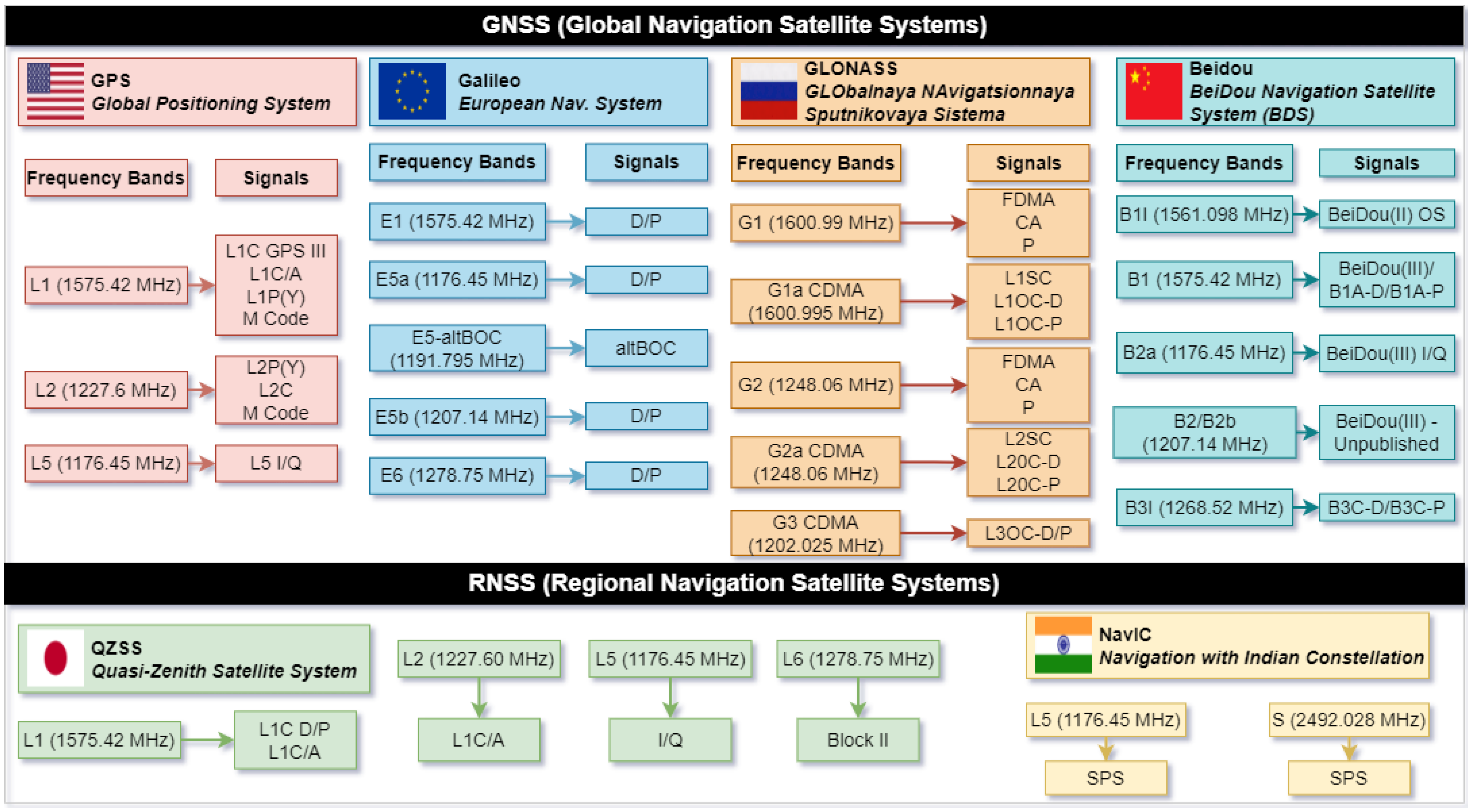
• Global Navigation Satellite Systems (GNSS);
• Regional Navigation Satellite Systems (RNSS);
• Satellite-Based Augmentation Systems (SBAS).

Global Navigation Satellite Systems consists of four constellations of navigation satellites providing global coverage as follows:

• GPS: The Global Positioning System (the current name of the Navstar system) is the system owned by the United States of America that became operational in 1995. The system comprises satellites located in the Medium Earth Orbit (MEO) and provides very accurate navigation and synchronization data [5,6].
• Beidou: The Chinese Global Navigation Satellite System is owned and developed by China, which includes geostationary (GEO), MEO, and Inclined Geosynchronous Orbit (IGSO) satellites [7,8]. The system is designed to provide very accurate navigation and synchronization data.
• Galileo: This is the fully operational European navigation system that emerged at the initiative of the European Space Agency (ESA). The system has a recent history and is in continuous development. It became fully operational in 2016 and is composed of satellites placed in MEO [9].
• GLONASS: The GLObalnaya NAvigatsionnaya Sputnikovaya Sistema is the system owned by the Russian Federation that became fully operational in 1995 and is composed of satellites in MEO [10].

Regional Navigation Satellite Systems consists of two constellations of navigation satellites providing regional coverage as follows:

• NavIC/IRNSS: Navigation with Indian Constellation is the system owned by India and is composed of eight satellites with IGSO and GEO orbits [11].
• QZSS: Quasi-Zenith Satellite System Chinese is the system owned by Japan and is composed also from satellites with IGSO and GEO orbits [12,13].

Satellite-Based Augmentation Systems are complementary navigation satellite systems that have been developed to improve the accuracy of global and regional navigation systems [14]. These systems consist of geostationary satellites that use the same signal structure and frequency bands as global and regional systems.

Based on data provided by official authorities regarding the technical specifications of each system [15,16,17,18], Figure 1 shows an overview of GNSS, RNSS, and SBSS as well as the number of satellites (operational at this moment), the system orbit, the satellites’ altitudes, and the orbit period (for satellites placed on MEO and IGSO).

Each navigation system consists of three main segments [2,19]:

• Space segment: Consists of the navigation satellites that orbit the Earth and transmit signals to users.
• Control segment: Includes monitoring and control ground stations that ensure the integrity and accuracy of the satellites.
• User segment: Includes all devices that have a built-in navigation sensor, such as smartphones, airplanes, and so on, which process the signals to determine location.

From the space segment perspective, each navigation system transmits data in different frequency bands. There are cases where some systems share the same frequency band. For example, the frequency band commonly referred to as L1 (1575.42 MHz) for civilian applications is one of the most widely used and is found in GPS, Galileo, Beidou, and QZSS. These frequency bands are used to transmit navigation data using navigation signals, which can be either unencrypted or encrypted [20]. Most encrypted signals have a specific destination, usually for military use or special applications. Thus, unencrypted signals for civilian use may be vulnerable and expose users to threats. Based on information provided by technical specifications of each constellation [15,16,17,18], an overview of the main frequency bands and signals used in GNSS and RNSS is given in Figure 2.

From the user segment perspective, navigation receivers are inherently vulnerable to some major cybersecurity attacks due to several factors:

• Most civilian navigation signals are broadcast in an unencrypted format, making them vulnerable to signal manipulation. This claim is supported by several recent studies [20,21,22] in which the authors experimented with various techniques and methods for manipulating unencrypted civilian signals. Unlike military signals, which use encryption and authentication mechanisms, civilian receivers cannot distinguish between legitimate and spoofed navigation signals.
• Navigation signals come from high altitudes and reach receivers at very low power levels (typically around −130 dBm) [20]. This makes them susceptible to interference and jamming by false signals, which can be transmitted at higher power from terrestrial sources.
• Many GNSS receivers still operate on single-frequency signals (e.g., GPS L1 only), which makes them more vulnerable to spoofing [23]. Multi-frequency receivers using L1, L2, and L5 signals can improve resilience by cross-checking signals from different bands, but such protection is not yet widespread.

Nowadays, a spoofing attack on navigation sensors can be easily performed by using a navigation signal sample and transmission equipment. The evolution of low-cost solutions such as Software Defined Radio (SDR) technologies and the availability of open-source tools for generating and manipulating these signals have significantly reduced the technical barriers for attackers [24]. As a consequence, some recent events show how dangerous these attacks are and the damage they can cause. In 2017, there was a series of drone strikes in Syria in which Russian military forces were accused of using GNSS spoofing attacks. In the following year, a merchant vessel in the Black Sea fell victim to a spoofing attack, resulting in signal loss and incorrect positioning [25]. As a consequence, the ship drifted off course, nearly colliding with another vessel. OpsGroup data indicates that GNSS spoofing is most prevalent in the eastern Mediterranean, affecting regions such as Israel, Lebanon, Cyprus, and Egypt. Elevated spoofing activity is also reported near the Black Sea, in western Russia, and along the India–Pakistan border [26]. The situation has escalated further in 2024, particularly in the aviation sector. Recent findings by SkAI Data Services, in partnership with the University of Applied Sciences in Zurich, indicate a significant surge in GNSS spoofing incidents affecting civil aviation [27]. The number of affected flights increased from a few dozen per day in February to over 1100 daily by August 2024 [27]. Furthermore, The Wall Street Journal reported a notable incident in August 2024 involving a flight from New Delhi to New York, which experienced GPS spoofing that disrupted its navigation systems throughout the flight [28].

Furthermore, based on recent research, the multitude of complex spoofing techniques, as presented in [20], and some of them tested in [21,22,29], further reinforces the necessity for developing diversified and multi-layered (based on the Diversity and Layering principle from cybersecurity) countermeasures tailored to different levels of a GNSS sensor architecture. In [22], for example, the authors tested a slow-drift spoofing attack designed to gradually deviate the positioning of autonomous vehicles without triggering detection mechanisms, using a method that closely mimics real satellite signals. Also, in a more complex scenario presented in [21], the authors used a distributed GNSS spoofing architecture in which multiple antennas simultaneously emit individual spoofing signals, overcoming the traditional angle-of-arrival-based anti-spoofing technique and demonstrating the potential for coordinated multi-node attacks. In [29], a gradual spoofing technique which progressively alters positioning data over time while remaining undetected by advanced anti-spoofing filters such as RAIM or parameter consistency checks was tested. All of these studies illustrate the increasing level of sophistication that can be achieved in the design and execution of GNSS spoofing attacks.

Spoofing attack detection can be achieved through anomaly detection applied to various signal parameters. This process involves identifying patterns that deviate from expected behaviors, which may indicate the presence of manipulation or deception. In this study, we propose an approach focused on the analysis of GNSS observation codes using a real-world dataset with high temporal resolution. To enable this, we developed a fully operational data acquisition and storage pipeline, capable of collecting GNSS observation codes from real signals, including those affected by spoofing events. The resulting dataset is structured according to the RINEX standard and comprises time series data characterized by temporal dependencies and data scarcity. To address these data characteristics, we employ a Long Short-Term Memory (LSTM)-based network designed to detect anomalies in the observation codes that may be generated by spoofing attacks.

The main contributions of this study are as follows:

• The development of a real-world data acquisition and storage pipeline for collecting high-resolution GNSS observation data, including both normal and spoofed signal traces, organized according to the RINEX standard.
• The integration of LSTM learning strategies over multiple observation codes per satellite signal, enhancing anomaly detection performance and improving resilience to spoofing variations.
• Validation of the method using real spoofed signals, achieving precision between 87.00% and 97.50% and recall between 75.35% and 79.2%, depending on the satellite and observation code, thereby demonstrating the method’s practical efficacy.

Therefore, the progress of the study for the rest of the paper is structured as follows: in Section 2, a description of the RINEX standard, the data format, and the observation parameters required for training and testing the LSTM algorithm is provided; in Section 3, a literature overview is provided; in Section 4, the architecture of the LSTM algorithm, the experimental setup, and the systems under test, along with their configurations for the training and testing process, are established; in Section 5, the results of model training and testing regarding its ability to detect anomalies associated with the spoofing attack are presented; and in Section 6, some conclusions and a comparison with similar methods and related research is conducted.

2. RINEX Standard

The Receiver Independent Exchange Format (RINEX) is an open standard designed for storing and exchanging raw GNSS observational data [30]. Developed by the Astronomical Institute of the University of Bern, RINEX ensures compatibility between different GNSS receivers and processing software, enabling efficient post-processing of navigation data from satellites.

RINEX has undergone multiple revisions to keep pace with advancements in GNSS technology, multi-constellation support, and additional data types [31]. The main versions of the standard are as follows:

• RINEX 2.x (1993–present): Originally developed to store GPS observations, this version was later extended to support GLONASS and Galileo. It introduced a simplified text-based structure, making it widely used for post-processing applications. Despite newer versions, RINEX 2.11 remains widely used, especially in legacy applications and receivers that do not support newer GNSS constellations.
• RINEX 3.x (2009–present): This version significantly improved multi-GNSS compatibility, allowing integration of GPS, GLONASS, Galileo, BeiDou, QZSS, SBAS, and IRNSS/NavIC data. It introduced additional observation types, including modernized GNSS signals such as GPS L5 and Galileo E5a/E5b. The latest revision, RINEX 3.05, addressed updates for new BeiDou and Galileo signals.
• RINEX 4.0 (2021–present): The latest version, RINEX 4.0, provides improved handling of high-rate data, extended support for new GNSS signals, and better integration with real-time processing workflows. This version was developed to improve efficiency in high accuracy applications such as Precise Point Positioning (PPP) and Real-Time Kinematic (RTK) positioning.

RINEX data are structured into several file types, each containing specific types of GNSS information [30]:

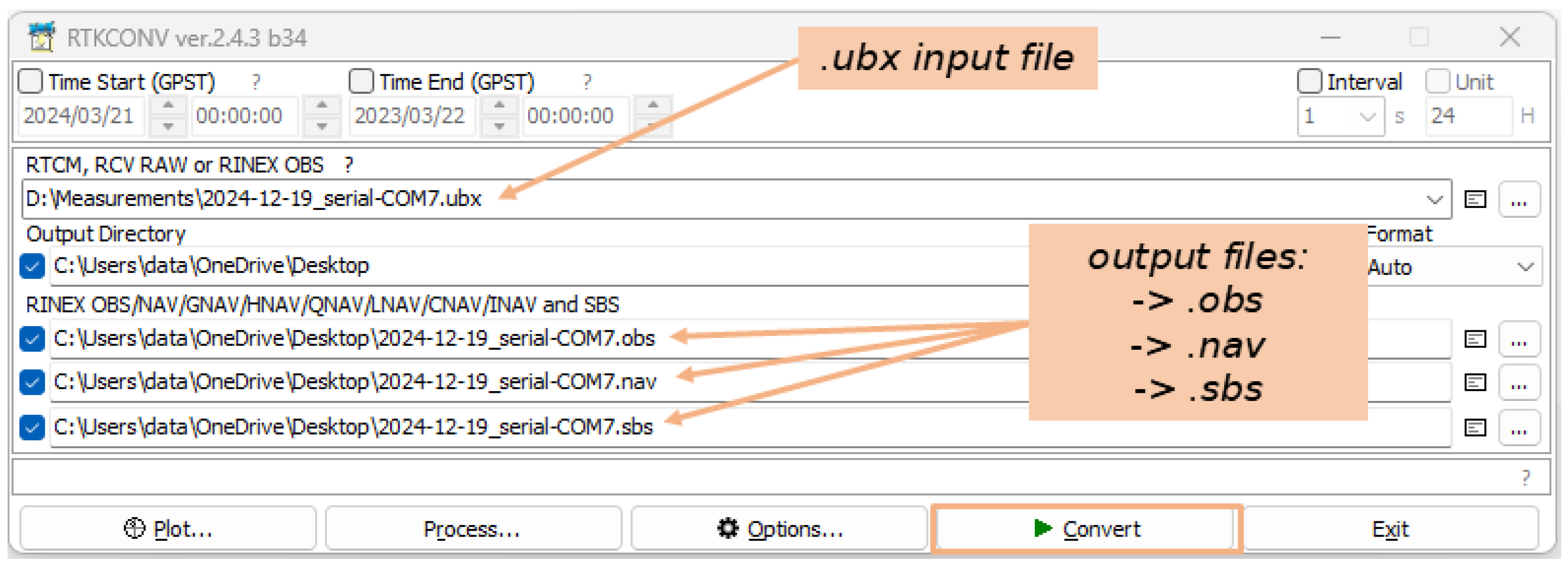
• Observation files (.obs extension): Contain raw GNSS observations, including Pseudorange, Carrier Phase, Doppler Shift, and Signal Strength.
• Navigation files (.nav extension): Store satellite ephemerides data necessary for computing positions.
• Meteorological files (.met extension): Include atmospheric data such as temperature, pressure, and humidity, which affect GNSS signal propagation.

Within the proposed mechanism, data from the observation files will be used. Due to the fact that the data in RINEX are standardized, the mechanism will be compatible with most versions. Thus, in the observational files, each navigation system is identified by the following notation: SNN; where S = satellite system identifier (G = GPS; R = GLONASS; E = Galileo; C = Beidou; S = SBAS; J = QZSS; and I = IRNSS), NN = satellite identification number (Pseudo-Random Noise Code–PRN number, used for GPS, Galileo, Beidou and IRNSS; Slot Number for GLONASS; PRN–100 for SBAS and QZSS; PRN–192 for QZSS).

Within the observation files, each identified satellite signal will be monitored using observation codes. The standard provides the following observation codes:

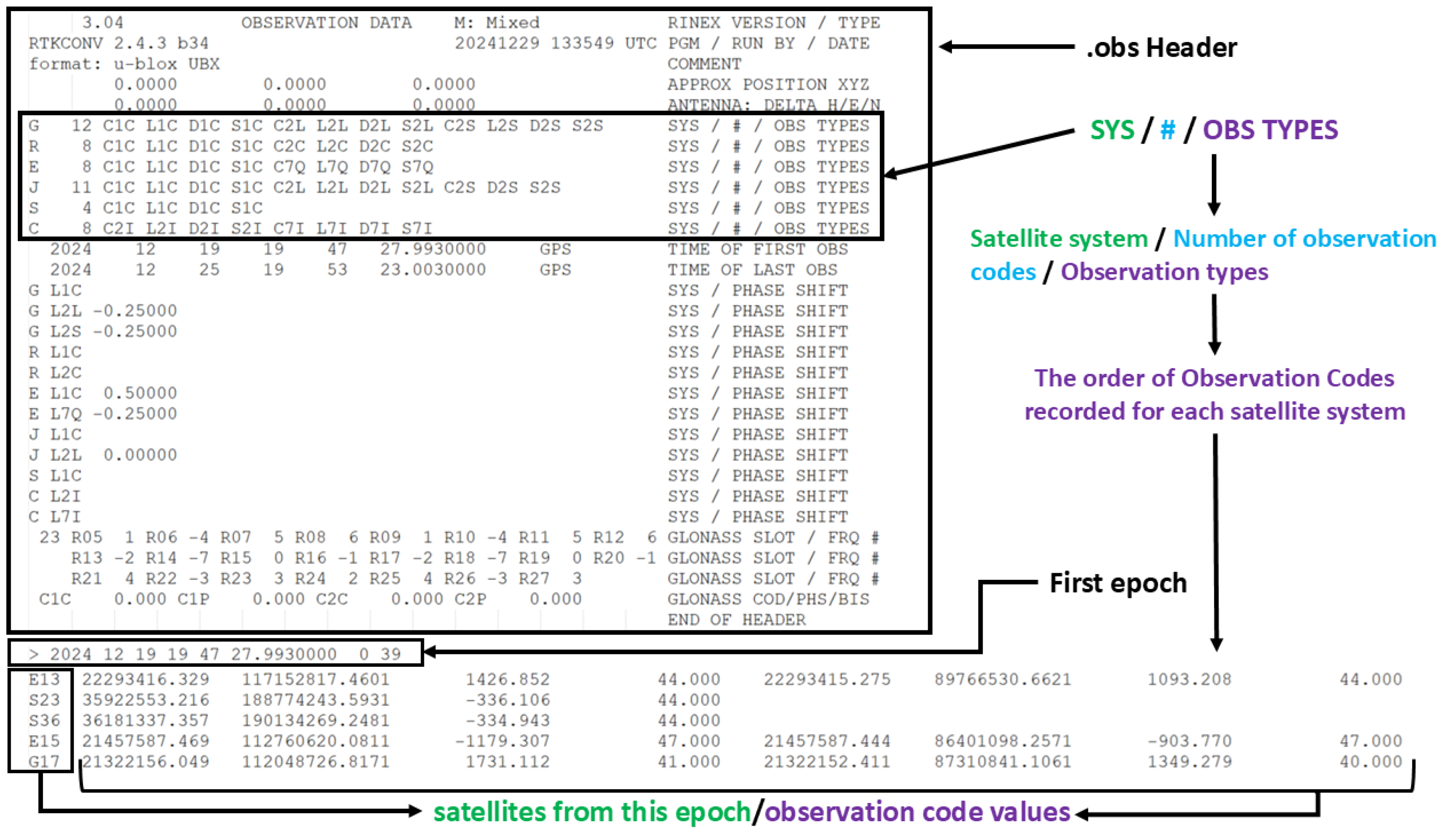
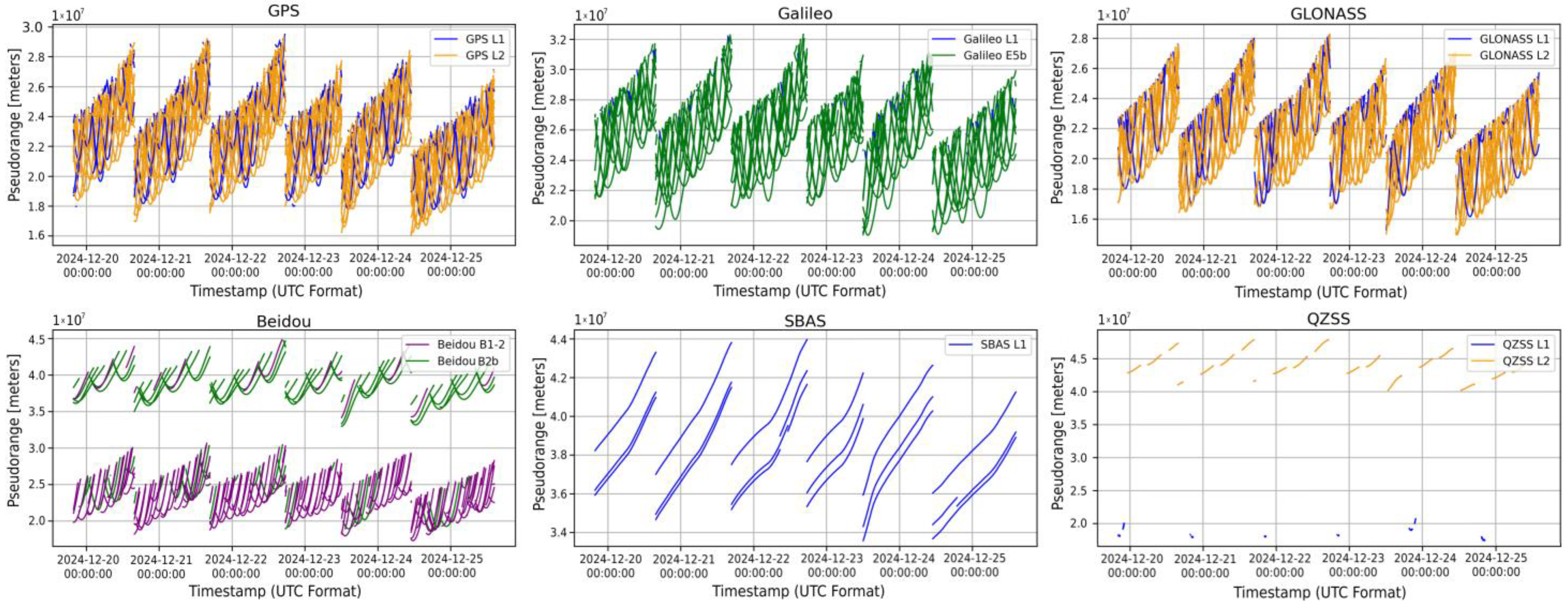
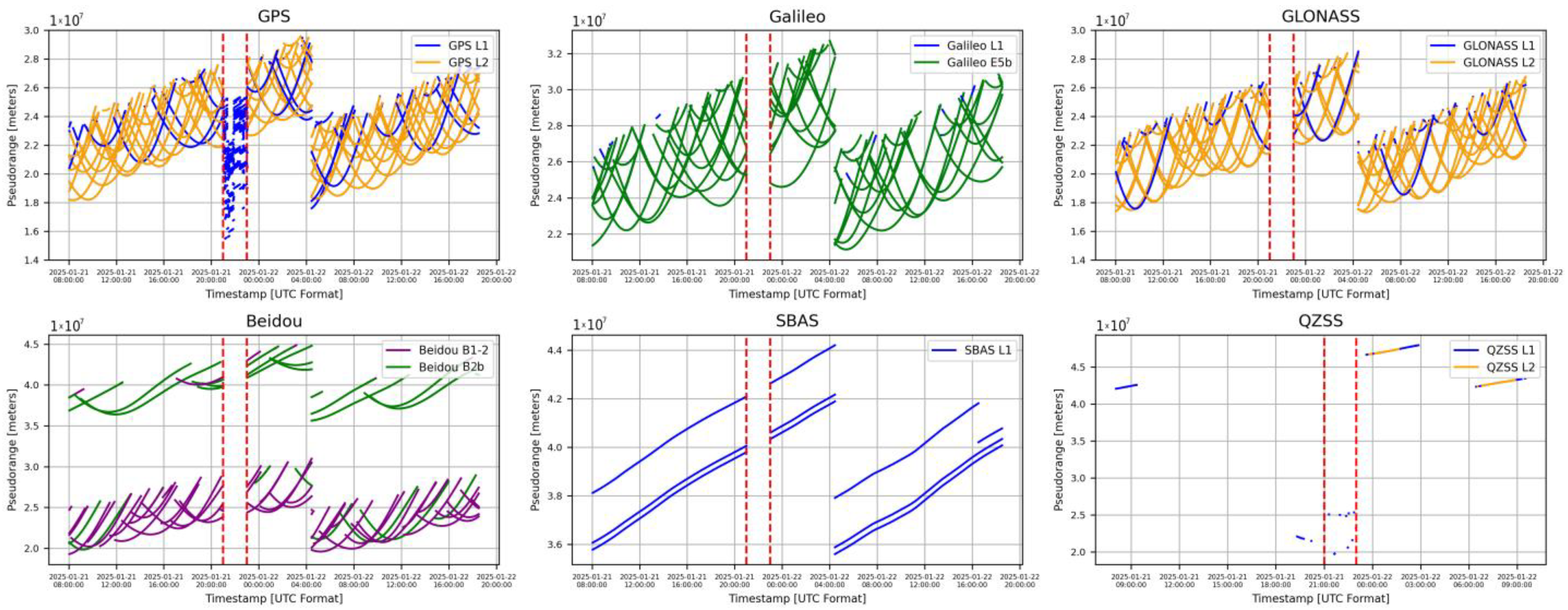
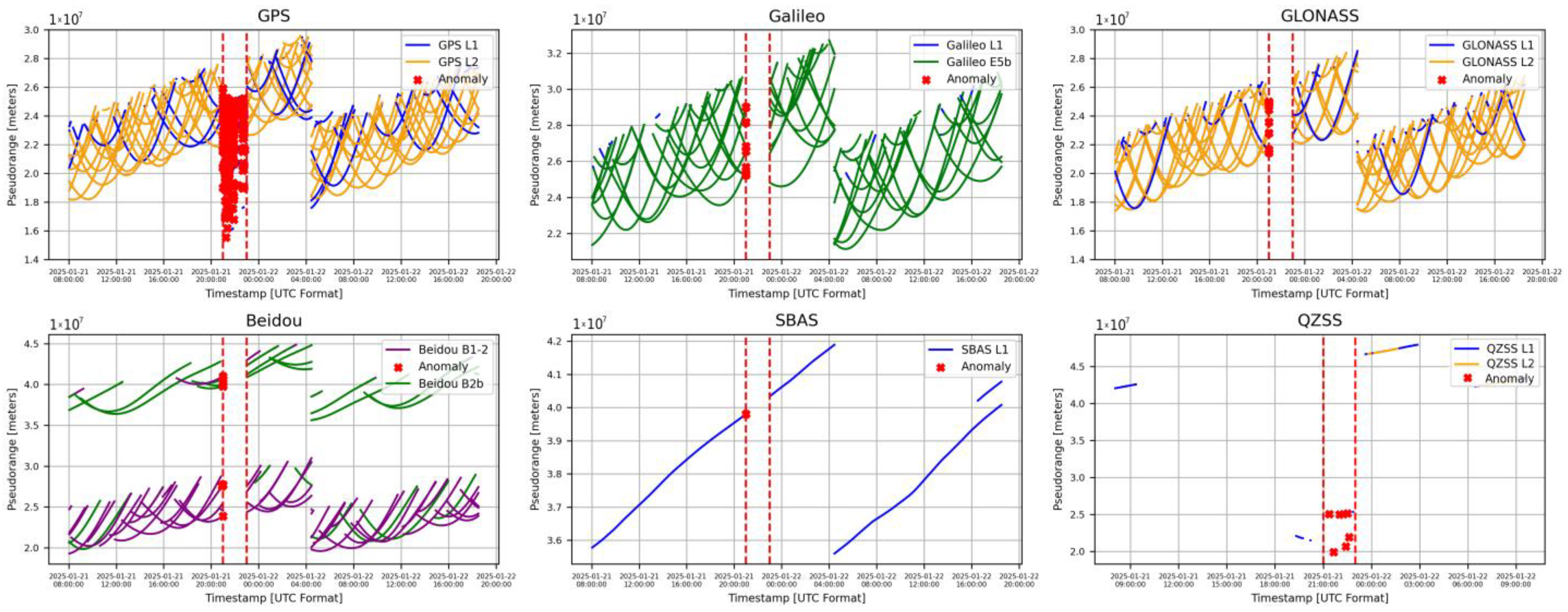
• Pseudorange Codes (Cxx): Denoted by C and followed by the band number and channel attribute, the parameter $R_P$ represents the measured distance $\rho$ between the receiver antenna and the satellite antenna, incorporating clock offsets $r_{clk offset}$ and $s_{clk offset}$ from both the receiver and satellite, as well as additional biases β such as atmospheric and propagation delays [32]. The parameter is expressed in meters and its calculation will take into account the speed of light. Based on these, the parameter can be expressed by the following relation:

  $$R_P=\rho +{\mathrm{c}}^{\ast } (r_{clk offset}-s_{clk offset})+\beta$$

  (1)
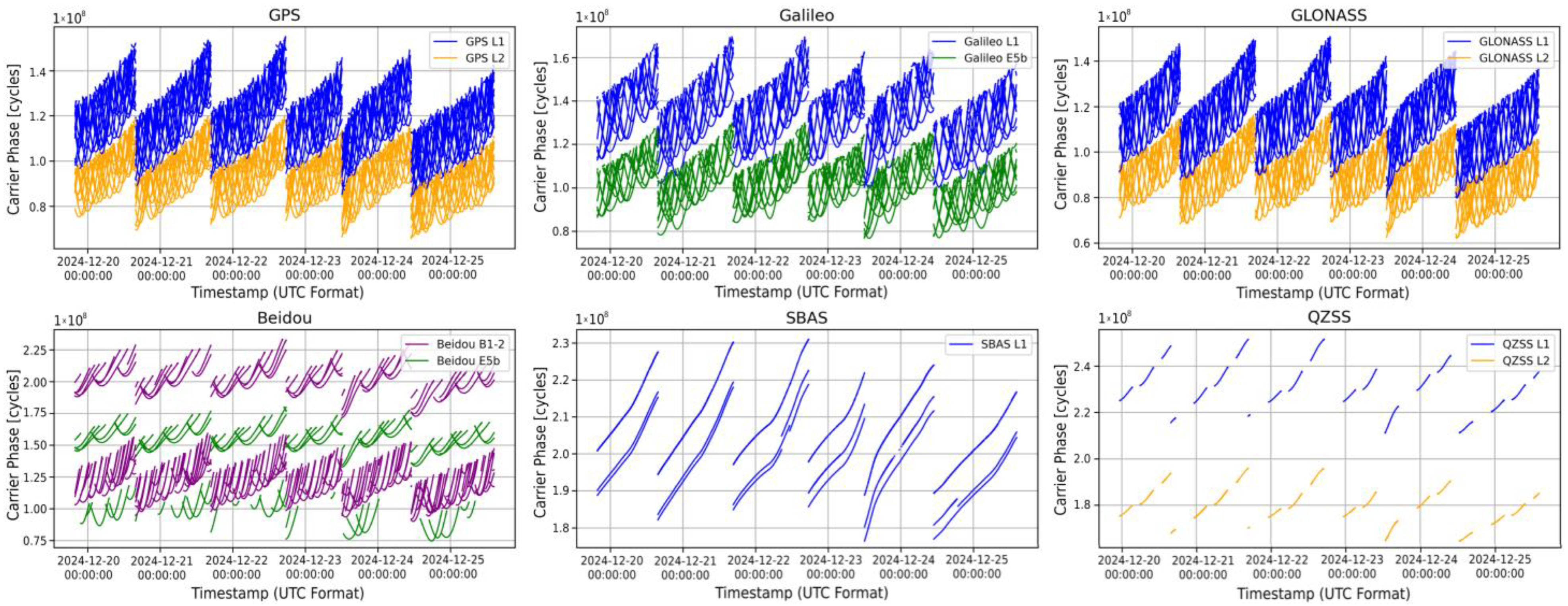
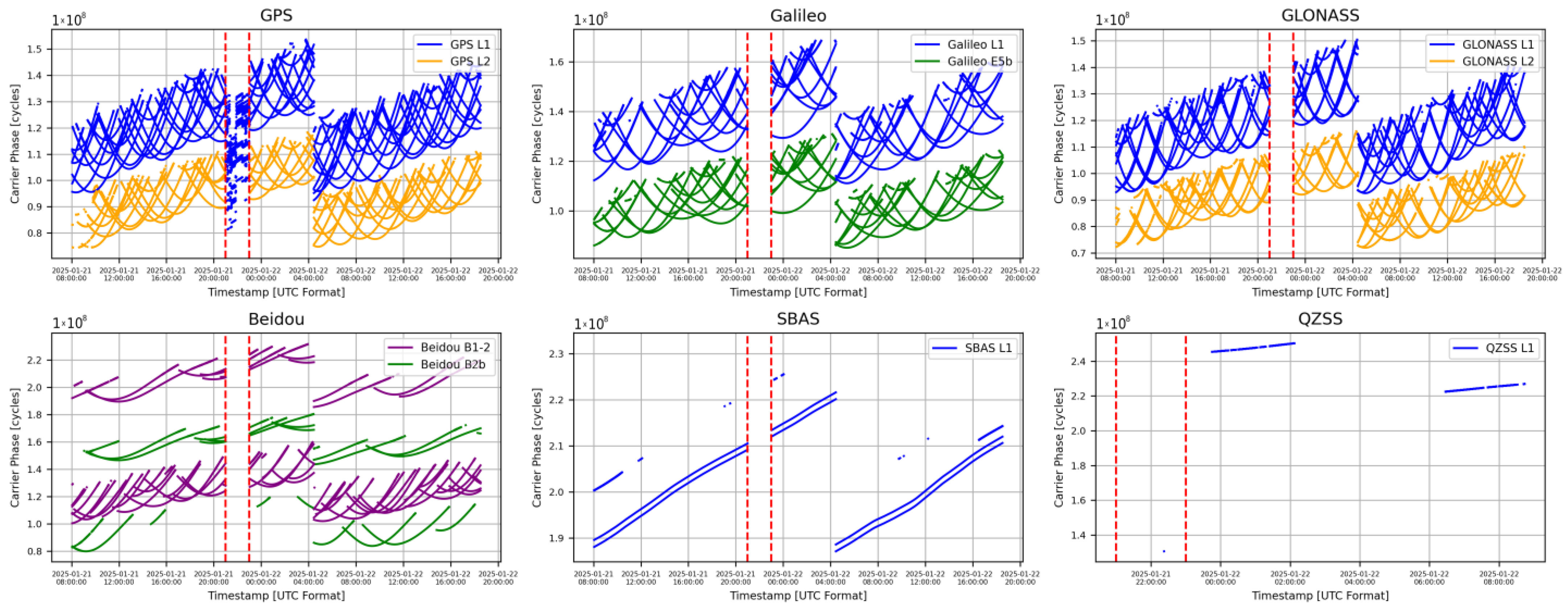
• Carrier Phase (Lxx): Denoted by L and followed by the band number and channel attribute, refers to the measurement of the accumulated phase of the carrier signal transmitted by a satellite, as received by a GNSS receiver.
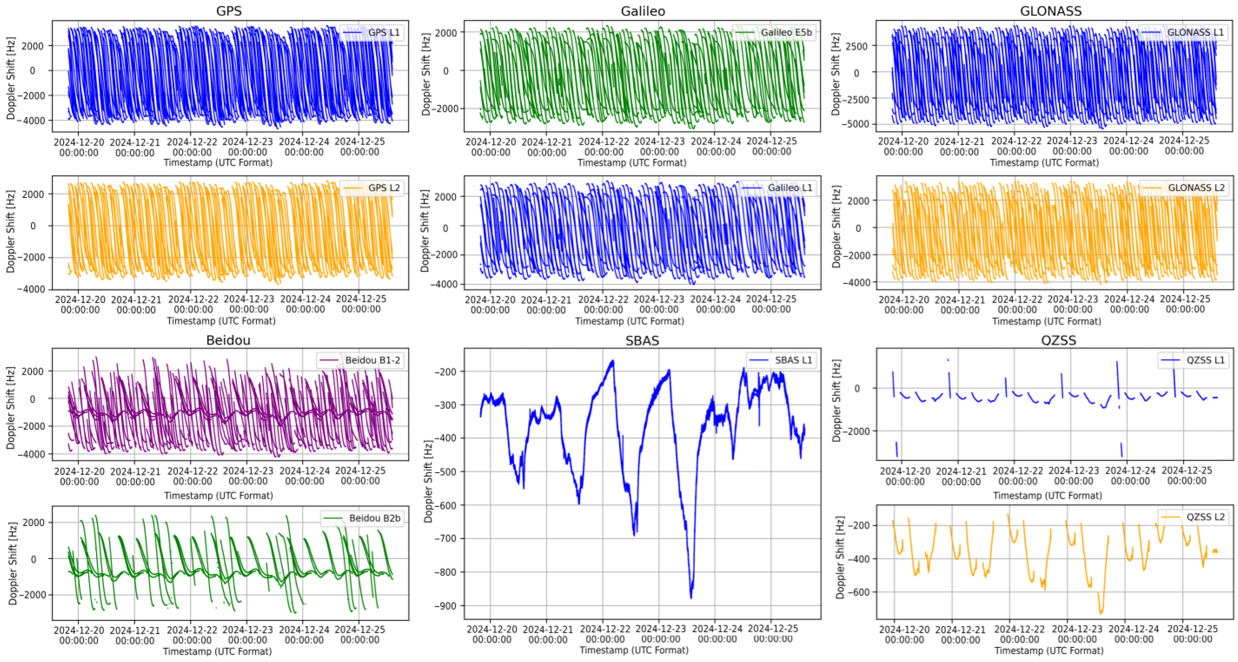
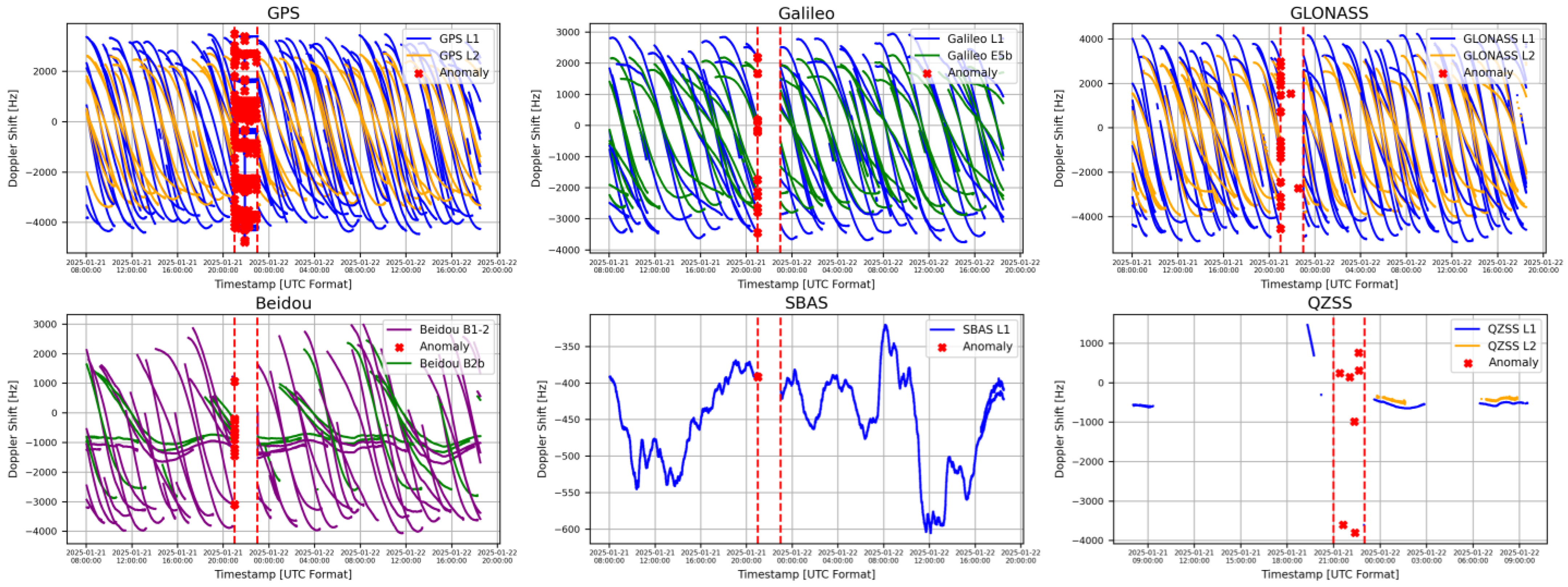
• Doppler Shift (Dxx): Denoted by D and followed by the band number and channel attribute, refers to the measurement of the frequency shift in the received satellite signal $f_R$ and transmitted satellite signal $f_T$ caused by the relative motion between the satellite and the receiver [33].

  $$∆f=f_R-f_T$$

  (2)
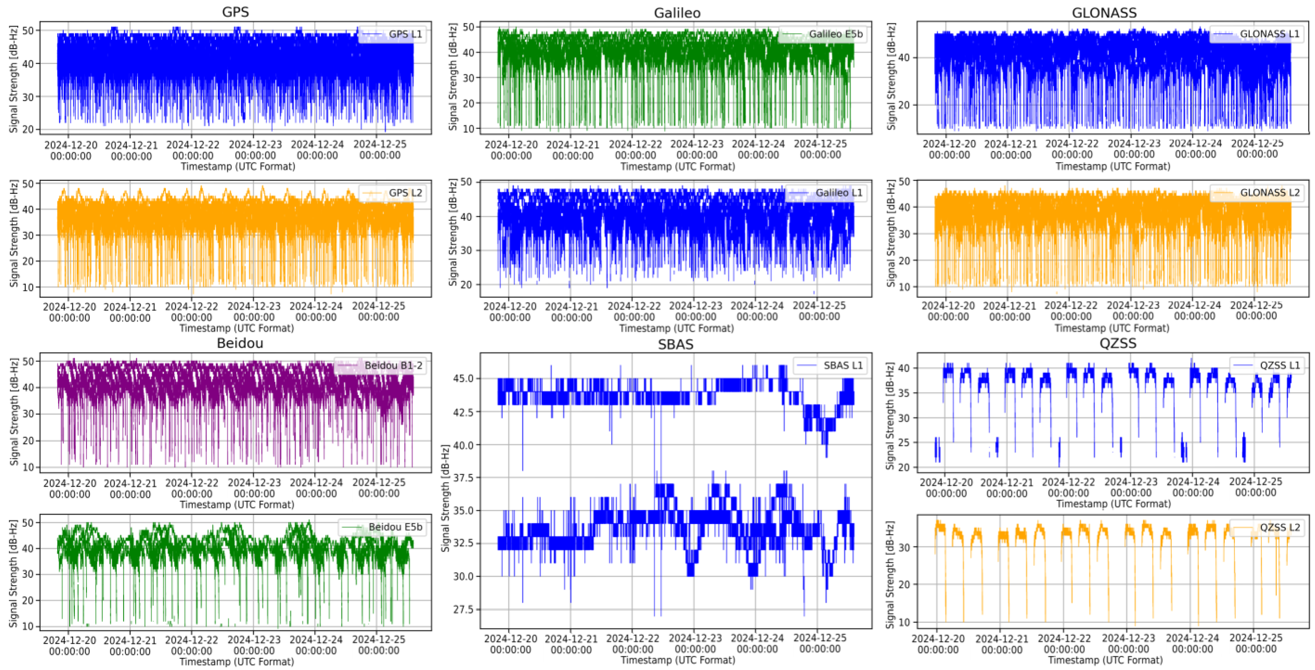
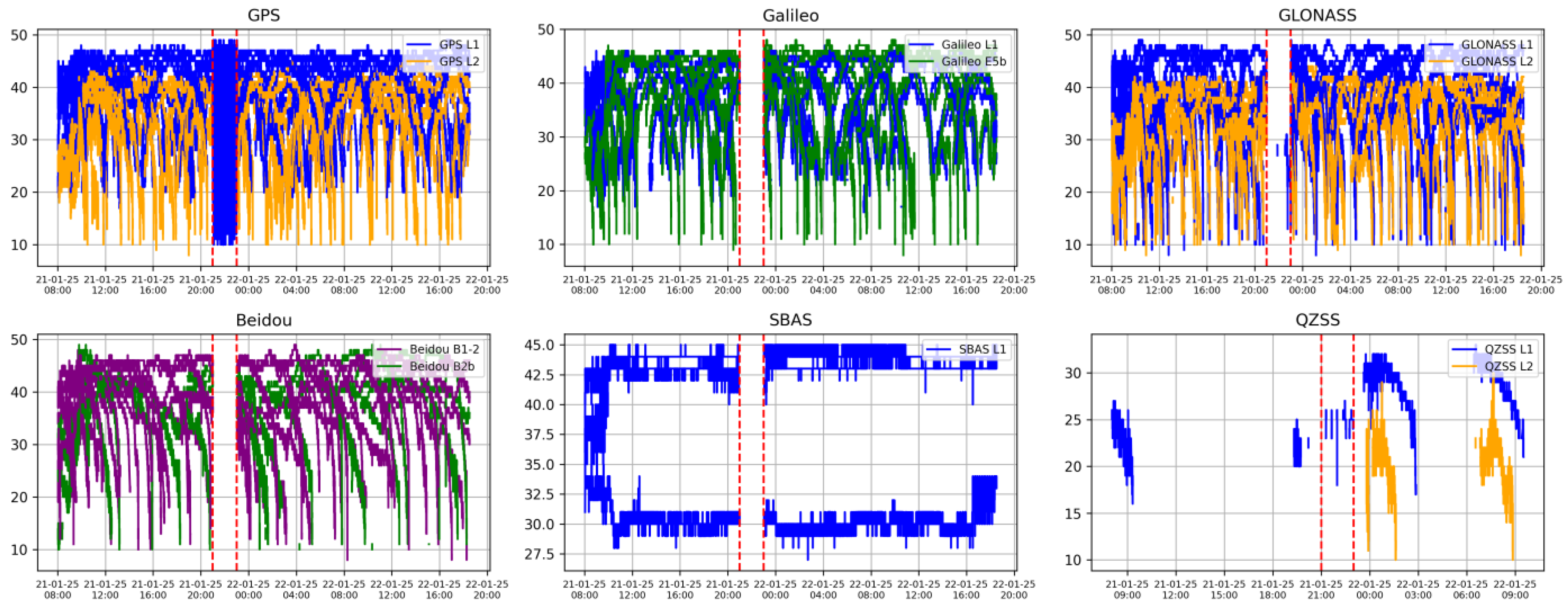
• Signal Strength (Sxx): Denoted by S and followed by the band number and channel attribute, refers to a measure of the power or quality of the received satellite signal at the receiver’s antenna [34]. In RINEX observation files, it is typically represented as Carrier-to-Noise Density Ratio (C/N₀) values, which indicate the ratio of the received signal power to the background noise level.

3. Literature Overview

To address the challenges posed by the increasing level of sophistication in the design and execution of GNSS spoofing attacks, there is a growing global effort within the academic and research communities to develop effective detection, mitigation, and security strategies to protect all GNSS users (smartphones, vehicles, airplanes, UAV/UAS, and so on). These efforts are focused on multiple complementary directions. One direction relies on traditional techniques, such as advanced signal processing methods and hardware-based countermeasures (e.g., antenna arrays). Some of these are tested and validated, in, e.g., [35,36,37], where experimental evaluations confirm the effectiveness of traditional spoofing countermeasures. A major limitation of these approaches is their dependency on large and specialized hardware components (e.g., signal analyzers, antenna arrays), which hinders seamless integration across the broad spectrum of GNSS user environments. A second line of research focuses on cryptographic and signal authentication mechanisms, including the use of navigation message authentication (NMA) and spread-spectrum encryption as shown in, e.g., [38,39]. These methods aim to ensure the authenticity and integrity of the transmitted signals and show a strong theoretical potential. Such techniques are still in the testing and validation phase, with limited availability in commercially deployed systems. A third and rapidly evolving direction, which will be our focus in this study, leverages data-driven approaches, particularly machine learning and deep learning techniques applied to data from different layers of the GNSS sensor architecture. Therefore, some recent research [23,40,41,42] tested machine learning-based methods (e.g., Support Vector Machine or Convolutional Neural Networks) for GNSS spoofing detection, using both simulated scenarios and real-world datasets. These methods achieved detection rates of up to 98.8% by leveraging supervised classifiers (e.g., SVM), ensemble models, and deep learning architectures such as CNNs, applied to statistical features. These recent methods and analyses have been tested on data with low temporal resolution, and an investigation using higher temporal resolution data is necessary.

To address our data with high temporal resolution, we employ a Long Short-Term Memory (LSTM)-based network to detect observation codes distortions generated by the attack. For instance, previous research [43,44,45,46] proposed advanced strategies for anomaly detection in multivariate and data-scarcity time series. In [43], the authors transform time series into images using Gramian Angular Fields and apply knowledge distillation-based image anomaly detection models. Their method, validated on benchmark datasets such as SWaT, UCR, and NAB, achieves F1-scores of up to 99%, showcasing high efficiency and accuracy. In [44], Lee et al. introduced an ensemble of multi-point LSTM predictors that forecast values at different time horizons and aggregate the results for anomaly detection. This approach is particularly relevant to GNSS signals, where multiple observation codes of each satellite signal can be analyzed through aggregation strategies. Further extending this direction, the authors from [47] presented a bilevel optimization framework (BiLO-Auto-TSF/ML) that integrates few-shot learning with hyperparameter tuning to improve forecasting under data scarcity. Compared to Auto-Sklearn 2.0, BiLO-Auto-TSF/ML-LSTM yields significantly better performance on wind energy data, with lower MSE (0.0247 vs. 0.0514) and improved SMAPE (35.79% vs. 39.65%). Similarly, [48] introduces a multioutput model capable of simultaneous imputation and forecasting by leveraging inter-task correlations, achieving superior results while reducing computational costs via kernel approximations. Complementing these technical advancements, [46] provides a comprehensive survey of deep learning-based methods for multivariate time series anomaly detection (MTSAD). The survey categorizes recent approaches into forecasting and reconstruction learning-based models and discusses their suitability depending on data characteristics and application goals.

Based on these, our work adapts LSTM-based anomaly detection to GNSS signal observation codes, with a focus on time-aligned measurements structured according to the RINEX standard. The proposed method leverages time series forecasting principles to identify anomalies indicative of spoofing attempts, thereby contributing an additional security layer within the GNSS.

4. Training and Testing Scenarios

In this section, we will present the systems and data used in the training and testing process of the LSTM algorithm. We will also realize the necessary configurations for the systems used in the training and testing processes.

4.1. Training Scenario and System Configurations

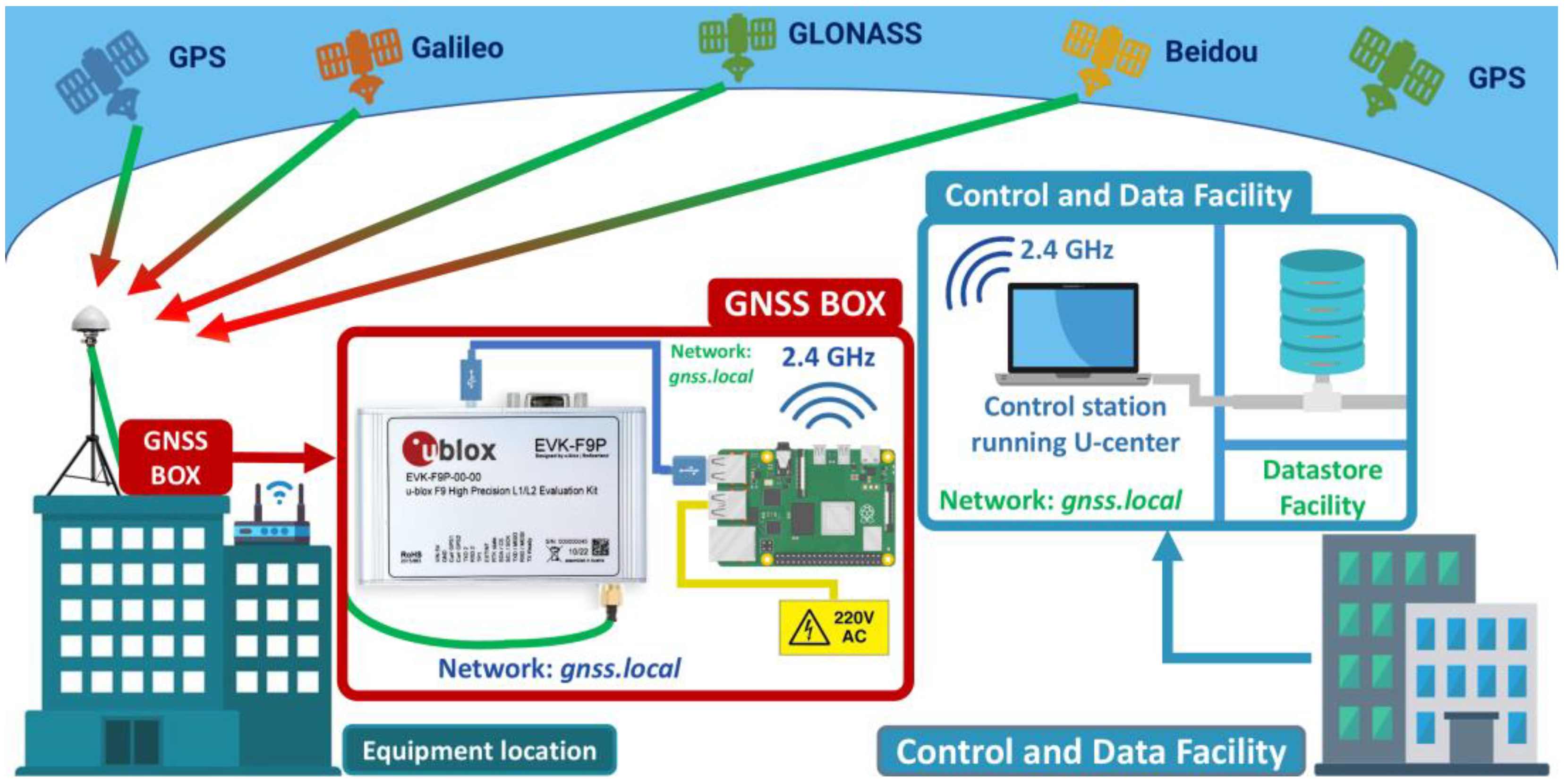
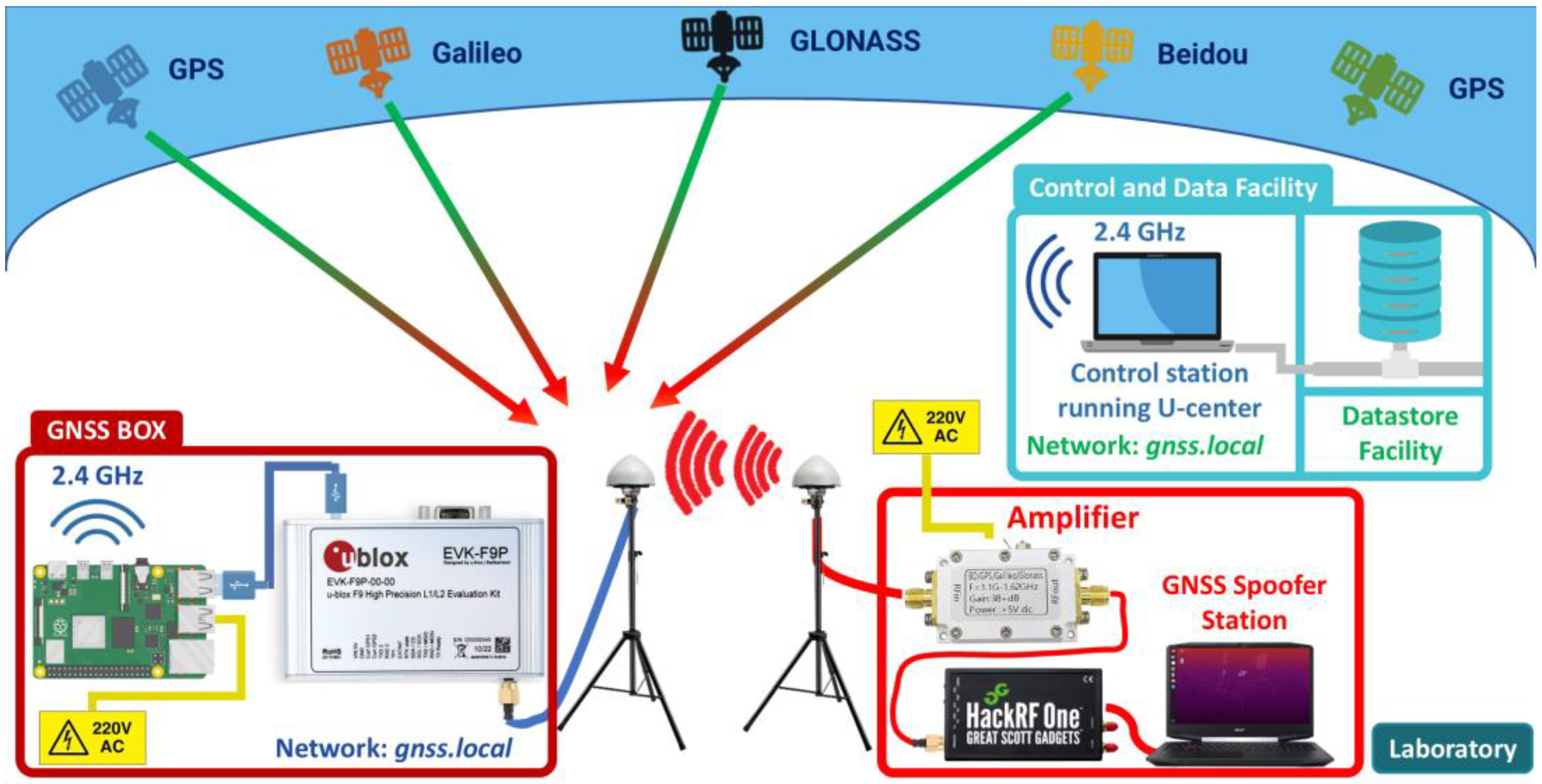
4.1.1. Training Scenario Topology

The data acquisition topology consists of a GNSS Box and a set of control and processing systems located in the Control and Data Facility. The GNSS Box is composed of a Raspberry Pi 4 Single Board Computer (SBC) (by Raspberry Pi Foundation, Cambridge, UK), a U-blox EVK-F9P GNSS sensor (by U-blox, Thalwil, Switzerland), and a multiband active GNSS antenna. The EVK-F9P module is a high-precision receiver compatible with multiple satellite constellations, including GPS, Galileo, GLONASS, Beidou, IRNSS, and QZSS, operating in the L1 and L2 frequency bands. To ensure optimal signal reception, the GNSS Box is installed on the rooftop of a 30 m high building to minimize interference from obstacles and multipath propagation. It is connected via a local Wi-Fi access point to the internal network gnss.local, enabling remote access. Within the Control and Data Facility, a Windows-based control station is connected to the same network and runs the U-Center 2 software version 24.09.118603 to manage remote acquisition and monitoring. The collected raw GNSS data are then transmitted and stored in a centralized Datastore server within the same network. Based on these, the proposed topology is illustrated in Figure 3 and will be used in training data acquisition.

To better illustrate the proposed topology, we can summarize it in a simple usage scenario as follows. The GNSS Box is installed on the rooftop of the university’s engineering building, providing clear sky visibility to minimize multipath effects. It operates continuously for a 48 h period, during which it receives signals from multiple GNSS constellations. The observation codes are collected using the U-blox EVK-F9P sensor (by U-blox, Thalwil, Switzerland) and streamed in real time via a local Wi-Fi access point. A control station located in the laboratory connects remotely to the GNSS Box using the U-Center utility to monitor and record raw GNSS data. The collected data are then stored in a centralized Datastore for preprocessing and used to train the LSTM model to learn normal signal patterns. Through this scenario, high-resolution GNSS data acquisition can be achieved.

4.1.2. System Configurations for Training Scenario

GNSS Box configuration involves the following steps:

• Libraries and dependencies installation: The libraries required to interact with the EVK-F9P sensor are gpsd, gpsd-clients, python3-gps, and ser2net. The gpsd daemon is used to manage the data received from the GNSS sensor and the gpsd-clients, python3-gps libraries are needed to interpret the navigation messages. The ser2net utility is required to establish TCP/UDP connections to the port assigned to the GNSS sensor by the Raspberry Pi operating system.

  sudo apt-get install gpsd gpsd-clients python3-gps ser2net
• Configuring GNSS sensor remote data transfer:
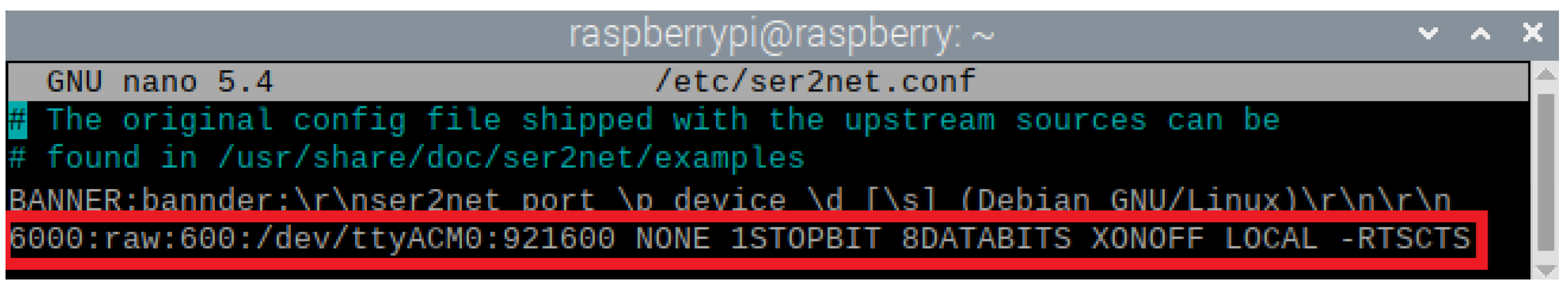
  • GNSS sensor assigned port query: To perform remote data transfer, it is necessary to query the port assigned by the operating system. The port allocated to the GNSS sensor by the operating system will be a teletype (tty) port, usually ttyACM0 port.

    sudo ls/dev/tty*
  • Ser2net configuration: The tty port must be set in the ser2net config file, through which a TCP connection on port 6000 at a 921,600 bitrate will be established. Figure 4 shows the ser2net configuration file, as well as the command used to configure the TCP connection to the teletype port ACM0.

Through the configured settings, the GNSS Box has a TCP port 6000 open for data transfer from the serial port ttyACM0. Next, the remote connection will be tested using the U-center application installed on the control station. The U-center application is developed by U-blox, the manufacturer of the sensor, and is a tool that enables real-time graphical representations of the navigation data from the sensor. In addition, the application allows for storing sensor data via remote connections. To achieve this, the IPv4 address of the GNSS Box station assigned by the Wireless AP is required. In our case, the IPv4 address is 172.31.10.20 with TCP port 6000. Next, as shown in Figure 5, the connection is active, and the application is receiving navigation data from the GNSS Box.

From the Message View menu, it is necessary to enable the messages and data that the application will store. In our case, the messages of interest for the RINEX standard are UBX and RXM-RAWX. These messages are specific standards for GNSS and contain raw navigation data received from the sensor. The recorded data are saved in raw format in files with .uc2 and .ubx extensions. After the data acquisition period, it is necessary to convert these files using special conversion tools such as RTK Library version 2.4.3_b34.

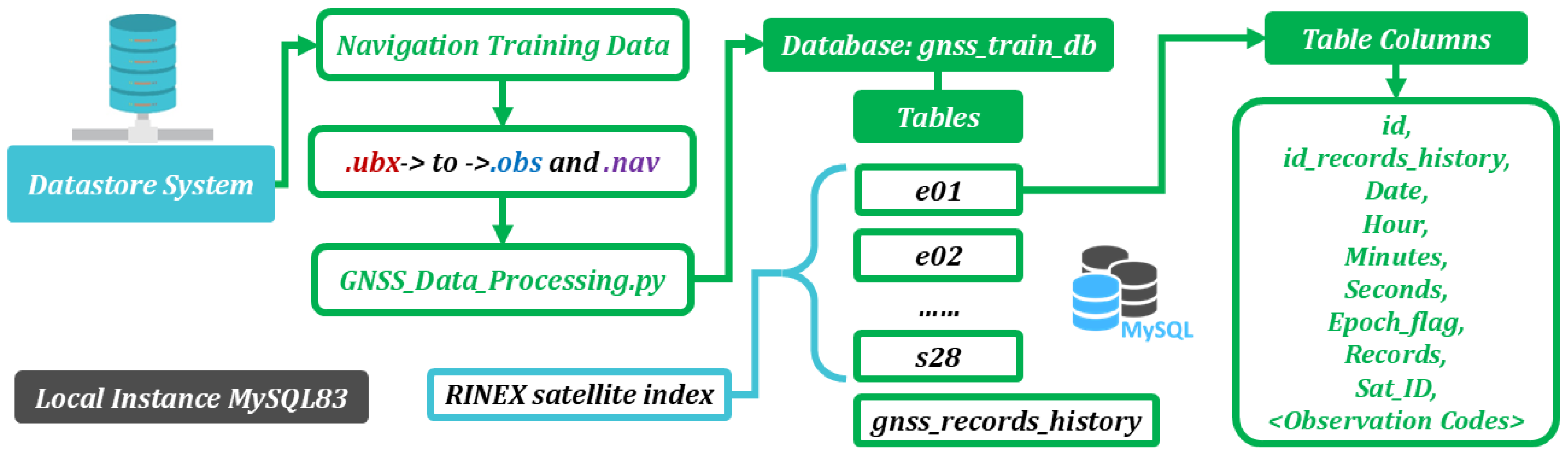
4.1.3. Training Data Processing

Model training requires a sufficiently large volume of data to capture the pattern of navigation signal observation codes for each satellite. Therefore, starting from the fact that the orbital period of the navigation constellation satellites varies between 12 and 24 h, we set the training data acquisition period to 7 days between 19 December 2024/19:47 and 25 December 2024/19:53 UTC time. After this period, the U-center application generated two files: one with the .uc2 extension and another with the .ubx extension. The information in these files is in raw format. Therefore, the RTKLib utility will be used to convert them into RINEX. Next, the conversion process using RTKLib is illustrated in Figure 6.

The resulting .obs file generated by the RTKLib utility contains over 250 million rows, making it extremely difficult to open with standard programs. Therefore, we decided to use MySQL databases to store the .obs file data in a structured and easily accessible format. Within the .obs files, the observation codes for each satellite are recorded within the measurement epochs. Each epoch is identified by “< Date Month Day Hour Minutes Seconds Epoch_flag Number_of_Satellites”, as shown in Figure 7.

The epoch identifier is followed by rows with the observation code measurements for the satellites of that epoch. The rows consist of the satellite identification code (first column) and the following columns contain the observation code values for the satellite. Thus, in order to identify which observation code the values belong to, a mapping is realized between the satellite identification code and the observation codes in the header marked with the SYS/#/OBS TYPES tag. Based on these, the data processing, filtering, and centralized storage workflow will be implemented using a Python script version 3.13 which is illustrated in Figure 8 and described in Algorithm 1.

Algorithm 1. GNSS Data Processing

1: DATABASE Open Connection

2: OPEN .obs file

3: READ .obs file Header to get <Observation Codes>

4: for line in file.lines

5: if line.startwith(‘>’)

6:   EXTRACT Epoch_info = [Date, Hour, Minutes, Seconds, Epoch_flag, Records]

7: else

8:   EXTRACT Sat_ID, <Observation Codes Values>

9:   if Sat_ID.table.exists == False

10:    CREATE Sat_ID.table with columns [Epoch_info, <Observation Codes>]

11:   STORE [Epoch_info, <Observation Codes Values>] in Sat_ID.table

12: end for

13: DATABASE Close Connection

The Python script from the data processing workflow reads the .obs file, identifies each epoch through “>” sign, and retains the epoch information (Year Month Day Hour Minutes Seconds Epoch_flag Records) and the satellites in that epoch. Then, for each satellite identified in the epoch, it generates a table in the gnss_train_db database with the name of the satellite. After this step, the script generates the following columns in each table: id; id_records_history; Date = Year-Month-Day, Hour, Minutes, Seconds; Epoch_flag; Records; and Sat_ID. Following the Sat_ID column, the script creates additional columns named after the satellite’s observation codes, based on the “SYS/#/OBS TYPES” tag from the RINEX header. Then, a repetitive “for” loop iterates through each line of the file and stores the values from each column into the corresponding satellite table. The Python script is presented in the table below.

4.2. Testing Scenario and System Configurations

4.2.1. Testing Scenario Topology

The testing scenario involved using a dataset acquired by exposing the GNSS sensor to false navigation signal emissions. By exposing the sensor to these signals, we captured its behavior under real spoofing conditions. The GNSS sensor used was the same GNSS Box station as in the training scenario, while the spoofed signal emissions were generated using a system based on SDR solutions. Data acquisition for this scenario was performed in a controlled environment, as the emission of such GNSS signals is strictly regulated. The systems used in this scenario are illustrated in Figure 9 and include the GNSS Box, an emission station that carried out the spoofing, and a control station for data acquisition. The spoofing station, referred to as the GNSS Spoofer Station, consisted of a laptop (by ASUSTeK Computer Inc., Taipei, Taiwan) running Ubuntu OS (by Canonical Ltd., London, UK), an SDR model HackRF One (by Great Scott Gadgets, Denver, CO, USA), and a signal amplifier.

4.2.2. System Configurations for Testing Scenario

For this scenario, the GNSS Box system and control station have the same configurations as those used in the training data acquisition. Regarding the GNSS Spoofer Station, additional configurations are required to enable signal transmissions.

GNSS Spoofer configuration involves the following steps:

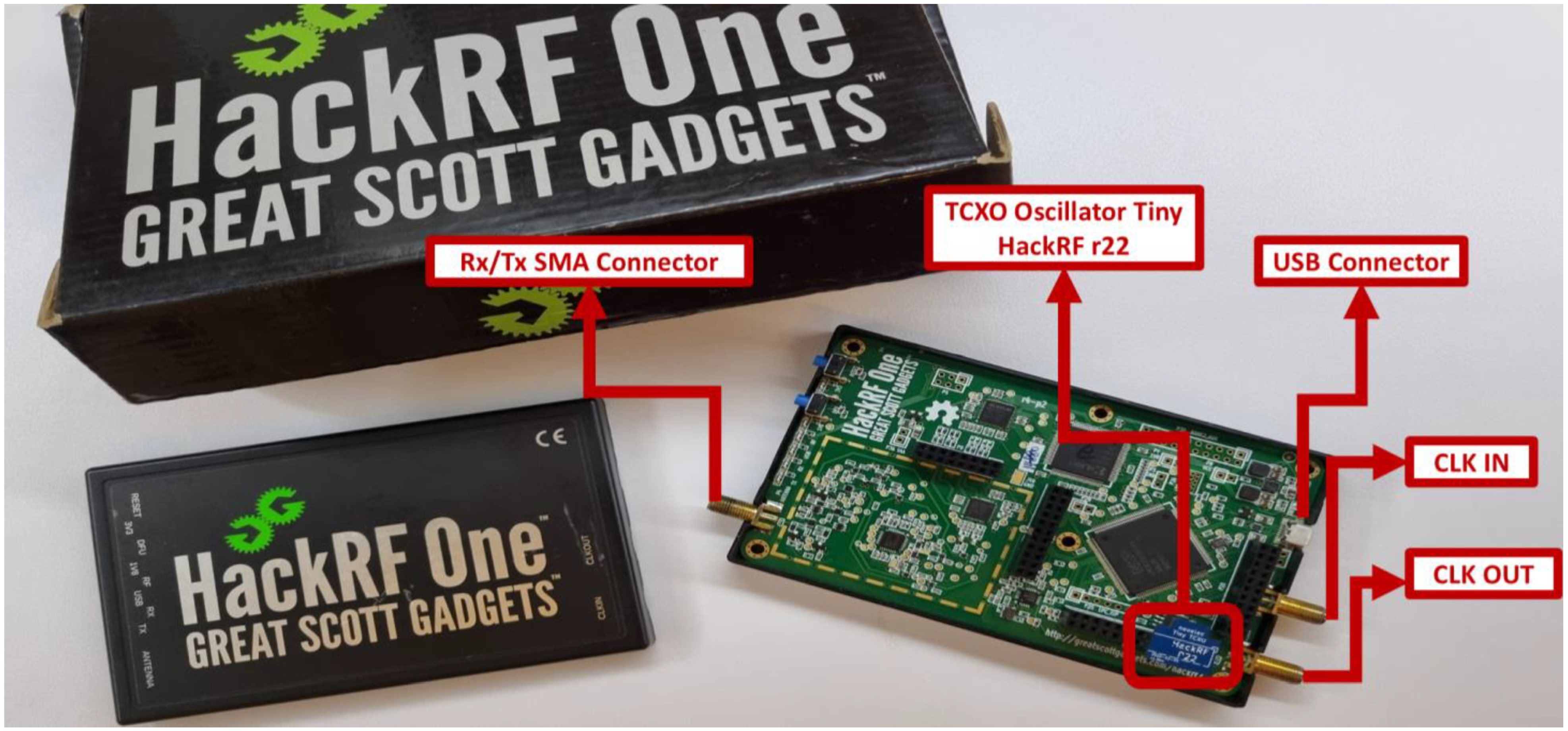
• HackRF One installation: The device is an SDR solution that allows transmission and reception of radio signals over a wide frequency range (1–6 GHz). To use HackRF One for GNSS spoofing, it requires proper driver installation and firmware updates.

  sudo apt-get install hackrf
• TCXO installation: It is recommended that the GNSS signal transmission using HackRF be performed with the aid of a frequency stabilizer to ensure signal accuracy. This can be achieved by using a Temperature Compensated Crystal Oscillator (TCXO), which minimizes frequency drift caused by temperature variations and ensures a more precise and stable signal [49]. The oscillator used is a Nooeiec model and was inserted into the port P22 on the board, as shown in Figure 10. Once the oscillator is inserted, we need to check that the TCXO is recognized by the device. If the following command output is [0] = 0 × 51, then the oscillator is not recognized and if the output is [0] − 0 × 01, then the oscillator is successfully recognized.

  hackrf_debug-–si5351c-n 0-r
• GNSS Spoofing Application development: The application that will perform the generation of the false navigation signal sample was developed using the Python programming language and open-source libraries. Next, the application will perform the following operations:
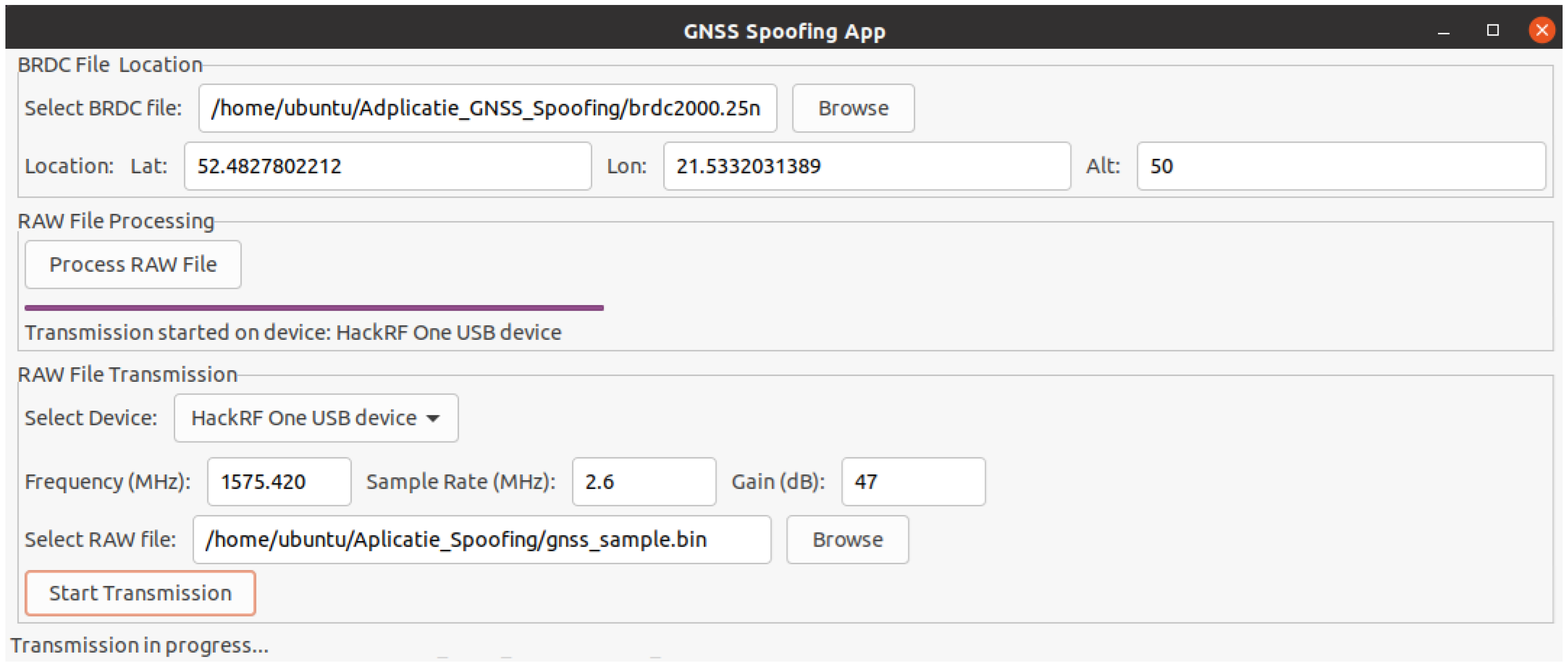
  • Signal sample generation: Acquiring a navigation signal sample can be accomplished by several methods. The first method is to record the navigation signals and output them at a later date. The second method is to generate the signal using its specific data and technical parameters. In our scenario, the second method was used in the development of the application due to the fact that it allows greater control over the navigation data. In the following, for signal sample generation, we used the structure and technical specifications of GPS signals in the L1 band, as this is one of the main bands used in navigation. Generating a navigation signal sample for a specific system involves the use of its ephemeride files. These files contain precise orbital and clock data of the satellites, allowing accurate reconstruction of satellite positions and navigation data [50]. For the GPS constellation, ephemeride files can be obtained online from the Crustal Dynamics Data Information System (CDDIS). In our scenario, we have used the ephemerides file corresponding to 21 January 2025, i.e., the file brdc2000.25n. Next, the process of generating signal samples using the chosen ephemerides file is realized using a series of libraries developed by Takuji Ebinuma and his collaborators from the gps-sdr-sim project, available on the GitHub platform. These libraries are getopt.c, getopt.h, gpssim.c, gpssim.h, gpssim.o, which we have integrated in our application. These libraries will help to extract the satellites from the ephemerides file corresponding to a given location (latitude, longitude, and altitude) and to generate the raw navigation data file.
  • Signal sample transmission: After generating the raw navigation data file, its transmission will be realized using the hackrf_transfer.c module from the installed hackrf library. This module allows us to set the transmission frequency, sample rate, gain, and many other options at which the signal sample will be transmitted. Figure 11 shows the interface of the application built using Python version 3.13 that will realize the signal sample generation and transmission.

In generating the sample signal, the location determined by latitude 52.4827802212, longitude 21.5332031389, and altitude of 50 m was used. These dates correspond to the location of Sitne in Poland, which was chosen at random. Also, the transmission frequency is 1575.42 MHz with a sample rate of 2.6 MHz and a gain of 47 dB.

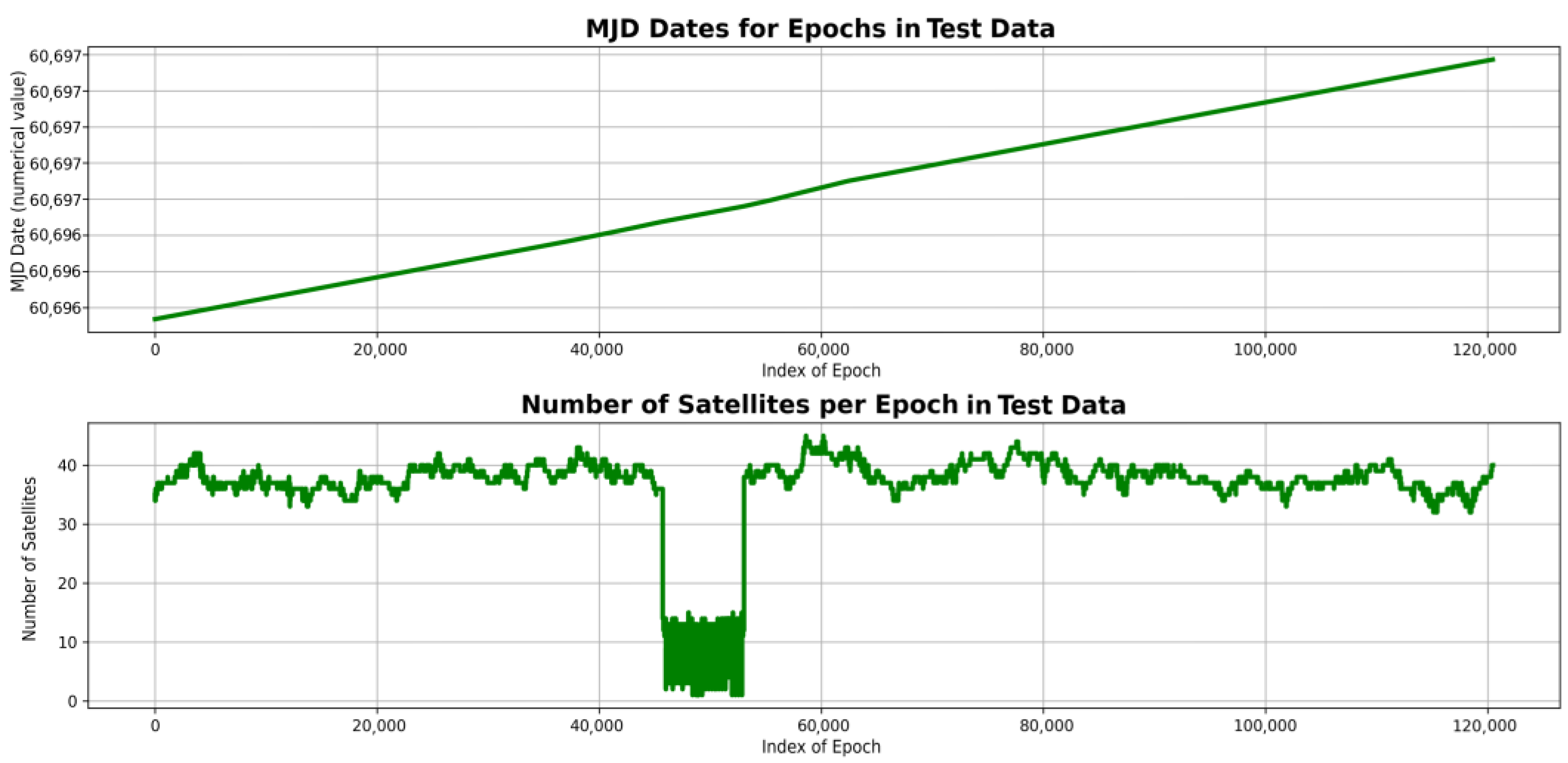
4.2.3. Testing Data Processing

The test data acquisition using the systems and application presented above was performed for 24 h on 21 January 2025. The signal sample emission generated by the application on the GNSS spoofing station was turned on for 2 h in the time interval 21:00–23:00 on the same day. During the 24 h, the control station recorded the data transmitted by the GNSS Box. Using the same procedure as that used to collect and process the training data, the resulting data were converted into observation files and then stored using Algorithm 1 in a database called gnss_test_db.

5. Results and Discussion

In this section, we present the architecture of the LSTM model used in the training and testing process based on the data acquired in the previous sections. Additionally, we described the training and testing datasets, as well as the attack detection method implemented within the algorithm.

5.1. LSTM Architecture and Training Results

5.1.1. LSTM Training Architecture

The LSTM model architecture for the training process is based on TensorFlow/Keras, NumPy, Pandas, Scikit-learn, and SQLAlchemy libraries. The training data are taken from the MySQL database called gnss_train_db, where each table corresponds to a satellite and where the observation codes are stored in columns. Next, the model operates in a multi-feature setting, where the input sequence is constructed from all four observation codes associated with satellite signals (e.g., CxI, LxI, DxI, SxI). These features are treated as a multivariate time series of dimension 4. The objective is to train the LSTM model to reconstruct these sequences, thereby capturing the joint temporal dependencies across features. To systematically evaluate the impact of architectural choices and training parameters, we implemented an automated hyperparameter tuning strategy using Optuna, a modern framework for efficient and reproducible search across parameter spaces. The system explores combinations of number of layers [2, 4]; loss function [MAE]; learning rate [10⁻⁴]; latent dimensions [8, 16, 32, 64]; dropout [0, 0.2, 0.4]. In addition, the data are normalized using Standard-Scaler and subsequently split into 80% for training and 20% for validation, ensuring a well-balanced learning process. The LSTM model architecture is symmetric, consisting of an encoder–decoder structure designed to reconstruct the entire multivariate input sequence. The training is performed over 50 epochs with a fixed batch size of 1024, which offers a good balance between convergence stability and computational efficiency. Each configuration was evaluated automatically and in parallel across observation codes of each satellite signal using the multiprocessing library. A subset of configurations was selected and is summarized in

Table 1. LSTM hyperparameter tuning.

No.	Model Configuration	Dropout	Learn. Rate	Layers	Latent_DIM	Loss Function	MAE	RMSE
#1	Complete model	0.2	1.00 × 10−4	4	16	MAE	0.117	0.186
#2	No dropout	x	1.00 × 10−4	4	16	MAE	0.162	0.25
#3	Simplified	0.2	1.00 × 10−4	2	16	MAE	0.169	0.256
#4	Latent_DIM = 8	0.2	1.00 × 10−4	4	8	MAE	0.138	0.215
#5	Latent_DIM = 64	0.2	1.00 × 10−4	4	64	MAE	0.132	0.199
#6	Dropout = 0.4	0.4	1.00 × 10−4	4	16	MAE	0.141	0.22

.

The models configured in the table illustrate how specific architectural choices affect model performance. Based on the validation MAE and RMSE values, configuration 1 was selected as the optimal setup for out data, offering a strong balance between generalization capability and computational cost. Also, the main structure of the training code is presented in the pseudocode Algorithm 2 below where model configuration 1 was configured.

Algorithm 2. LSTM Training from DB

1: DATABASE Open Connection (gnss_train_db)

2:  GET list of tables (satellites), excluding gnss_records_history table

3: for table in tables.gnss_train_db

4:  LOAD data.table into Pandas DataFrame

5:  GET timestamp = [Date, Hour, Minutes, Seconds]

6:   CONVERT into a DateTime column

7:  GET set of <Observation Codes> for each satellite signal

8:  for each set of <Observation Codes>

9:     LOAD Observation_Code.values

10:   CLEAN Observation_Code.values for NaNs

11:   NORMALIZE StandardScaler(<Observation_Code.values>)

12:   SPLIT data into 80% training and 20% validation

13:   BUILD LSTM model

14:    Input: n_features = 4

15:    Encoder: LSTM(64) -> Dropout(0.2) -> LSTM(32)

16:    Bottleneck: RepeatVector(16)

17:    Decoder: LSTM(32) -> Dropout(0.2) -> LSTM(64)

18:    Output: TimeDistributed(Dense(4))

19:    Compile: Adam Optimizer and MSE Loss Function

20:   TRAIN LSTM model

21:    Fit Model: Early Stopping—Monitoring Validation Loss

22:   SAVE trained model (Keras format)

23:  end for

24: end for

25: DATABASE Close Connection

5.1.2. LSTM Training Data

An overview of the dataset used for model training is presented in

Table 2. Training data overview.

Description	Values
Measurement period	2024-12-19T19:47:00–2024-12-25T19:53:00
Total number of observed satellites	127 satellites (Beidou-36, Galileo-25, GPS-32, GLONASS-24, QZSS-6, SBAS-4)
Total number of recorded epochs	500,000
Total number of recorded observations	19,966,505
Measurement location	Romania

, which includes key information such as the measurement period, the total number of observed satellites, the total number of recorded epochs, the total number of GNSS observations, and the measurement location. This summary provides context regarding the volume, diversity, and spatial–temporal characteristics of the data used to train and evaluate the LSTM-based reconstruction models.

A verification that the measurements and conversion process were performed correctly can be carried out by analyzing the Modified Julian Date (MJD) and the number of satellites recorded in the RINEX files. The MJD parameter represents a continuous count of days since midnight UTC on 17 November 1858. This parameter is extracted from the header of each epoch in the RINEX file. In Figure 12, it can be seen that the upward trend of the MJD parameter indicates a continuous and sequential increase in observation epochs, which is consistent with the expected time evolution in the RINEX file. Regarding the number of satellites within the visibility range of the sensor at each epoch among the 500,000 recorded epochs, it fluctuates between 33 and 49 satellites. This variation is expected due to the dynamic nature of satellite orbits, atmospheric conditions, and potential obstructions that may affect GNSS signal reception.

The first parameter used in LSTM training is Pseudorange. Figure 13 shows a representation of this parameter for GPS, Galileo, GLONASS, Beidou, SBAS, and QZSS, respectively, for the Pseudorange observation codes in the L1, L2, E5b, B1-2, and B2b frequency bands. The parameter is represented in meters and the time interval is in dd-mm-yy/hh:mm format. For the GPS, Galileo, GLONASS, and Beidou systems, it can be seen that the parameter plots overlap almost perfectly for the majority of satellites. This is because a satellite can transmit navigation signals in one or more frequency bands.

The next parameter used in training is Carrier Phase and Figure 14 provides a representation of it. Carrier Phase represents the accumulated phase of the GNSS signal’s carrier wave as received by the sensor [51]. It is measured in cycles and provides high-precision positioning information when combined with Pseudorange. In our data, it can be seen that there is a difference between the Carrier Phase of the L1 and L2 bands. This difference is normal because the parameter is measured in carrier wave cycles and the wavelength is different for each frequency band. For SBAS and QZSS, the parameter behaves differently due to the geostationary satellites of these constellations.

The next parameter is Doppler Shift and represents the rate of change in the frequency of the received GNSS signal due to the relative motion between the satellite and the receiver. In Figure 15, the parameter value is expressed in Hz and in GNSS spoofing detection, abnormal variations can indicate signal.

This effect is caused by the Doppler Shift, which occurs when a signal source (satellite) is moving relative to the observer (receiver). Usually, a positive Doppler value indicates that the satellite is moving toward the receiver, causing an increase in the received frequency. On the other hand, a negative value indicates that the satellite is moving away from the receiver, causing a decrease in frequency. In spoofing attacks, the station transmitting false navigation signals is typically static in most scenarios. As a result, the parameter value and pattern will undergo significant changes, deviating from the expected variations in the legitimate signals.

The last parameter used in LSTM training is Signal Strength, which is related to the Carrier-to-Noise Density Ratio (C/N₀) and represents the quality and strength of the received GNSS signal [52,53]. Figure 16 provides a representation of it for each constellation.

The parameter is typically expressed in dB-Hz and provides an indication of how strong and reliable the received GNSS signal is relative to background noise [51]. Higher parameter values indicate a stronger and more reliable signal, typically when the satellite is at a high elevation and with minimal interference. Lower parameter values may indicate signal degradation due to multipath effects, atmospheric disturbances, obstructions (buildings, trees), or other interference. Abrupt fluctuations in this parameter can be an indicator of GNSS spoofing, as artificially generated signals may have different power characteristics compared to authentic satellite signals. Under normal conditions, GNSS satellites transmit weak signals that undergo significant attenuation as they travel through the atmosphere. Spoofers, on the other hand, transmit stronger signals to override the legitimate satellite signals. This results in abnormally high Signal Strength values that can be detected and associated with an attack.

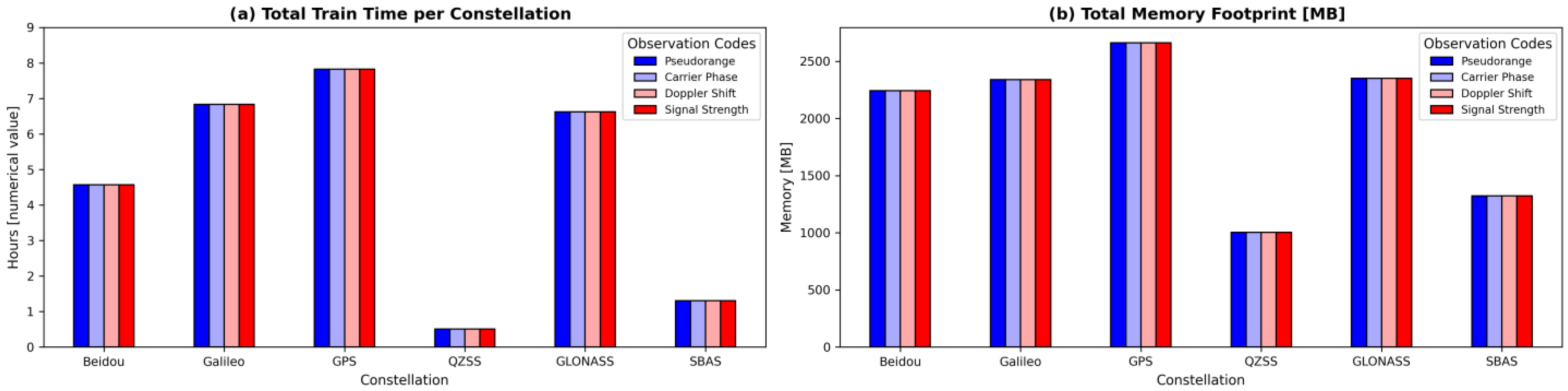
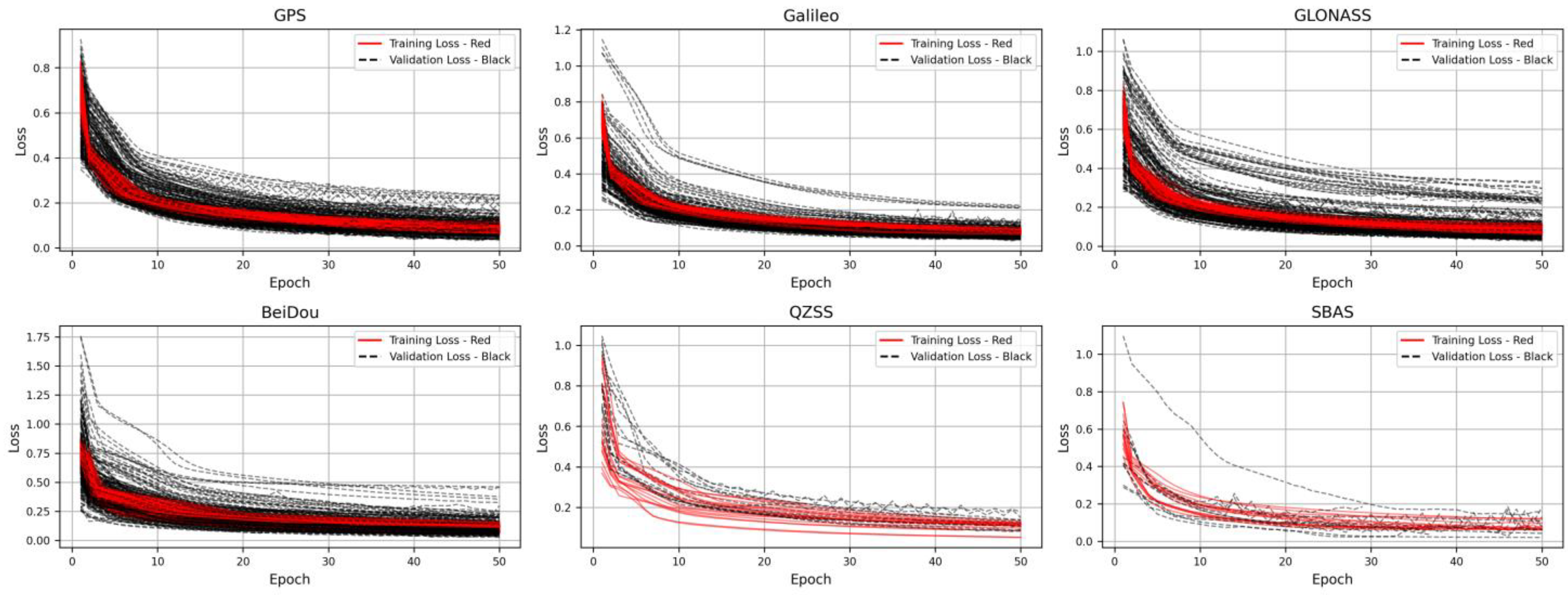
5.1.3. LSTM Training Performances

Based on the setup architecture selected above, the training performance of the LSTM models was assessed in terms of computational cost across different GNSS constellations and observation code types. Figure 17 illustrates two key metrics, (a) the total training time per constellation (in hours) and (b) the total memory footprint (in MB), consumed during model training.

As shown in Figure 17a, the GPS constellation required the highest cumulative training time, with values exceeding 8 h for each signal. Galileo and GLONASS follow closely with training times around 7 h. In contrast, QZSS and SBAS involved significantly shorter training durations, reflecting the lower volume of observation data available for those systems. Figure 17b highlights the corresponding memory usage during training, with GPS again exhibiting the highest memory footprint, surpassing 2500 MB. Other constellations such as BeiDou, Galileo, and GLONASS remain consistent within the 2100–2300 MB range, while QZSS and SBAS maintain lower memory demands.

Next, Figure 18 presents the evolution of training loss (in red) and validation loss (in black dashed lines) for the satellite signals corresponding to each GNSS constellation. The plots summarize the model convergence over 50 epochs across all observation codes used in training.

For all constellations, the LSTM models exhibit a rapid decrease in loss during the initial epochs, followed by a stable convergence phase, typically after epoch 20. The training and validation losses follow closely, indicating good generalization and low overfitting. In the cases of QZSS and SBAS, although the training curves also converge, the validation loss curves show higher variability. This is especially visible for SBAS, where several validation curves remain relatively flat or diverge slightly after epoch 20.

5.2. LSTM Architecture and Testing Results

5.2.1. LSTM Testing Architecture

The testing process is based on the test data collected during the attack and LSTM models trained on legitimate data. The testing data are taken from the MySQL database called gnss_test_db, which has the same structure as the training database. After establishing the database connection, the testing code iterates through each satellite table. For each signal group, the script loads the corresponding set of four observation codes. Missing values are removed, and the data are normalized using the same StandardScaler instance applied during training. The trained LSTM model associated with that signal is then loaded, and the reconstruction of the input sequence is computed. For each sequence, the reconstruction error is calculated as the mean absolute error (MAE) between the original and the reconstructed sequence. To detect potential anomalies associated with spoofing attacks, a threshold thr is applied. This threshold is computed based on the sigma rule:

$$\mathrm{thr}={\mu }_{\epsilon }+k\ast {\sigma }_{\epsilon }$$

(3)

where ${\mu }_{\epsilon }$ = mean of the reconstruction errors; ${\sigma }_{\epsilon }$ = standard deviation of the reconstruction errors; $k$ = scaling coefficient used to adjust the sensitivity of the threshold.

In this work, the coefficient k was tested with multiple values in order to identify the most appropriate sensitivity level for anomaly detection. Based on these, the main structure of the testing code is presented in the Algorithm 3 pseudocode below.

Algorithm 3. LSTM Training from DB

1: DATABASE Open Connection (gnss_test_db)

2: GET list of tables (satellites), excluding gnss_records_history table

3: for table in tables.gnss_test_db

4: LOAD data.table into Pandas DataFrame

5: GET timestamp = [Date, Hour, Minutes, Seconds]

6:  CONVERT into a DateTime column

7: GET set of <Observation Codes>

8: for each set of <Observation Codes>

9:    LOAD Observation_Code.values

10:  CLEAN Observation_Code.values for NaNs

11:  NORMALIZE StandardScaler(Observation_Code.values)

12:  LOAD Satellite_Signal_Model = Satellite_Signal_LSTM_Model.keras

13:  RECONSTRUCT Observation_Code = Satellite_Signal_Model.predict

14:  RECONSTRUCT ERROR: absolute mean of differences (original/reconstruct)

15:  THRESHOLD: thr

16:  ANOMALY DETECTION: detect values exceeding threshold

17:  VALIDATE ANOMALIES values in timestamp for each observation codes

18:  PLOT RESULTS

19: end for

20: end for

21: DATABASE Close Connection

To ensure robust and consistent anomaly detection, the system evaluates each satellite signal based on the simultaneous behavior of all four observation codes (Pseudorange, Carrier Phase, Doppler, and Signal Strength). An individual data point is considered anomalous only if all four observation codes associated with that signal exceed their respective reconstruction error thresholds at the same timestamp. This strict condition reinforces the confidence in the anomaly decision, reducing the likelihood of false positives caused by isolated fluctuations in a single observation code.

5.2.2. LSTM Testing Data

An overview of the dataset used for model testing is presented in

Table 3. Testing data overview.

Description	Values
Measurement period	2025-01-21T08:02:42–2025-01-22T18:30:48
Attack period	2025-01-21T21:00:00–2025-01-21T23:00:00
Total number of observed satellites	123 satellites (Beidou-34, Galileo-23, GPS-32, GLONASS-24, QZSS-6, SBAS-4)
Total number of spoofed satellites	25 satellites (Beidou-0, Galileo-0, GPS-19, GLONASS-0, QZSS-4, SBAS-2)
Total number of recorded epochs	120,000
Total number of spoofed epochs	7321
Total number of recorded observations	4,405,510
Total number of spoofed observations	91,835
Measurement location	Romania

, which includes key information such as the measurement period, attack period, the total number of observed satellites, total number of spoofed satellites, the total number of recorded epochs, the total number of spoofed epochs, total number of GNSS observations, the total number of spoofed GNSS observations, and the measurement location.

Next, we will perform an analysis of the test data to ensure that the conversion and storage process was performed correctly. Figure 19 presents the MJD parameter and the number of satellites from the test data. It can be seen that there is a gap and a drastic decrease in the number of satellites between epochs 45,700 and 53,000. This epoch interval coincides with the period during which the spoofed signals were transmitted (21 January 2025/21:00–21 January 2025/23:00). This drop in the number of visible satellites indicates that the transmission of the spoofed navigation signals also acts as a jamming signal for the remaining satellites. As a result, the only satellites monitored by the sensor are those present in the spoofed signals, effectively replacing the legitimate GNSS satellite signals.

The next parameter in the test data is that corresponding to the Pseudorange observation codes. Figure 20 shows a representation of this for GPS, Galileo, GLONASS, Beidou, SBAS, and QZSS, respectively, for signals in the L1, L2, E5b, B1-2, and B2b frequency bands. Also, in order to visualize the time period during which the false navigation signals were emitted, the time interval of 21 January 2025/21:00–21 January 2025/23:00 was marked on the graph with two vertical red lines.

Additionally, it can be observed that the only Pseudorange parameter values recorded during the time interval in which the attack occurred belong to the GPS L1 frequency band signals. This confirms that the attack was successfully executed and the GNSS sensor was compromised by the spoofed signals. In addition, it can be observed that the parameter pattern for the GPS is unstable during the attack period, indicating inconsistencies in the spoofed signals compared to genuine signals.

Similarly, the next parameter corresponds to the Carrier Phase observation codes and Figure 21 provides a representation of it.

From the figure, we can observe the same behavior during the attack period. In addition, we can observe that for Galileo, GLONASS, Beidou, SBAS, and QZSS, no Carrier Phase values are recorded during the attack period. This suggests that the spoofed signals only targeted the GPS, while signals from other constellations were effectively suppressed or ignored by the compromised GNSS sensor.

Next, Figure 22 shows the Doppler Shift graphs from the test data. It can also be seen that during the attack period, the only system with consistently recorded values is GPS, while GLONASS and QZSS have very few recorded values.

For the GPS L1 band signals, the pattern of Doppler Shift is significantly altered during the attack period, showing inconsistencies compared to normal behavior. This indicates that the spoofed signals introduced an unnatural Doppler Shift, which differs from the expected variations caused by the natural motion of the satellites relative to the receiver. The Doppler Shift values recorded during the attack for GLONASS and QZSS may be due to residual signals from legitimate signals that were not fully suppressed.

The last parameter in the test data is Signal Strength. Figure 23 provides a representation of this parameter for the test data.

For the Signal Strength observation codes of the GPS L1 band signals, it can be observed that the receiver is overwhelmed with a very strong signal during the attack period. For all other GNSS, the attack operated by suppressing legitimate signals in all monitored frequency bands. However, for QZSS and GLONASS, some recorded values can still be observed during the attack period. This effect could be due to residual signal leakage from legitimate satellites that were not fully suppressed.

5.2.3. LSTM Testing Performances

In order to evaluate the detection capabilities of the trained models under spoofed dataset presented in the previous sections, we used classification metrics derived from the confusion matrix, which compares the predicted anomaly labels with the ground truth (i.e., the actual time intervals during which the attack occurred). Each data point is categorized as true positive (TP), true negative (TN), false positive (FP), or false negative (FN), as follows:

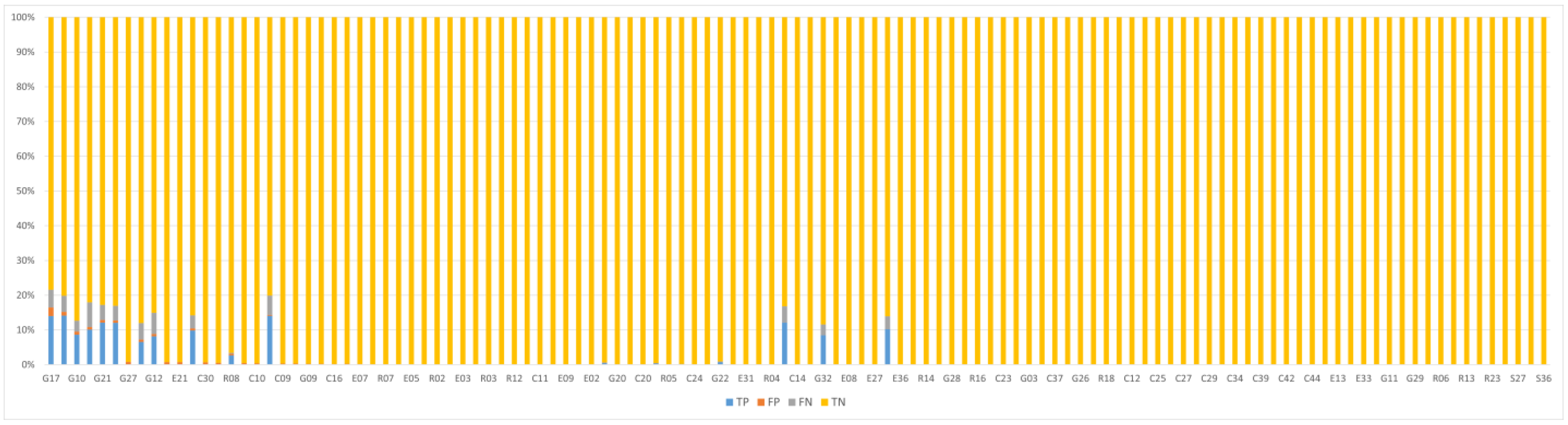
• True Positive (TP): The number of data points correctly identified as anomalies, i.e., points that truly belong to the attack interval and are correctly detected by the model.
• True Negative (TN): The number of data points correctly identified as normal, i.e., points that are outside the attack interval and are not falsely marked as anomalous.
• False Positive (FP): The number of data points incorrectly identified as anomalies, i.e., normal points that were mistakenly flagged as anomalous.
• False Negative (FN): The number of data points incorrectly identified as normal, i.e., points within the attack interval that the model failed to detect as anomalies.

Based on these categories, the following performance metrics of the model are computed to evaluate its effectiveness in identifying spoofing anomalies.

• Precision: The proportion of predicted anomalies that are actually true anomalies:

  $$\mathrm{Precision}={\displaystyle \frac{TP}{TP+FP}}$$

  (4)
• Recall (or True Positive Rate): Measures the model’s ability to correctly detect actual anomalies. It represents the proportion of true anomalies that were successfully identified:

  $$\mathrm{Recall}={\displaystyle \frac{TP}{TP+FN}}$$

  (5)
• F1-score: Represents the harmonic mean between precision and recall. It balances the trade-off between false positives and false negatives:

  $$\mathrm{F}1-\mathrm{score}={\displaystyle \frac{2\ast Precision\ast Recall}{Precision+Recall}}$$

  (6)

Next, the results in

Table 4. Overall performance metrics based on different scaling coefficients.

Scaling Coefficient	Precision (%)	Recall (%)	F1-Score (%)
k = 2.0	82.3	95.1	89.3
k = 2.5	88.6	91.4	90.0
k = 3.0	91.8	89.7	90.7
k = 3.5	94.1	81.5	87.3
k = 4.0	94.5	73.2	83.1

demonstrate that the choice of threshold scaling coefficient k has a significant impact on detection performance. As k increases, the model becomes more conservative, leading to higher precision but lower recall.

In particular, when k = 2.0, the model achieves a high recall of 95.1%, ensuring that most spoofing anomalies are detected, but at the cost of more false positives (precision = 82.3%). Conversely, when k = 4.0, the precision peaks at 94.5%, but the recall drops significantly to 73.2%, indicating that many true anomalies are missed. The best balance between sensitivity and reliability is achieved at k = 3.0, where the model attains a precision of 91.8%, a recall of 89.7%, and a maximum F1-score of 90.7%.

Figure 24 shows the normalized confusion matrix components (TP, FP, FN, TN) for each satellite. As expected, the vast majority of samples are true negatives (TN), reflecting the structure of the test data. True positives (TP) and false positives (FP) are concentrated in a limited number of satellites, which is consistent with the known spoofing interval. Importantly, false negatives (FN) are rare, indicating strong detection sensitivity. Overall, the model exhibits precise and stable behavior across the satellite network, with very low false alarm rates and consistent performance on the affected signals.

Next, in Figure 25, the False Positive Rate (FPR) is presented for each satellite. FPR quantifies the proportion of normal (non-spoofed) data points that were incorrectly flagged as anomalies. This metric is essential for evaluating the model’s reliability, especially in scenarios where false alarms can affect system trust. As shown, the vast majority of satellites exhibit an FPR close to zero, confirming the model’s conservative and robust behavior. A small number of satellites (e.g., G17, G10) display slightly elevated FPR values, which may be attributed to local signal variability or modeling sensitivity.

5.2.4. LSTM Attack Detection

Based on the LSTM test architecture and test data presented above, the figures below show the results of the proposed mechanism. Thus, the first parameter tested is the Pseudorange observation codes for the presented GNSS and their frequency bands. Figure 26 shows the results of algorithm testing for this parameter, where the values considered as anomalies were marked with red x symbols. From the figure, we can see that the algorithm has marked the attack period very well, especially for the L1 band of the GPS. However, we can observe some outlier points that were marked as anomalies. This is due to the fact that the value structure those points were part of was not large enough for the algorithm to determine their validity. Therefore, we can consider those points as false alarms. We can also note that when the attack was launched, the algorithm flagged this for Galileo, GLONASS, Beidou, SBAS, and QZSS. This is because the parameter suddenly suffered an unexpected drop and the structure formed by the parameter is not complete as expected.

In the following figure, Figure 27, the results of the algorithm test for Carrier Phase observation codes are presented.

Similarly, anomaly values are marked with red x symbols on the graphs. Similarly to the Pseudorange parameter, in the case of the Carrier Phase parameter, the algorithm marked the abnormal values of the Carrier Phase during the period when the attack occurred. We also observe that the number of abnormal points associated with false alarms has increased. Similarly, this is due to incomplete sequences of the parameter. These incomplete sequences can be associated with temporary loss of signal received from satellites, disturbing effects or residual signals. The next parameter tested using the algorithm is Doppler Shift and Figure 28 presents the testing results.

The figure shows the test data for the observation codes of this parameter, with the points identified as anomalies marked with red x symbols. From the graph, it can be seen that the parameter values for the GPS L1 band during the attack period were flagged as anomalies. Also, for the other systems and frequency bands, the beginning of the attack was marked and identified. Similarly, isolated values that do not show a complete sequence are flagged as outliers. For SBAS and QZSS, we can observe some outlier points that do not follow the parameter pattern and were flagged by the algorithm. The last parameter tested is Signal Strength and Figure 29 shows the results of the algorithm testing.

According to the graphs, we observe the same behavior of the algorithm during the period of the attack as well as for the isolated values that did not develop a complete pattern. Also, for the other systems that had no parameter data at the time of the attack, the beginning of the attack was flagged as an anomaly.

Given these results, we can conclude that the algorithm is efficient in detecting this type of attack. However, further optimizations may be required to improve its sensitivity and robustness in detecting more subtle anomalies, to reduce false positives, or to handle edge cases where the spoofed signals closely mimic legitimate ones. This can be improved by integrating additional detection mechanisms. For example, by analyzing the .nav file, satellite ephemerides and clock correction data can be extracted to reconstruct expected satellite positions and signal parameters. Comparing these expected values with the actual observations can help identify inconsistencies caused by spoofed signals, thereby enhancing the accuracy and reliability of the detection process.

6. Conclusions

This study presented a detection approach for GNSS spoofing attacks based on LSTM reconstruction models applied to raw observation codes (Pseudorange, Carrier Phase, Doppler, and Signal Strength) extracted from RINEX data. The proposed pipeline covered both data acquisition in a clean environment and simulation of spoofing scenarios using SDR-based emissions, enabling the analysis of signal distortions under controlled attack conditions.

Compared to other spoofing detection methods described in the literature including consistency checks (e.g., RAIM variants), cryptographic authentication, and supervised learning models such as SVM and CNN, the current method operates at the final observation layer of the GNSS signal chain and requires no hardware modifications or external reference receivers. In contrast to approaches such as [43], which transform time series into images and apply image anomaly detection with knowledge distillation, our approach maintains the native temporal structure of the GNSS signal and emphasizes time-aligned, multi-code dependencies for detection.

The experimental evaluation included analysis across multiple GNSS constellations and satellites, showing that the proposed model is able to identify spoofing-induced anomalies reflected in abrupt variations in the observation codes. Classification metrics, as presented in Table 4, varied with the threshold sensitivity (k), with F1-scores above 90% in several configurations. Detection performance remained stable across satellites affected by the spoofing emission, while false positives were limited to isolated cases, typically linked to signal dropout or discontinuities in observation sequences. Also, the use of cross-code validation where an anomaly is confirmed only when all four observation codes indicate abnormal behavior at the same timestamp significantly improved the detection precision and reduced isolated false alarms. In addition, False Positive Rates (FPRs) remained below 2% for the majority of the satellites, as illustrated in Figure 25. These values reflect the method’s ability to generalize across multiple signals, while controlling false alarms even in noisy or partially degraded GNSS data.

Although the present study focused on a single spoofing scenario, the results suggest that the method is applicable to detection tasks in scenarios where more complex spoofing forms may occur. Future work will aim to expand comparative experiments with other ML-based methods (e.g., CNN-LSTM hybrids, Transformer-based models), as well as to test model behavior under dynamic motion and across different hardware receivers. Furthermore, fusion with navigation data (e.g., RINEX NAV files) and cross-verification strategies are being considered to strengthen anomaly confirmation.

References

1. Yasyukevich, Y.V.; Zhang, B.; Devanaboyina, V.R. Advances in GNSS Positioning and GNSS Remote Sensing. Sensors 2024, 24, 1200. [Google Scholar] [CrossRef]
2. Teunissen, P.J.G.; Montenbruck, O. Springer Handbook of Global Navigation Satellite Systems; Springer: Cham, Switzerland, 2017. [Google Scholar]
3. Gao, J. A Brief Discussion on Understanding GNSS and Navigation Engineering. Acad. J. Sci. Technol. 2024, 11, 248–249. [Google Scholar]
4. Zalewski, P.; Bąk, A.; Bergmann, M. Evolution of Maritime GNSS and RNSS Performance Standards. Remote Sens. 2022, 14, 5291. [Google Scholar] [CrossRef]
5. John, W.B. The Navstar Global Positioning System. In Position, Navigation, and Timing Technologies in the 21st Century: Integrated Satellite Navigation, Sensor Systems, and Civil Applications; IEEE: New York, NY, USA, 2021; pp. 65–85. [Google Scholar]
6. Pinninti, K.; Veligatla, S.B.; Gireddy, A.K.R. Extraction of Satellite Data and Generation of C/A Codes for GPS Signals on FPGA. In Proceedings of the 2024 International Conference on Integrated Circuits and Communication Systems (ICICACS), Raichur, India, 23–24 February 2024; pp. 1–4. [Google Scholar]
7. Xia, F.; Wang, C.; Chen, D.; Wu, J.; Ye, S.; Sun, W. Estimation of antenna phase center offsets for BeiDou IGSO and MEO satellites. GPS Solut. 2020, 24, 90. [Google Scholar]
8. Lu, J.; Guo, X.; Su, C. Global capabilities of BeiDou Navigation Satellite System. Satell. Navig. 2020, 1, 27. [Google Scholar] [CrossRef]
9. Andrei, C.-O.; Johansson, J.; Koivula, H.; Poutanen, M. Signal performance analysis of the latest quartet of Galileo satellites during the first operational year. In Proceedings of the 2020 International Conference on Localization and GNSS (ICL-GNSS), Tampere, Finland, 2–4 June 2020; pp. 1–6. [Google Scholar]
10. Jiao, F.; Yu, X.; Hu, Y. Performance of GNSS space service for geostationary autonomous operations. J. Navig. 2024, 77, 257–275. [Google Scholar] [CrossRef]
11. Pan, L.; Pei, G.; Yu, W.; Zhang, Z. Assessment of IRNSS-Only Data Processing: Availability, Single-Frequency SPP and Short-Baseline RTK. Remote Sens. 2022, 14, 2462. [Google Scholar]
12. Karasawa, K.; Takizawa, Y.; Sasaki, Y.; Hirota, Y.; Ashida, K.; Karakama, T.; Kaneko, T. Satellite Positioning System with Active Antenna for QZSS. In Proceedings of the 2021 IEEE 10th Global Conference on Consumer Electronics (GCCE), Kyoto, Japan, 12–15 October 2021; pp. 65–68. [Google Scholar]
13. Gu, H.; Rao, Y.; Zou, D.; Shi, H.; Guo, Y. Analysis of Multipath Characteristics of Quasi-Zenith Satellite System L5 Frequency Point. Remote Sens. 2025, 17, 889. [Google Scholar]
14. Lim, C.; Park, B.; Yun, Y. L1 SFMC SBAS Message for Service Expansion of Multi-Constellation GNSS Support. IEEE Access 2023, 11, 81690–81710. [Google Scholar] [CrossRef]
15. GPS Space Segment. Available online: https://www.gps.gov/systems/gps/space/ (accessed on 19 February 2025).
16. Galileo Space Segment. Available online: https://www.gsc-europa.eu/galileo/system/ (accessed on 19 February 2025).
17. GLONASS Space Segment. Available online: https://glonass-iac.ru/en/about_glonass/ (accessed on 19 February 2025).
18. Beidou Space Segment. Available online: https://gssc.esa.int/navipedia/index.php/BeiDou_Space_Segment (accessed on 19 February 2025).
19. Maciejewska, A.; Maciuk, K. Research using GNSS (Global Navigation Satellite System) products—A comprehensive literature review. J. Appl. Geod. 2025. [Google Scholar] [CrossRef]
20. Meng, L.; Yang, L.; Yang, W.; Zhang, L. A Survey of GNSS Spoofing and Anti-Spoofing Technology. Remote Sens. 2022, 14, 4826. [Google Scholar] [CrossRef]
21. Zhong, M.; Li, H.; Lu, M. Analysis and Validation of Distributed GNSS Spoofing Threat. Eng. Proc. 2025, 88, 42. [Google Scholar]
22. Dasgupta, S.; Ahmed, A.; Rahman, M.; Bandi, T.N. Unveiling the Stealthy Threat: Analyzing Slow Drift GPS Spoofing Attacks for Autonomous Vehicles in Urban Environments and Enabling the Resilience. arXiv 2024, arXiv:2401.01394. [Google Scholar]
23. Ma, X.; Han, C.; Jin, R.; Wang, D.; Bai, P.; Zhen, W. Study on GNSS Spoofing Interference Detection Method in Urban Multipath Environment Based on CNN and Clustering Model. In Proceedings of the 2023 Cross Strait Radio Science and Wireless Technology Conference (CSRSWTC), Guilin, China, 10–13 November 2023; Available online: https://ieeexplore.ieee.org/document/10427220 (accessed on 12 February 2025).
24. Motallebighomi, M.; Sathaye, H.; Singh, M.; Ranganathan, A. Cryptography is not enough: Relay attacks on authenticated GNSS signals. arXiv 2022, arXiv:2204.11641. [Google Scholar]
25. The Hindu Businessline. Report: “GPS Jamming Near Conflict Zones Affect Cargo Ships Transiting Mediterranean and the Black Sea” by Teraja Simhan. Available online: https://www.thehindubusinessline.com/news/world/gps-jamming-near-conflict-zones-affect-cargo-ships-transiting-mediterranean-and-the-black-sea/article68038995.ece (accessed on 12 February 2025).
26. AIN. Report: “GPS Spoofing Incidents Increase in Middle East” by Kerry Lynch. Available online: https://www.ainonline.com/aviation-news/air-transport/2023-11-08/gps-spoofing-incidents-increase-middle-east (accessed on 12 February 2025).
27. The Wall Street Journal. Report: “Electronic Warfare Spooks Airlines, Pilots and Air-Safety Officials”. Available online: https://ops.group/dashboard/wp-content/uploads/2024/09/GPS-Spoofing-Final-Report-OPSGROUP-WG-OG24.pdf (accessed on 12 February 2025).
28. GPS WORLD. Report: “GNSS Spoofing Threatens Airline Safety, Alarming Pilots and Aviation Officials” by Jesse Khalil. Available online: https://www.gpsworld.com/gnss-spoofing-threatens-airline-safety-alarming-pilots-and-aviation-officials/ (accessed on 12 February 2025).
29. Gao, Y.; Li, G. A Slowly Varying Spoofing Algorithm Avoiding Tightly-Coupled GNSS/IMU With Multiple Anti-Spoofing Techniques. IEEE Trans. Veh. Technol. 2022, 71, 8864–8876. [Google Scholar] [CrossRef]
30. Kawamoto, S.; Takamatsu, N.; Abe, S. RINGO: A RINEX pre-processing software for multi-GNSS data. Earth Planets Space 2023, 75, 54. [Google Scholar] [CrossRef]
31. Han, J.; Lee, S.J.; Yun, H.S.; Kim, K.B.; Bae, S. WPyRINEX: A new multi-purpose Python package for GNSS RINEX data. Peer J. Comput. Sci. 2024, 10, e1800. [Google Scholar]
32. Medina, E.T.; Lohan, E.S. GNSS Spoofing Modeling and Consistency-Check-Based Spoofing Mitigation with Android Raw Data. Electronics 2025, 14, 898. [Google Scholar]
33. Kabir, M.H.; Hasan, M.A.; Shin, W. A Precise Positioning Method with Integration of GNSS and Doppler Shift Based Positioning using LEO Satellite. In Proceedings of the 2023 14th International Conference on Information and Communication Technology Convergence (ICTC), Jeju Island, Republic of Korea, 11–14 October 2023; pp. 315–317. [Google Scholar]
34. Ghizzo, E.; Pena, A.G.; Lesouple, J.; Milner, C.; Macabiau, C. Assessing GNSS Carrier-to-Noise-Density Ratio Estimation in The Presence of Meaconer Interference. In Proceedings of the ICASSP 2024—2024 IEEE International Conference on Acoustics, Speech and Signal Processing (ICASSP), Seoul, Republic of Korea, 14–19 April 2024; pp. 8971–8975. [Google Scholar]
35. Weikong, Q.; Zhang, Y.; Liu, X. A GNSS anti-spoofing technology based on Doppler shift in vehicle networking. In Proceedings of the 2016 International Wireless Communications and Mobile Computing Conference, Paphos, Cyprus, 5–9 September 2016; IEEE: New York, NY, USA, 2016; pp. 725–729. [Google Scholar]
36. Yang, B.; Tian, M.; Ji, Y.; Cheng, J.; Xie, Z.; Shao, S. Research on GNSS Spoofing Mitigation Technology Based on Spoofing Correlation Peak Cancellation. IEEE Commun. Lett. 2022, 26, 3024–3028. [Google Scholar] [CrossRef]
37. Jin, R.; Yan, J.; Cui, X.; Yang, H.; Zhen, W.; Gu, M.; Ji, G. A Spoofing Detection and Direction-Finding Approach for Global Navigation Satellite System Signals Using Off-the-Shelf Anti-Jamming Antennas. Remote Sens. 2025, 17, 864. [Google Scholar] [CrossRef]
38. Galan, A.; O’Driscoll, C.; Fernandez-Hernandez, I.; Pollin, S. Sensitivity Analysis of Galileo OSNMA Cross-Authentication Sequences. Eng. Proc. 2025, 88, 12. [Google Scholar]
39. Hammarberg, T.; García, J.M.V.; Alanko, J.N.; Bhuiyan, M.Z.H. An Experimental Performance Assessment of Galileo OSNMA. Sensors 2024, 24, 404. [Google Scholar] [CrossRef]
40. Semanjski, S.; Semanjski, I.; De Wilde, W.; Muls, A. Use of Supervised Machine Learning for GNSS Signal Spoofing Detection with Validation on Real-World Meaconing and Spoofing Data—Part I. Sensors 2020, 20, 1171. [Google Scholar] [CrossRef] [PubMed]
41. Pervysheva, Y.; Käppi, J.; Syrjärinne, J.; Nurmi, J.; Lohan, E.S. Multi-Receiver Ensemble Machine-Learning Techniques for GNSS Spoofing Detection with Generalisability Approach. In Proceedings of the 2024 32nd Telecommunications Forum (TELFOR), Belgrade, Serbia, 26–27 November 2024; pp. 1–4. [Google Scholar]
42. Iqbal, A.; Aman, M.N.; Sikdar, B. A Deep Learning Based Induced GNSS Spoof Detection Framework. IEEE Trans. Mach. Learn. Commun. Netw. 2024, 2, 457–478. [Google Scholar]
43. Park, H.; Jang, H. Enhancing Time Series Anomaly Detection: A Knowledge Distillation Approach with Image Transformation. Sensors 2024, 24, 8169. [Google Scholar] [CrossRef]
44. Lee, G.; Yoon, Y.; Lee, K. Anomaly Detection Using an Ensemble of Multi-Point LSTMs. Entropy 2023, 25, 1480. [Google Scholar] [CrossRef]
45. Lin, Y.; Xie, Z.; Chen, T.; Cheng, X.; Wen, H. Image privacy protection scheme based on high-quality reconstruction DCT compression and nonlinear dynamics. Expert Syst. Appl. 2024, 257, 124891. [Google Scholar] [CrossRef]
46. Wang, F.; Jiang, Y.; Zhang, R.; Wei, A.; Xie, J.; Pang, X. A Survey of Deep Anomaly Detection in Multivariate Time Series: Taxonomy, Applications, and Directions. Sensors 2025, 25, 190. [Google Scholar] [CrossRef]
47. Xu, J.; Li, K.; Li, D. An Automated Few-Shot Learning for Time-Series Forecasting in Smart Grid Under Data Scarcity. IEEE Trans. Artif. Intell. 2024, 5, 2482–2492. [Google Scholar] [CrossRef]
48. Xu, J.; Li, K.; Li, D. Multioutput Framework for Time-Series Forecasting in Smart Grid Meets Data Scarcity. IEEE Trans. Ind. Inform. 2024, 20, 11202–11212. [Google Scholar]
49. Tropea, M.; Arieta, A.; De Rango, F.; Pupo, F. A Proposal of a Troposphere Model in a GNSS Simulator for VANET Applications. Sensors 2021, 21, 2491. [Google Scholar] [CrossRef] [PubMed]
50. Carlin, L.; Hauschild, A.; Montenbruck, O. Precise point positioning with GPS and Galileo broadcast ephemerides. GPS Solut. 2021, 25, 77. [Google Scholar]
51. Maltsev, A.S.; Burtsev, S.Y.; Pecheritsa, D.S. Evaluation of Root Mean Square of Global Navigation Satellite Systems Receiver Carrier Phase Measurement Error. In Proceedings of the 2024 IEEE 3rd International Conference on Problems of Informatics, Electronics and Radio Engineering (PIERE), Novosibirsk, Russia, 15–17 November 2024; pp. 50–55. [Google Scholar]
52. Sun, M.-T.; Feng, W.-C.; Lai, T.-H.; Yamada, K.; Okada, H.; Fujimura, K. GPS-based message broadcast for adaptive inter-vehicle communications, Vehicular Technology Conference Fall 2000. In Proceedings of the IEEE VTS Fall VTC2000. 52nd Vehicular Technology Conference (Cat. No.00CH37152), Boston, MA, USA, 24–28 September 2000; Volume 6, pp. 2685–2692. [Google Scholar]
53. Liu, S.; Li, S.; Zheng, J.; Fu, Q.; Yuan, Y. C/N0 Estimator Based on the Adaptive Strong Tracking Kalman Filter for GNSS Vector Receivers. Sensors 2020, 20, 739. [Google Scholar] [CrossRef] [PubMed]
Figure 1. Overview of GNSS, RNSS, and SBAS satellite constellations.
Information 16 00502 g001
Figure 2. GNSS and RNSS frequency bands and signals.
Information 16 00502 g002
Figure 3. Training topology and systems under test.
Information 16 00502 g003
Figure 4. Ser2net command (red box) for TCP/UDP connection setup to GNSS teletype port.
Information 16 00502 g004
Figure 5. U-center application, active remote connection to GNSS Box.
Information 16 00502 g005
Figure 6. RTKLib interface for UBX file conversion to RINEX standard.
Information 16 00502 g006
Figure 7. Observation file header and epoch format from RINEX standard.
Information 16 00502 g007
Figure 8. RINEX training data processing workflow.
Information 16 00502 g008
Figure 9. Testing topology and systems under test.
Information 16 00502 g009
Figure 10. Installing a TCXO on the HackRF One board.
Information 16 00502 g010
Figure 11. Python application for signal generation and transmission.
Information 16 00502 g011
Figure 12. MJD parameters and number of satellites from training data.
Information 16 00502 g012
Figure 13. Pseudorange observation codes from training data for GPS, Galileo, GLONASS, Beidou, and QZSS.
Information 16 00502 g013
Figure 14. Carrier Phase observation codes from training data for GPS, Galileo, GLONASS, Beidou, and QZSS.
Information 16 00502 g014
Figure 15. Doppler Shift observation codes from training data for GPS, Galileo, GLONASS, Beidou, and QZSS.
Information 16 00502 g015
Figure 16. Signal Strength observation codes from training data for GPS, Galileo, GLONASS, Beidou, and QZSS.
Information 16 00502 g016
Figure 17. LSTM training computational resources; (a) total train time per constellation; (b) total memory footprint.
Information 16 00502 g017
Figure 18. Training loss and validation loss for satellite signals of each constellation.
Information 16 00502 g018
Figure 19. MJD parameters and number of satellites from testing data.
Information 16 00502 g019
Figure 20. Pseudorange observation codes from testing data for GPS, Galileo, GLONASS, Beidou, and QZSS with attack period marked with red dashed line.
Information 16 00502 g020
Figure 21. Carrier Phase observation codes from testing data for GPS, Galileo, GLONASS, Beidou, and QZSS with attack period marked with red dashed line.
Information 16 00502 g021
Figure 22. Doppler Shift observation codes from testing data for GPS, Galileo, GLONASS, Beidou, and QZSS with attack period marked with red dashed line.
Information 16 00502 g022
Figure 23. Signal Strength observation codes from testing data for GPS, Galileo, GLONASS, Beidou, and QZSS with attack period marked with red dashed line.
Information 16 00502 g023
Figure 24. Proportional distribution of classification outcomes (TP, FP, FN, TN) for each GNSS satellite.
Information 16 00502 g024
Figure 25. False Positive Rate per satellite.
Information 16 00502 g025
Figure 26. LSTM attack detection for Pseudorange observation codes from testing data with attack period marked with red dashed line.
Information 16 00502 g026
Figure 27. LSTM attack detection for Carrier Phase observation codes from testing data with attack period marked with red dashed line.
Information 16 00502 g027
Figure 28. LSTM attack detection for Doppler observation codes from testing data with attack period marked with red dashed line.
Information 16 00502 g028
Figure 29. LSTM attack detection for Signal Strength observation codes from testing data with attack period marked with red dashed line.
Information 16 00502 g029