Automated Crack Width Measurement in 3D Models: A Photogrammetric Approach with Image Selection

Abstract

Structural cracks can critically undermine infrastructure integrity, driving the need for precise, scalable inspection methods beyond conventional visual or 2D image-based approaches. This study presents an automated system integrating photogrammetric 3D reconstruction with deep learning to quantify crack dimensions in a spatial context. Multiple images are processed via Agisoft Metashape to generate high-fidelity 3D meshes. Then, a subset of images are automatically selected based on camera orientation and distance, and a deep learning algorithm is applied to detect cracks in 2D images. The detected crack edges are projected onto a 3D mesh, enabling width measurements grounded in the structure’s true geometry rather than perspective-distorted 2D approximations. This methodology addresses the key limitations of traditional methods (parallax, occlusion, and surface curvature errors) and shows how these limitations can be mitigated by spatially anchoring measurements to the 3D model. Laboratory validation confirms the system’s robustness, with controlled tests highlighting the importance of near-orthogonal camera angles and ground sample distance (GSD) thresholds to ensure crack detectability. By synthesizing photogrammetry and a convolutional neural network (CNN), the framework eliminates subjectivity in inspections, enhances safety by reducing manual intervention, and provides engineers with dimensionally accurate data for maintenance decisions.

1. Introduction

Cracks in structural systems, such as bridges and pavements, pose significant risks to safety and longevity. They compromise load-bearing capacity, accelerate deterioration through water ingress and corrosion, and account for approximately 76% of bridge collapses globally [1]. Crack width measurement is critical for assessing structural health, guiding maintenance decisions, and ensuring public safety [2]. Despite this urgency, conventional inspection methods, such as human visual observation and telescopic surveys, remain inefficient, subjective, and impractical for large-scale infrastructure like high-pier bridges [3]. These approaches struggle with accessibility (e.g., bridge bottoms and tower tops), expose inspectors to safety hazards, and lack the precision required for rapid, quantitative assessments. Such limitations underscore the need for advanced, automated solutions to replace outdated practices.

While imaging technologies have emerged as tools for defect detection, relying solely on 2D images introduces challenges. These image-based inspections often fail to capture spatial context, scale, or three-dimensional geometry, limiting their ability to quantify crack dimensions accurately. Furthermore, manual crack detection, whether via images or on-site surveys, is labor-intensive, time-consuming, and dependent on operator expertise [4,5]. These shortcomings highlight the necessity of integrating imaging with advanced computational frameworks to derive actionable, dimensionally accurate insights.

In this context, the study presented in [6] marks a significant advancement by addressing these limitations through a UAV-based crack assessment system combined with 3D reconstruction techniques. The proposed methodology overcomes challenges of perspective and geometric distortions while enhancing the accuracy and efficiency of crack detection in large-scale structures, but lacks algorithmic transparency. Similarly, Ref. [7] proposes a UAV-based system for automated bridge inspections, integrating real-time crack detection with the possibility of 3D bridge modeling and crack localisation. It advances real-time detection with integrated 3D modeling, yet its proprietary drone system limits scalability. Contrasting common photogrammetric methods, Ref. [8] introduces a stereoscopic imaging system for UAV-based 3D crack assessment. By employing stereo images, this approach captures inherent depth data, reducing reliance on multi-angle image sequences. The framework combines adaptive crack detection algorithms with stereo disparity mapping to spatially reconstruct cracks using projective ray intersections. However, its applicability is restricted to localized regions. Meanwhile, Ref. [9] proposes a UAV methodology for large-scene bridge inspections, prioritizing the efficient detection of cracks exceeding specified width thresholds through optimized aerial image acquisition. This approach employs strategic flight paths and vertical photography distances to balance crack detectability with broad structural coverage, leveraging innovations such as background denoising via grid segmentation. But it fails to detect cracks in occluded areas like bridge undersides due to reliance on vertical imaging.

While these studies are related to advances in crack inspection systems, parallel research focuses on refining the algorithmic foundations of crack detection itself, addressing challenges in segmentation accuracy, computational efficiency, and morphological adaptability. Recent innovations demonstrate progress in deep learning-based approaches. For instance, Ref. [10] highlights the efficacy of transfer learning with pre-trained fully convolutional networks, showing that model initialization using large-scale datasets enhances classification accuracy while reducing training data dependency, which is a critical advantage for engineering applications. Expanding on this, Ref. [11] pioneers the adaptation of U-Net, where it is developed first on a biomedical segmentation architecture [12], to crack detection. By integrating encoder–decoder structures with skip connections, the model achieves robust performance with limited training data, demonstrating generalizability across diverse structural contexts. Subsequent work by [13] introduces U-Net refinements such as mirror padding, multi-scale feature fusion, and residual linear attention modules to optimize feature alignment and pooling efficiency.

Building on these algorithmic advancements, recent research extends these networks to multi-task frameworks for concurrent crack characterization. For example, Ref. [14] introduces a dual-task model combining crack segmentation and centerline prediction, circumventing traditional post-processing steps like error-prone skeletonization. Through parallel decoders, one for segmentation and another for centerline extraction, the approach directly predicts crack morphology features, minimizing artifacts from manual post-processing.

As global infrastructure systems face aging and environmental stressors, such innovations are vital to safeguarding structural integrity and extending service life [15,16,17].

Convolutional neural networks (CNNs) have emerged as powerful tools for automated crack segmentation and analysis; however, a critical gap persists in integrating these algorithms with photogrammetric systems without dependence on specialized hardware or custom software, limiting their adaptability and scalability. To bridge this gap, this study introduces a practical workflow that synergizes commercially available photogrammetry tools, specifically Agisoft Metashape Professional Version 2.1.0, a commercially established and accessible photogrammetry tool, with CNN segmentation models. By developing a custom script to automate 3D crack detection and leveraging Metashape’s established capabilities, the proposed system eliminates the need for custom hardware or software redesign. This approach prioritizes flexibility and accessibility, accommodating diverse image acquisition techniques while ensuring compatibility with widely accessible computational resources—key advantages for real-world structural assessments.

Building on this foundation, this study introduces an automated photogrammetry-based framework that seamlessly integrates multi-image analysis with 3D modeling and CNN-driven crack detection. By reconstructing high-fidelity 3D meshes from images optimized for camera orientation and distance, the system minimizes perspective distortion while preserving geometric accuracy. The CNN architecture, at its core, generalizes across diverse crack morphologies and lighting conditions, outperforming traditional methods [18] and eliminating manual intervention. Detected cracks are then spatially contextualized by projecting them onto the 3D model, enabling precise width measurements that transcend the planar limitations of 2D imaging.

Conventional crack detection methods, relying on 2D images, are inherently constrained by distortions caused by parallax, occlusions, and surface curvature. For example, cracks on curved surfaces may appear to vary in width across images due to differences in camera orientation, undermining measurement reliability. To resolve these limitations, this study introduces a novel approach where crack edges identified in 2D images are projected onto a 3D mesh reconstructed via photogrammetry using Agisoft Metashape. This ensures measurements are based on the structure’s physical geometry, eliminating perspective distortions inherent to individual images.

Images are systematically selected based on their orientation relative to the crack surface, including the angle between the camera’s optical axis and the local surface, as well as the distance from the camera to the target. This selective strategy prioritizes images with near-orthogonal viewing angles and optimal working distances, enhancing crack visibility and segmentation accuracy.

2. Preliminary Procedures

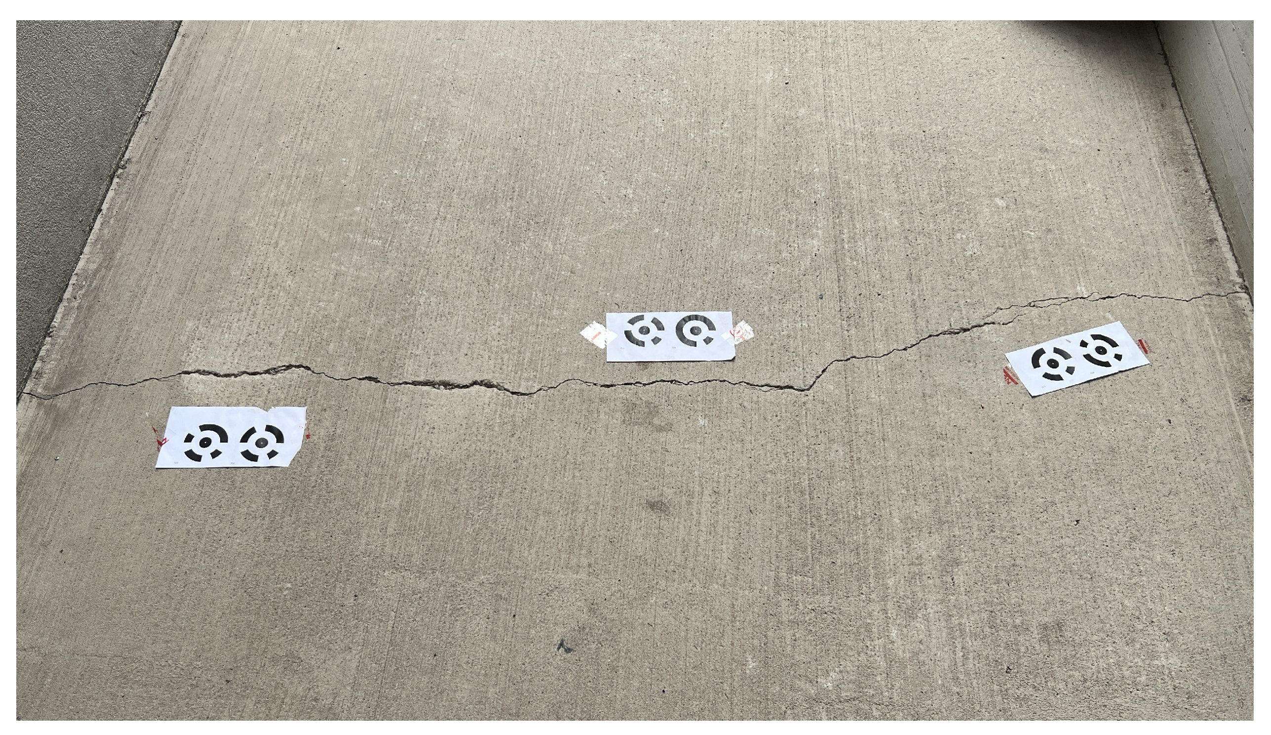
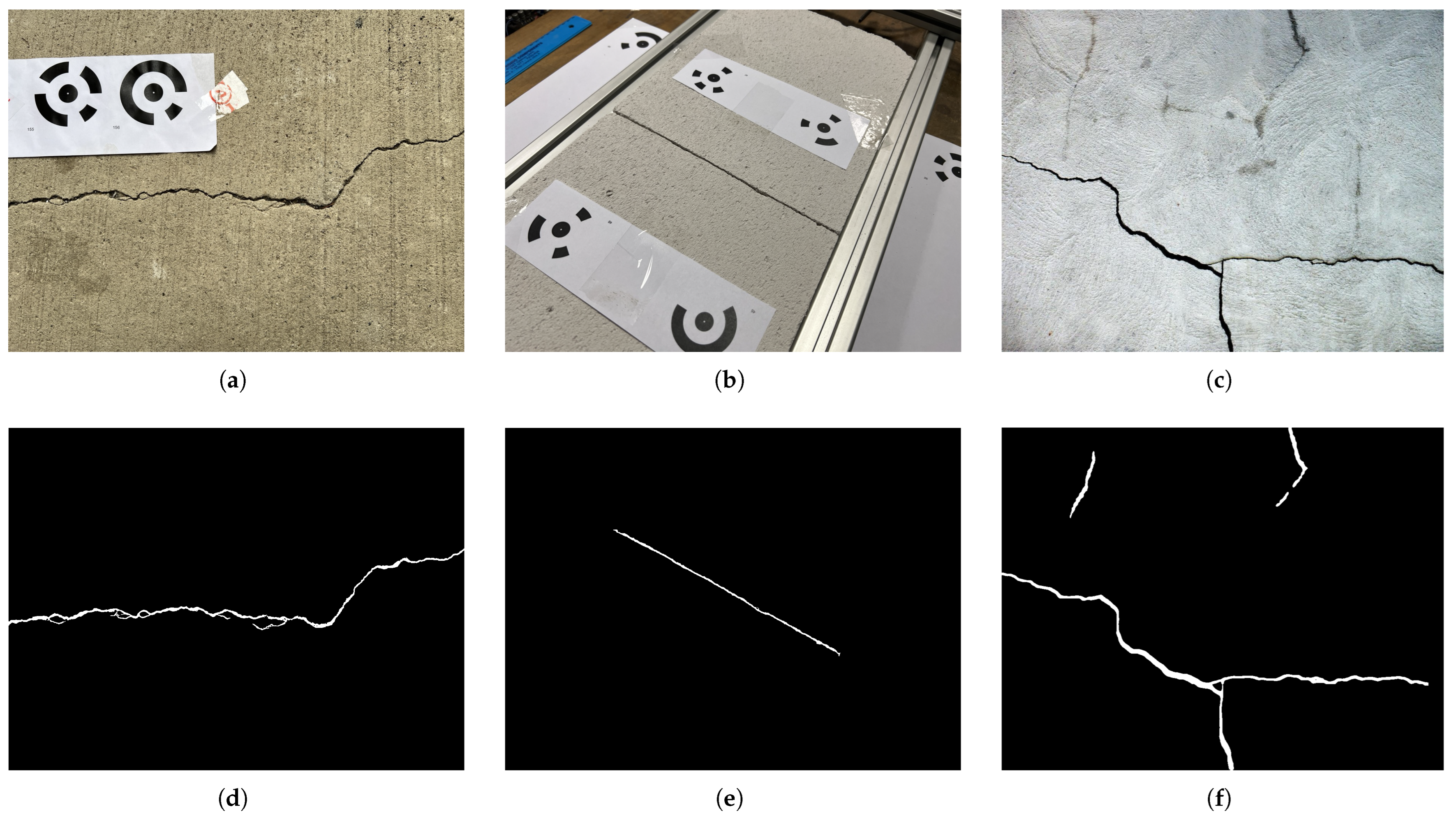
2.1. Image Acquisition on Site

A structured image acquisition process was implemented to ensure accurate 3D reconstruction and crack assessment. A high-resolution digital camera (5 MP or higher) was used, avoiding ultra-wide-angle and fisheye lenses to minimize distortions. Key camera parameters—including ISO level, exposure time, and aperture size—were optimized to balance image quality and clarity, in accordance with the guidelines for photogrammetric processing provided in the Agisoft Metashape User Manual [19]. Circular targets were placed around or on the object, with the measured distances between them providing a reference for scene scaling. Although targets are preferred for their accuracy, in cases where using them is not possible, distinct features on the object itself, such as corners, edges, or other identifiable elements, can be manually selected and their known distances recorded. The related scene can be scaled using these manually selected distances.

High overlap between images ensured successful alignment in Metashape, while additional close-up images captured fine details for crack assessment. The process adhered to best practices to produce high-fidelity 3D models suitable for both reconstruction and crack analysis. An example scene created with target can be seen in Figure 1.

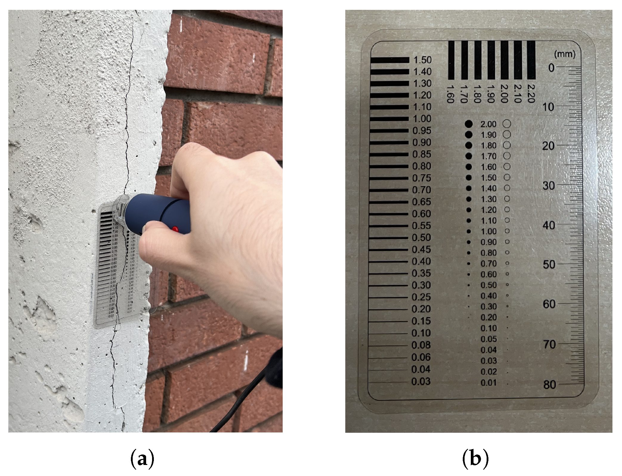
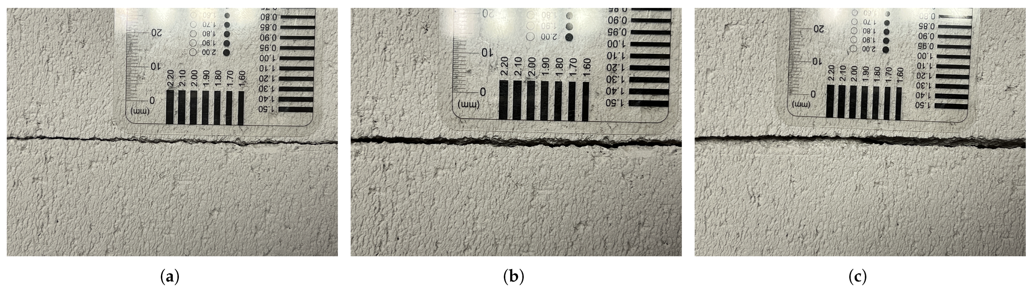
2.2. Manual Crack Measurements on Site

To validate the results of the automated crack detection system, manual measurements were conducted on site using a microscope camera and a crack gauge. The microscope camera allowed for a detailed examination of cracks, capturing high-resolution images that revealed intricate details often missed by conventional methods. A crack gauge, as seen in Figure 2b, was positioned within the field of view to provide a known reference distance for measurement calibration. The combination of these tools can be seen in Figure 2a.

A custom measurement tool was developed to load these images and enable the manual definition of crack widths in pixel units. The user interface of this tool can be seen in Figure 3. The tool compared the pixel dimensions of the cracks to the known distance on the crack gauge, ensuring accurate measurements. Multiple measurements were taken at different locations along each crack to obtain the distribution of crack widths, and statistical methods were applied to these results to facilitate a comparison with the automated measurements from the proposed method. These statistical methods are explained in detail in Section 4.

While cracks may appear as simple gaps between two surfaces when viewed from a distance, the microscope camera revealed more complex details, such as spalled regions resulting from material loss. In this study, the focus was specifically on the crack regions, excluding spalled areas, to ensure accurate and consistent measurements. This manual validation process provided a reliable benchmark for evaluating the performance of the automated crack detection system.

2.3. 3D Scene Reconstruction in Metashape

The 3D reconstruction in Agisoft Metashape started with feature detection and matching across overlapping images. The camera positions were estimated, and tie points were manually cleaned to focus on the object. An initial mesh was created for image masking, refining it to remove background elements. Depth maps were generated, producing a dense point cloud that was manually refined for accuracy.

The final 3D mesh, derived from the refined point cloud, provided a high-quality surface representation. Texturing was optional for visualization. An example of the final textured mesh can be seen in Figure 4.

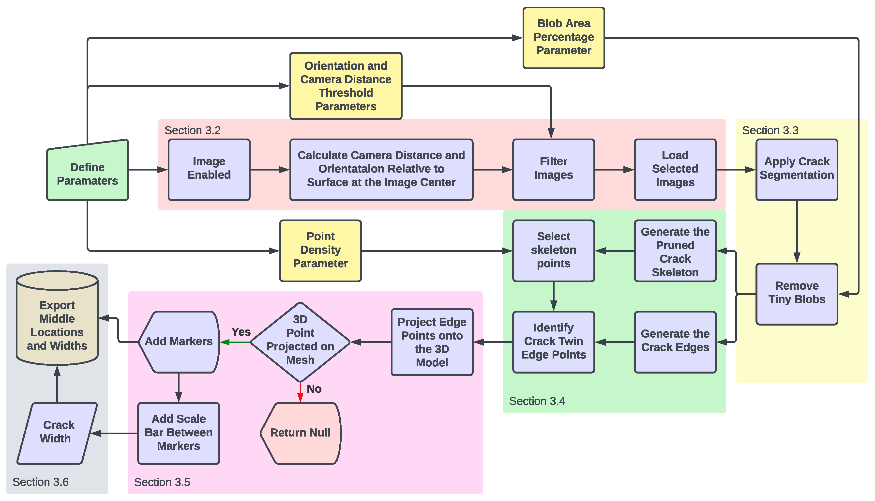
3. Automated Crack Detection and Measurement

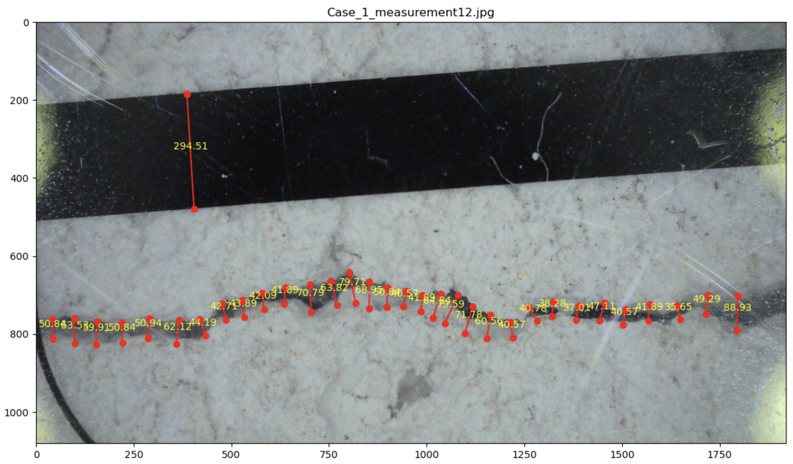
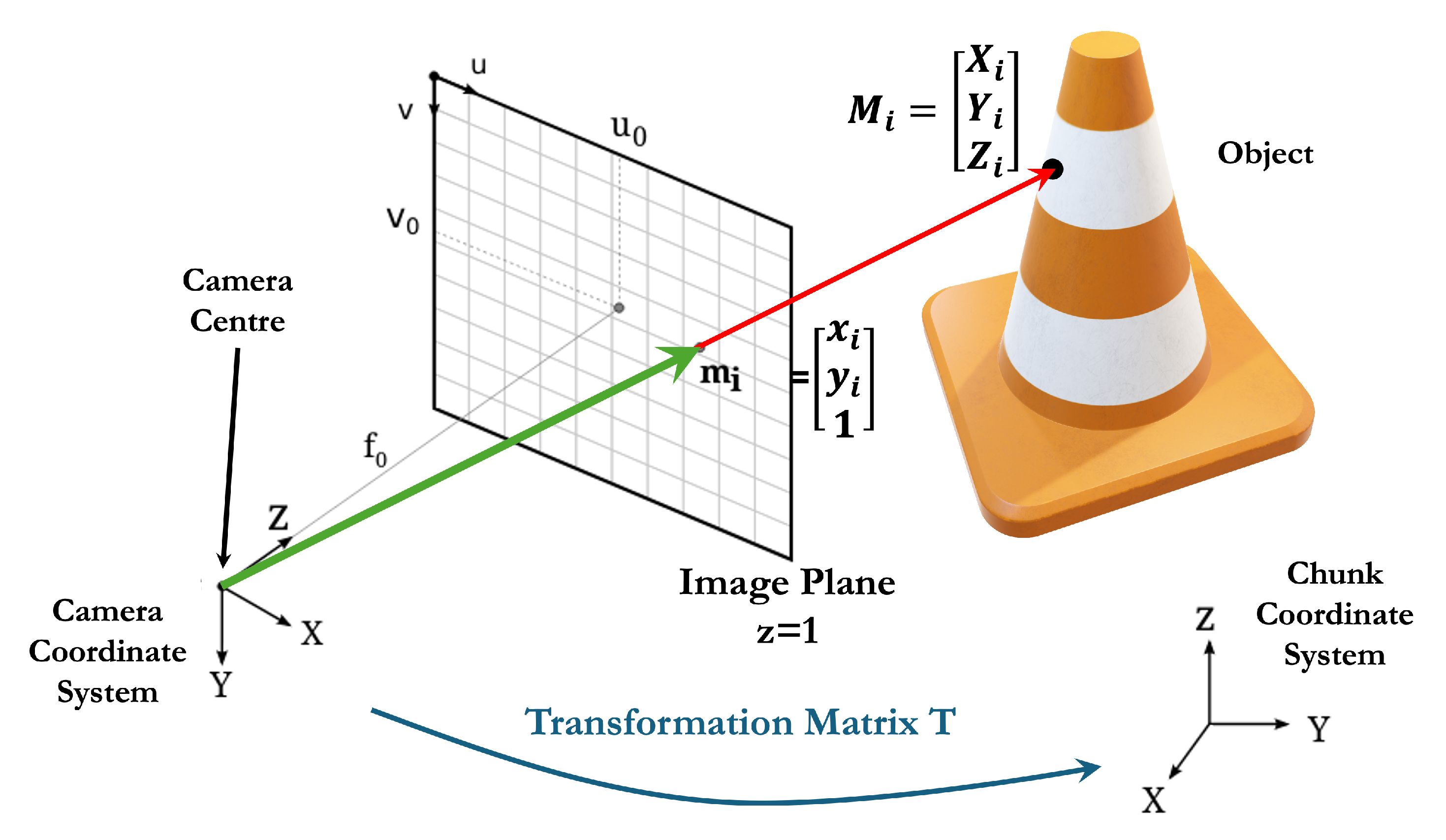
3.1. Crack Detection and Projection Algorithm

The developed Python (Version 3.9.13, suitable version with used Agisoft Metashape API) script introduces a systematic and automated approach for crack detection, segmentation, and measurement within the Metashape environment. Leveraging user-defined parameters, advanced image processing techniques, and 3D point projection, the algorithm streamlines the analysis of cracks in structural surfaces. It provides a robust framework for identifying crack features, measuring their dimensions, and exporting data for further evaluation. This automated solution enhances efficiency and accuracy in structural-health monitoring, offering a reliable tool for crack analysis. An overall flowchart of the system can be seen in Figure 5.

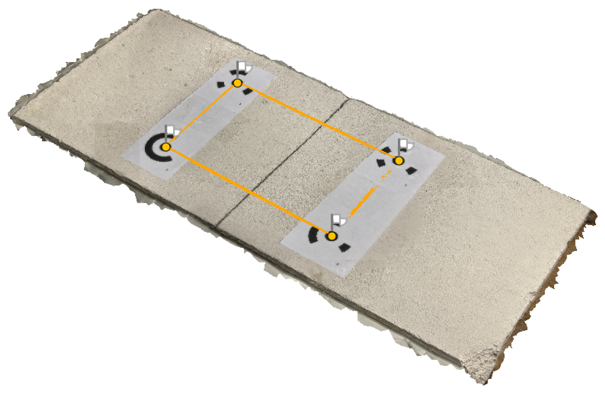
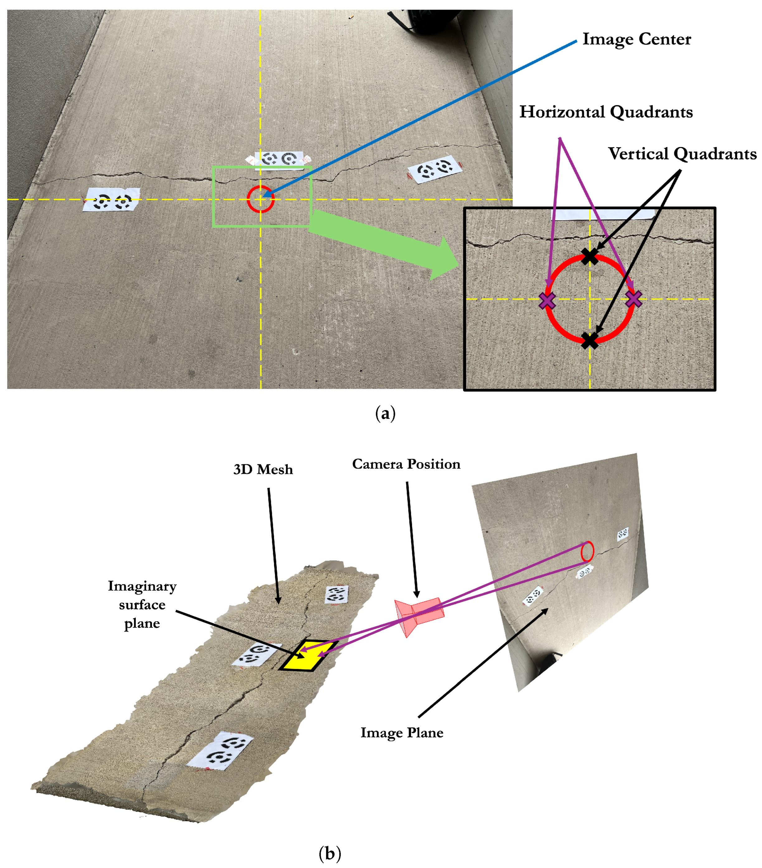
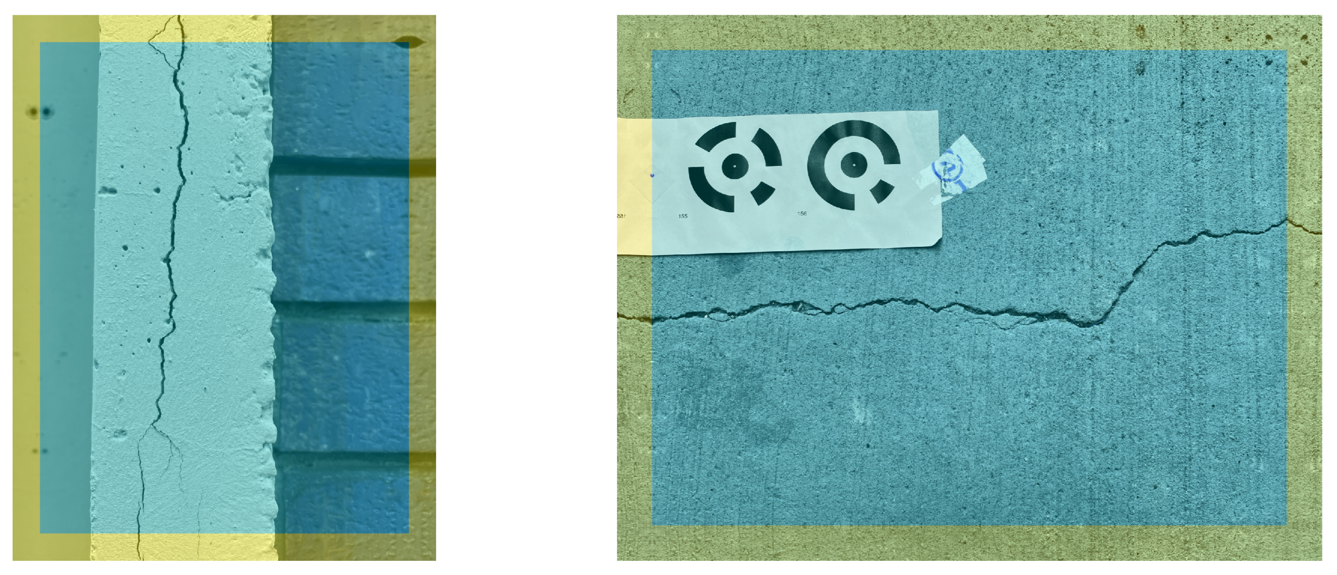
3.2. Camera Selection

In photogrammetry, multiple images are captured from varying distances and orientations to reconstruct a 3D model of an object. However, not all images are suitable for crack detection and width measurement. Images taken from excessive distances often lack the resolution necessary to accurately capture fine crack details, while those not perpendicular to the surface introduce errors in crack detection and projection algorithms. To address these limitations, the proposed methodology selectively utilizes images that are relatively close to the surface and captured orthogonally to it. The optimal values of these two parameters will be researched in Section 4.

Since Metashape does not provide direct tools to determine the relative distance and orientation between the camera and the object’s surface, a custom algorithm was developed and embedded directly into the main processing script. The algorithm calculates these parameters by leveraging the camera positions and orientations computed during the 3D reconstruction process. To estimate the distance, the image center is selected as a reference point. This point is projected onto the 3D surface, with the camera center serving as the first endpoint and the projected point as the second. The Euclidean distance between these two points is then computed to determine the camera-to-surface distance. This process can be seen in Figure 6, and the created geometry is presented in Figure 7.

For orientation estimation, a local surface plane is defined using an imaginary small circle with radius r centered on the image. Four quadrant points on this circle are projected onto the 3D surface using the pinhole camera model, with two points aligned vertically and two horizontally. The distances between the camera center and these projected points are calculated, yielding four distance values per image. Using these distances ($d_1$ and $d_2$) and the camera’s focal length f, two similar triangles are constructed to determine the angle $\theta$ between the camera plane and the surface for each axis, as seen in Figure 7. The orientation angle is derived using geometric relationships and trigonometric functions, as detailed in Figure 6.

$$\left|m\right|=\sqrt{d_1^2+d_2^2-2|d_1\left|\right|d_2|cos\left(2\alpha \right)}$$

(1)

$$\varphi ={\displaystyle \frac{|d_1|sin\left(2\alpha \right)}{2}}$$

(2)

$$\theta =\varphi +\alpha$$

(3)

$$\alpha =arctan\left({\displaystyle \frac{r}{f}}\right)$$

(4)

The smaller of the two orientation angles and the computed distance are used for further analysis. If the projection fails to intersect the 3D mesh, the algorithm returns “−1” for both distance and orientation, prompting the user to decide whether to include or exclude the image.

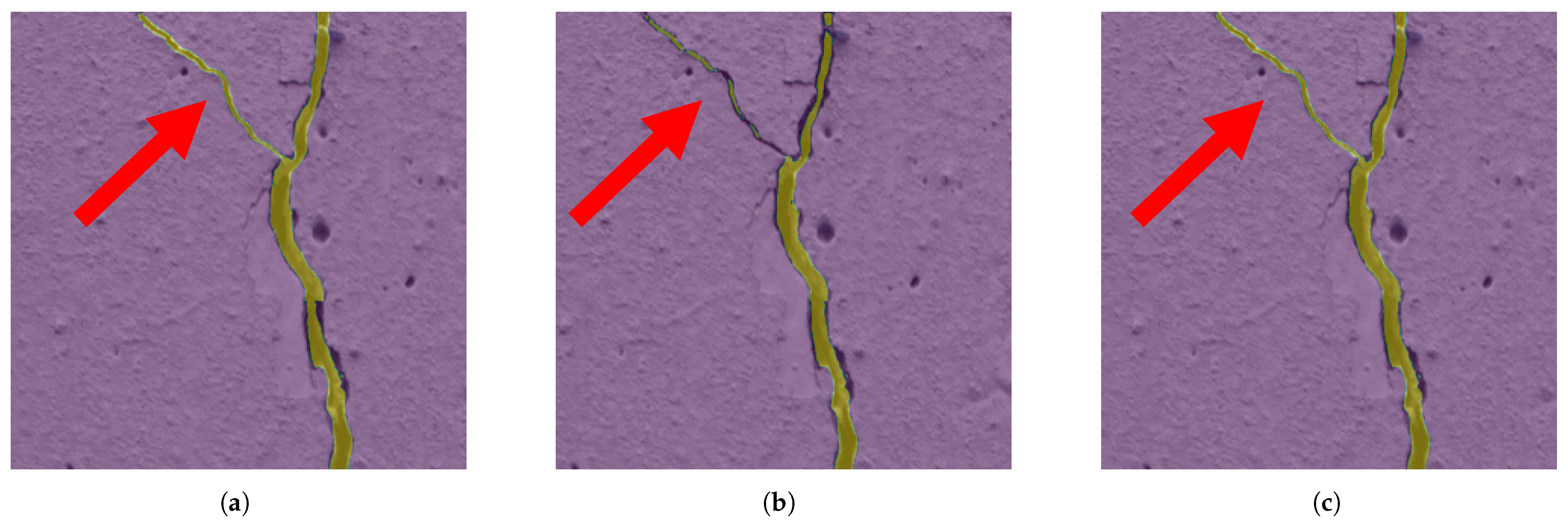
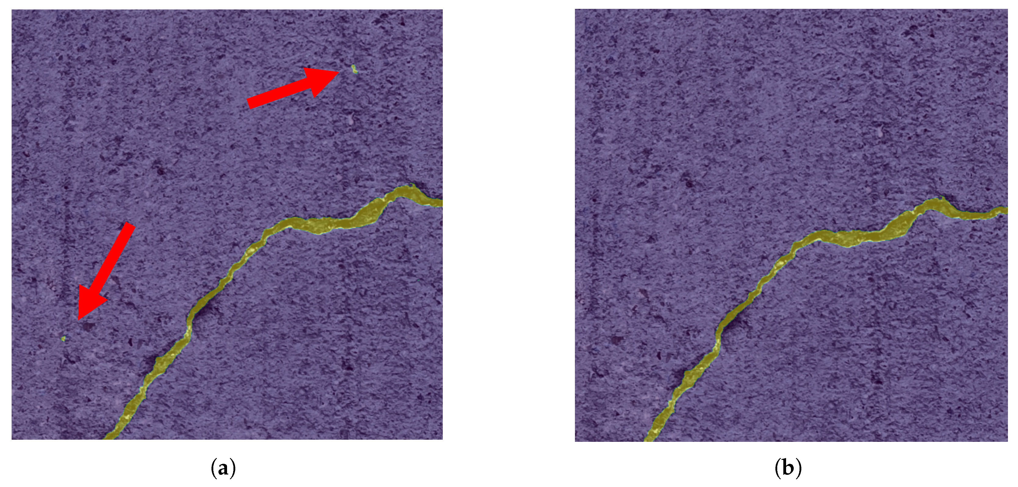
3.3. Binary Crack Segmentation

The core of the crack detection system lies in the automation of crack identification from images, leveraging advancements in the computer vision and machine learning fields. Traditional methods, such as threshold-based techniques (e.g., Otsu’s method) and hand-crafted feature approaches (e.g., morphological operators, wavelet filters), have laid the groundwork for crack detection but face limitations in handling complex crack patterns, uneven lighting, and noise [5]. These methods often require manual intervention and struggle to capture the full variability of crack characteristics.

In contrast, deep learning-based approaches, particularly encoder–decoder CNN architectures like UNet, FPN, PSPNet, and DeepLabV3, have revolutionized crack detection by enabling end-to-end training and multi-scale feature extraction. These models, supported by backbone networks such as ResNet and VGG [20,21], incorporate advanced techniques to achieve precise pixel-level segmentation. Given the need for accurate crack width measurement, which demands pixel-level precision, segmentation models were identified as the most suitable choice for this study.

Segmentation models provide pixel-level precision by delineating the exact boundaries and morphology of cracks. Since this study focuses on crack width measurement, which requires the precise localisation of crack pixels, segmentation models are the most appropriate choice. CNN-based segmentation models are well suited for capturing intricate details and spatial relationships, making them ideal for high-precision tasks such as crack width estimation. Given these requirements, a state-of-the-art crack segmentation model was selected for implementation.

A modified version of a publicly available repository [22], supporting both VGG16 and ResNet101 CNN architectures, can be trained. For this work, ResNet101, with its 101 layers, was selected due to its superior performance on larger datasets [23]. Training was conducted using the publicly available crack datasets seen in

Table 1. List of used crack segmentation datasets in this work.

Dataset Name	Year	Number of Images	Structure Type	Material Type
Crack500 [24]	2019	206	Pavement	Asphalt
Gaps384 [25]	2019	304	Pavement	Asphalt
CFD [26]	2016	118	Pavement	Asphalt
AEL [27]	2016	38	Pavement	Asphalt
CrackTree [28]	2012	68	Pavement	Asphalt
CCIC-600 [29]	2019	30	Bridge	Concrete

, including pavement and concrete crack images, with the latter manually annotated to ensure relevance. Images were resized into 448 × 448 pixels to match the model’s input size. Training was performed on a MacBook Pro with an M1 Pro processor, using default hyperparameters and a batch size of 2 due to memory constraints. The model was trained until no further improvement in validation loss was observed, with the final model selected from epoch 24, as seen in Figure 8.

The pipeline’s modular design will allow the seamless integration of alternative segmentation models in future studies. While ResNet101 was prioritized here for its balance of performance and reproducibility, adopting more advanced architectures could further enhance detection accuracy without requiring systemic changes in the workflow.

The trained model assigns a probability to each pixel, indicating its likelihood of belonging to a crack. Various values were tested, as illustrated in Figure 9, and an optimal confidence threshold of 0.4 was determined to balance crack detection accuracy and avoid over- or underestimation.

Two primary approaches were considered for model inference. The first involves down-sampling images to 448 × 448 pixels, applying the model, and subsequently up-sampling the results to the original dimensions, as seen in Figure 10. While computationally efficient, this method results in loss of detail, often leading to either overestimation or failure to detect cracks. The second approach retains the original image resolution and applies a 448 × 448-pixel sliding window to detect cracks, combining the results into the original image. The window can be overlapped to mitigate detection loss at patch boundaries. In cases of large datasets, non-overlapping processing can be employed for efficiency. Empirical observations indicate that non-overlapping processing also produces satisfactory results, as demonstrated in Figure 11. However, to prevent the fragmentation of cracks at window edges, an overlap of 50% in both the vertical and horizontal directions was selected.

Although overlapping ensures that cracks are not missed, the patching process causes a reduction in crack probability values near the edges, as illustrated in Figure 11. When overlapping is applied, cracks located near image boundaries are often not detected correctly because the model lacks contextual information beyond the patch edges. As a result, the confidence levels for cracks near the borders are lower compared to those in the central regions.

To address this issue, a symmetric padding technique was applied to the original image, matching the size of the overlapping window. This approach involved mirroring the image along its edges and corners, creating a seamless extension of the original content. Specifically, the image was reflected along the top, bottom, left, and right edges, while the corners were padded by mirroring the already extended edges. This ensured that the padded regions provided continuous and consistent contextual information, allowing the model to make more accurate predictions at patch boundaries. Examples of these padded images are shown in Figure 12.

After applying the crack detection model, it was observed that small artifacts, particularly at the object edges, were incorrectly classified as cracks. To eliminate these artifacts, blob removal was applied, removing regions smaller than 0.01% of the total image area, as seen in Figure 13.

The final crack segmentation results on the example images can be seen in Figure 14.

While the patching method effectively captures fine details, its performance declines when segmenting wider cracks or processing low-resolution images. In such cases, it is found that the full segmentation (down-sampled) method yields superior results.

The next critical step involves defining crack edge points and their corresponding twin points to accurately measure crack width. An advanced algorithm proposed in prior research was adapted and integrated into the current system [30].

A crack skeleton was generated using a thinning algorithm by Lee [31], which, when applied directly, often produces unwanted artifacts known as burrs due to the complex geometry of the crack. To address this, the Discrete Curve Evolution (DCE) method [32] was employed to prune these artifacts by simplifying the crack contour. While simplification is necessary for effective pruning, excessive simplification can compromise geometric accuracy. Through trial and error, optimal simplification of level 5 was determined for this study, balancing artifact removal with the preservation of essential geometric details, as seen in Figure 15.

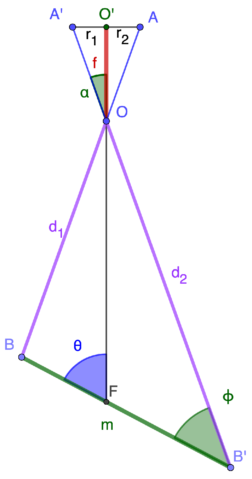
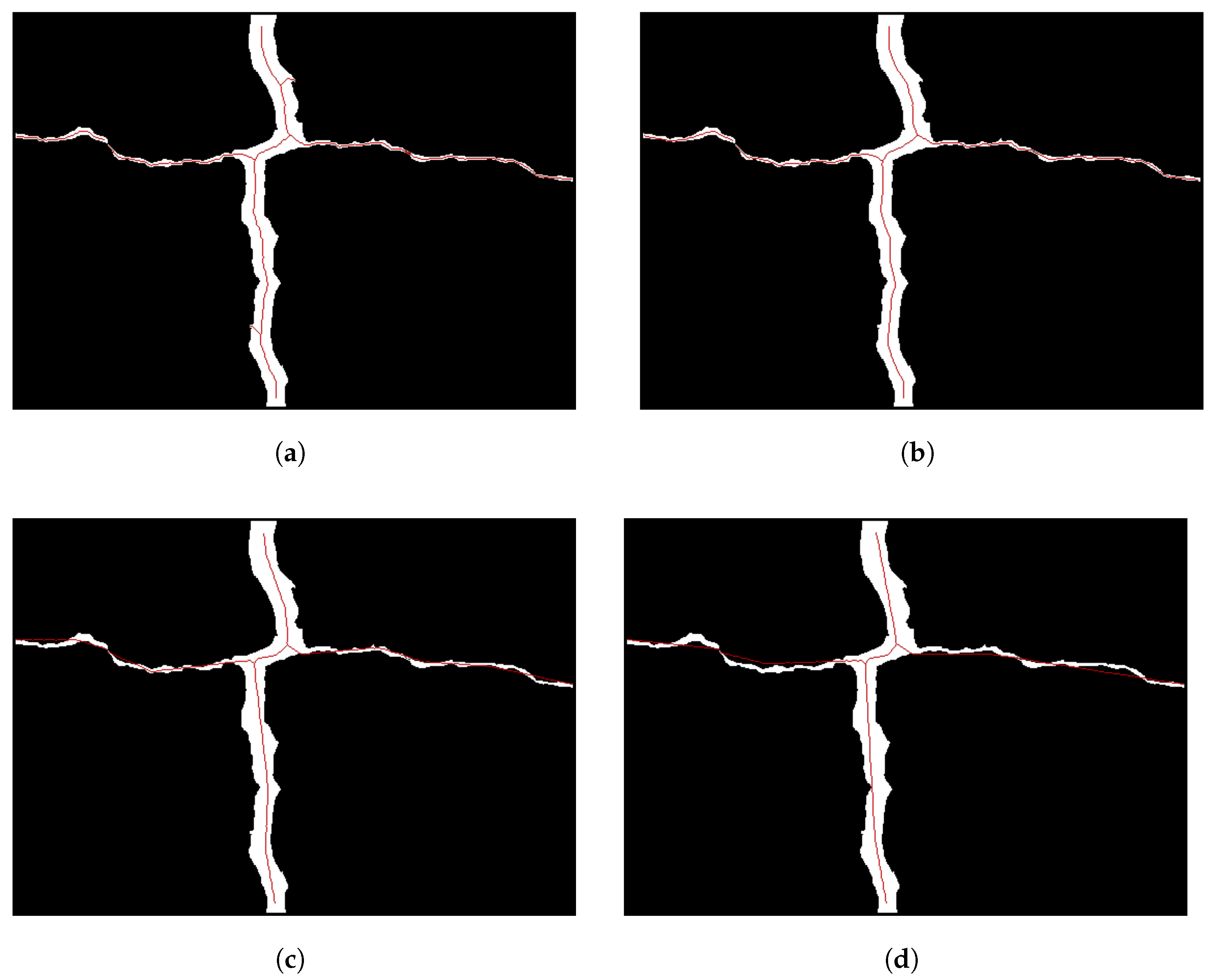
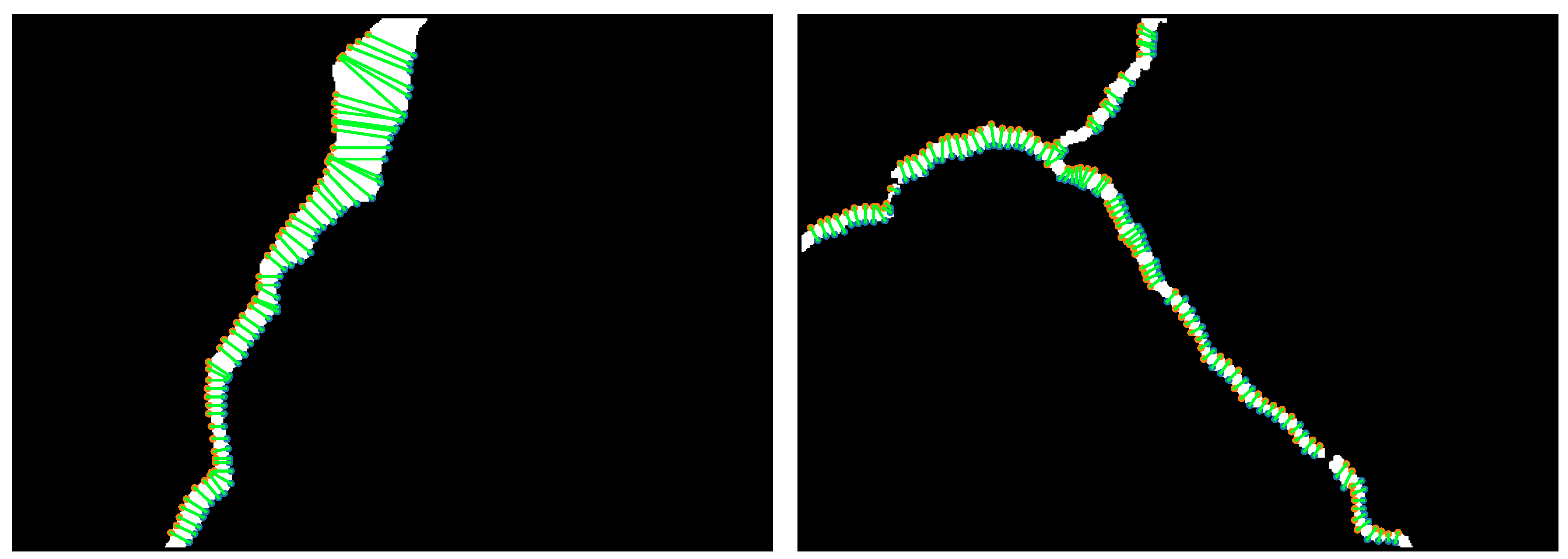
3.4. Selecting Crack Edge Twins

Crack edges were detected using the Canny edge detection algorithm [33]. With both the skeleton and edges identified, twin points representing the crack width were determined using a hybrid approach adapted from [34], which combines two established techniques: the shortest method and the orthogonal method. The shortest method selects edge points closest to the skeleton, while the orthogonal method uses an adaptive window around the skeleton point to identify edges in a direction orthogonal to the skeleton’s propagation.

To handle edge effects, a thin black border was added to the binary image. This border did not interfere with twin point selection, as the algorithm inherently avoided selecting points along these borders due to its reliance on orthogonality. The developed algorithm effectively identifies twin points, as demonstrated in Figure 16.

3.5. Projection of Crack Edges on 3D Mesh Model

A key objective of this study is to utilize 3D width calculations to eliminate distortions caused by non-planar complex surfaces and to determine the 3D position of cracks to obtain a comprehensive understanding of their location within large structures. To achieve this, the twin crack edges identified in the binary image were projected onto the 3D mesh model in Metashape. The overall projection process can be seen in Figure 17.

In Metashape, three surface representations are available for projection: tie points, dense point clouds, and mesh models. Tie points and dense point clouds, while useful for initial reconstruction, represent the object as discrete points, leading to potential inaccuracies in projection. In contrast, the mesh model, composed of small triangular surfaces, allows for the precise selection of any point on the surface, making it the preferred representation for crack edge projection.

The projection process begins by identifying the pixel coordinates (u, v) of the crack edge relative to the image’s top-left corner. These coordinates are undistorted using camera parameters and converted into a 3D point (x, y, z) in the camera coordinate system, with z set to 1. The 3D point is then expressed in homogeneous coordinates to facilitate transformations, including translation and rotation. Metashape internally computes the required transformation matrix, which converts the 3D point from the camera coordinate system to the chunk (world) coordinate system. This conversion can be presented mathematically as

$$\left[\begin{array}{c}u\\ v\end{array}\right]\to \left[\begin{array}{c}x\\ y\\ 1\end{array}\right]\to \left[\begin{array}{c}x\\ y\\ 1\\ 1\end{array}\right]=P_{camera}$$

(5)

$$P_{chunk}=T·P_{camera}$$

(6)

A ray is defined from the camera position through a defined point. Metashape’s built-in function identifies the first intersection of this ray with the mesh surface, corresponding to the projected crack edge point in the 3D model. This process is repeated for both twin crack edges, enabling the identification of corresponding points on either side of the crack. The Euclidean distance between these points, scaled to reflect the actual proportions of the object, provides a measurement of the crack width, which can be seen in the Metashape user interface in Figure 18.

If a crack is detected on the image background (outside the object’s surface), it will not be projected onto the 3D mesh, confirming that the crack is not present on the target object.

3.6. Exporting Results

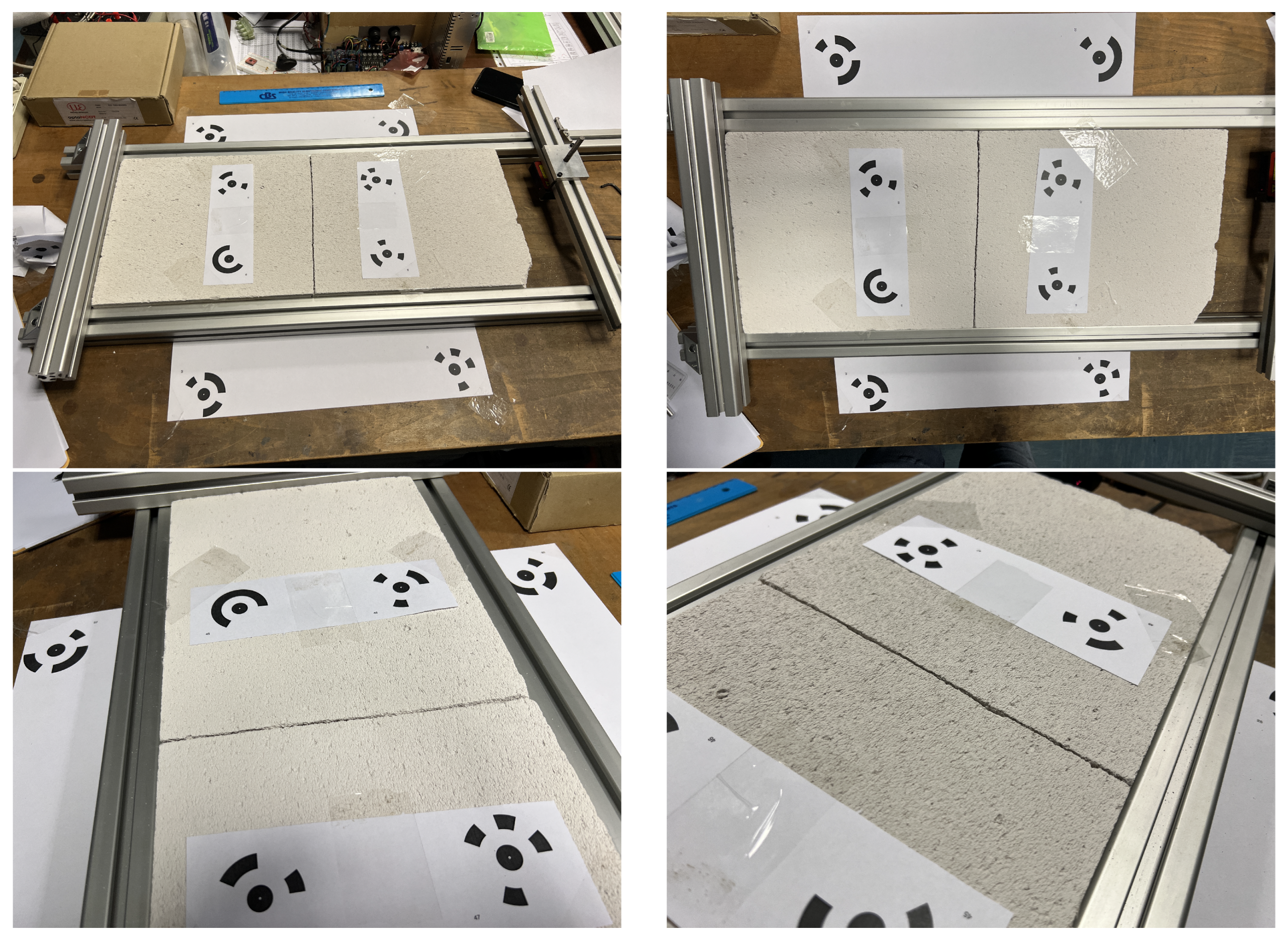
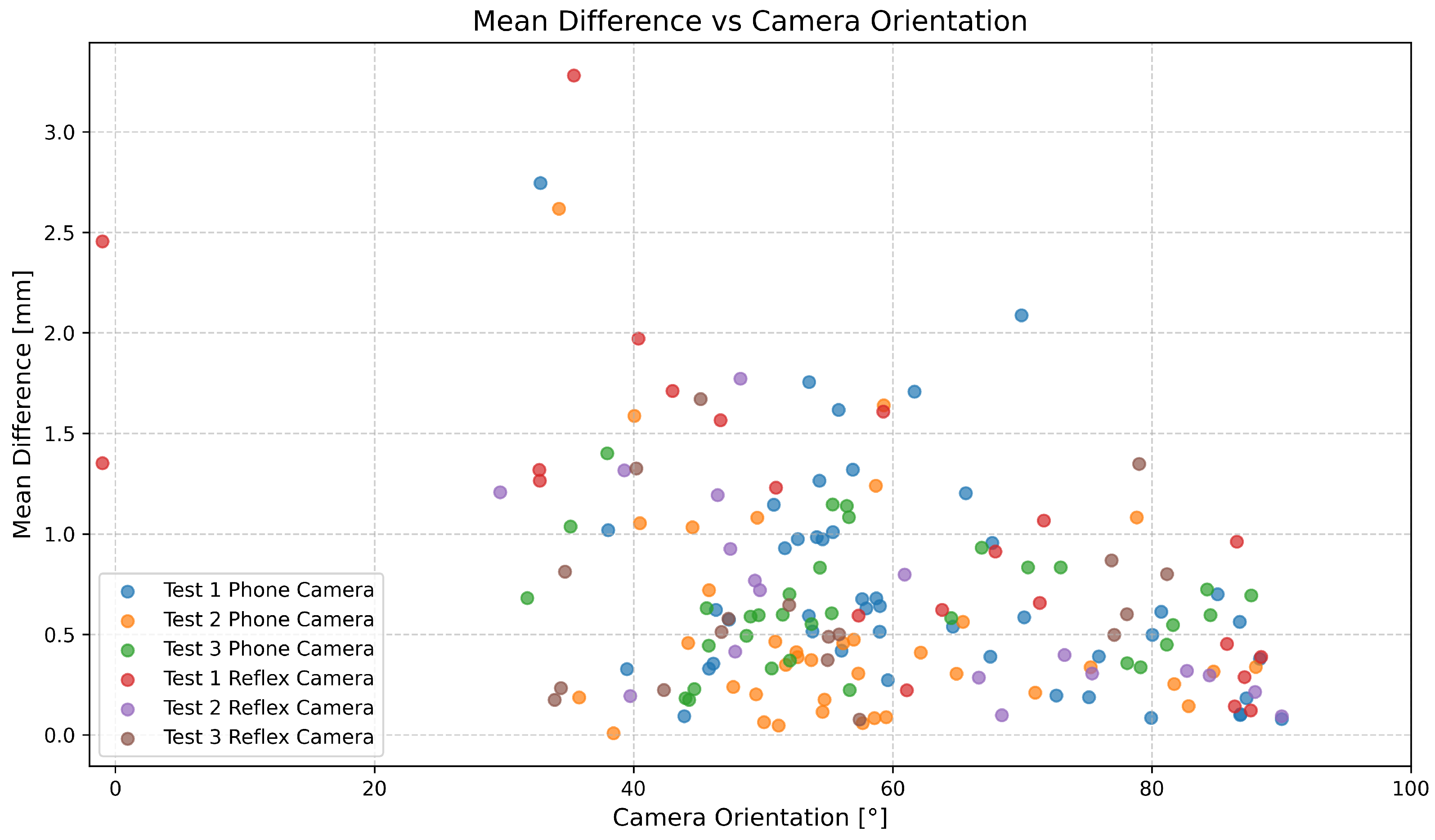
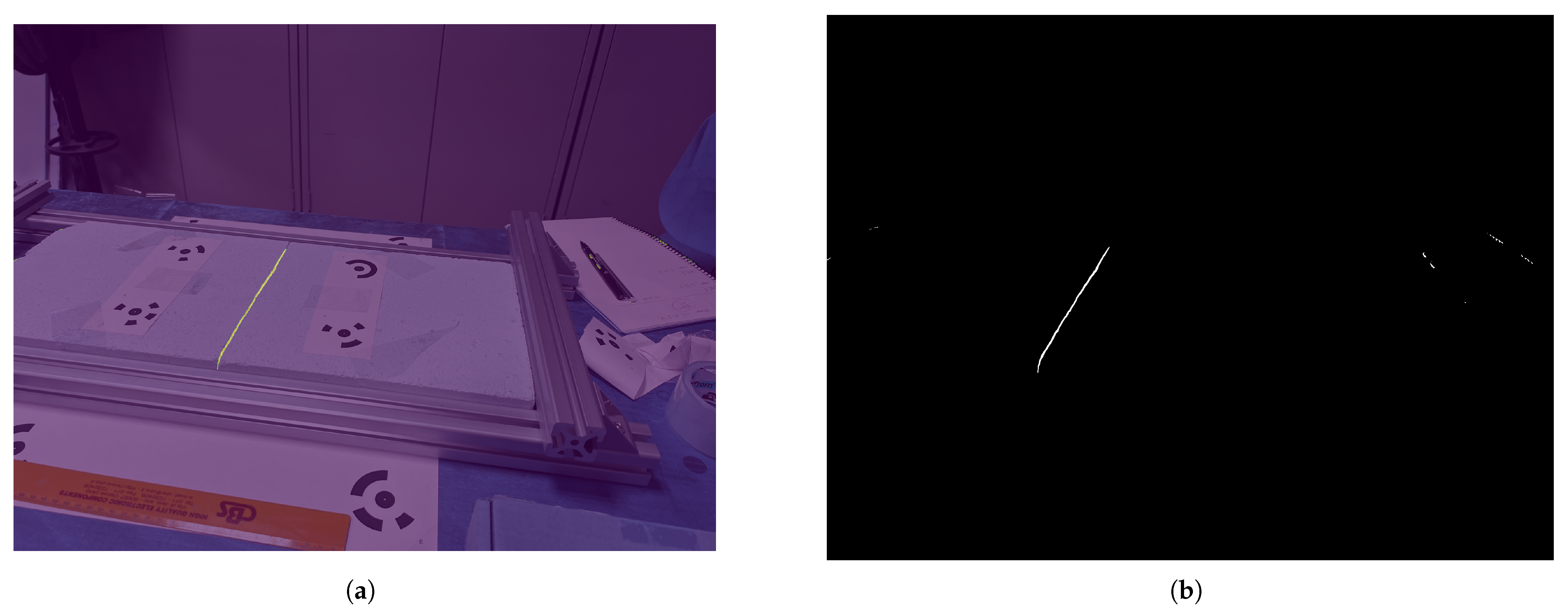
While Metashape excels at photogrammetric processing, its interface lacks optimized tools for crack visualization. The textured mesh (exported as an .obj file with local coordinates) and the Python-generated .txt file of crack midpoints and widths, which are based on same coordinate system, were combined in CloudCompare, enabling the enhanced 3D visualization and analysis of cracks. The example results can be seen in Figure 19.

4. Laboratory Test

To evaluate the crack detection system, lab tests used an Autoclaved Aerated Concrete (AAC) block split centrally to simulate a straight crack. To model varying crack widths, an enclaving skeleton was assembled from aluminum profiles. This skeleton fixed one part of the AAC block while allowing the other part to move with a single degree of translational freedom, as illustrated in Figure 20. This setup enabled the adjustment of the crack width by moving one of the blocks. For this experiment, three different crack widths (w and $\overline{w}$ for average crack width) were considered, as seen in Figure 21. Additionally, a laser distance sensor was attached to measure the displacement of the moving block between tests, providing validation for the manual measurements.

Targets were placed on the AAC block and surrounding desk to ensure accurate scaling of the 3D scene. To evaluate the method’s applicability across camera systems, images were captured using two distinct devices: an iPhone 13 Pro (consumer-grade mobile camera) and a Nikon D5000 (DSLR). Both systems were operated at minimum zoom (fixed focal length) with consistent exposure settings (ISO 64-125, shutter speed 1/100 s) across all tests. Photographs were acquired from various distances and angles with a conservative forward overlap of 90% between successive images, exceeding Metashape’s minimum recommended 60% overlap, to ensure robust photogrammetric reconstruction (example images in Figure 22). The images were processed in Agisoft Metashape to generate 3D scenes, and the proposed crack detection algorithm was applied to analyze the impact of camera orientation and distance on measurement accuracy.

Manual crack measurements were conducted using a microscope camera and a crack gauge, providing a benchmark for comparison. Also, the manual crack measurements were validated by comparing the mean crack width change between different tests with the laser reading deviation. The crack widths were measured at multiple points along the crack, and statistical methods were applied to compare these results with the automated measurements. To align the manual and estimated measurements, Principal Component Analysis (PCA) was used to reduce the three-dimensional positional data of the estimated measurements to a single axis representing crack propagation from 0% to 100%. This alignment allowed for a direct comparison between the manual and estimated measurements along the length of the crack.

The comparison process involved shifting the origin of the estimated measurements to one end of the crack and, in some cases, reversing the dataset to ensure proper alignment with the manual measurements. A general fit between the manual and estimated measurements was expected to validate the adequacy of the estimation. The mean difference between the two datasets was considered as a primary error metric. After confirming a low mean difference, the standard deviation between the manual and estimated measurements was evaluated. An example of a good fit, indicating adequate estimation, is shown in Figure 23.

Since the two cameras used have different intrinsic parameters, the same camera distance for each camera resulted in different spatial resolutions of the crack. To account for this, the camera distance was converted to the ground sampling distance (GSD) using the following formula:

$$GSD={\displaystyle \frac{H·SW}{f·ImW}}$$

(7)

where H is the distance between the camera center and the intersection of the optical axis with the surface, $SW$ denotes the sensor width, f represents the focal length, and $ImW$ is the image width in pixels.

Scatter plots were generated to analyze the relationship between camera orientation, GSD, and mean difference, as shown in Figure 24. The camera orientation plot reveals a trend where lower mean difference errors are associated with camera angles closer to orthogonal (90 degrees) relative to the object surface. Empirically, a filtering criterion can be applied, such as using only images with orientation angles greater than 70 degrees relative to the object surface, to ensure reliable results. Although some acceptable results were observed within the 35-to-70-degree range, these were inconsistent. It was found that the results in these non-orthogonal cases were highly dependent on the crack propagation direction relative to the position and orientation of the camera.

Figure 25, related to GSD, demonstrates a clear trend: a higher spatial resolution (lower GSD values) correlates with lower mean measurement errors.

To determine the optimal GSD range, four images were selected from each test captured with the phone camera, along with one image from Test 2 captured with the reflex camera, all of which yielded adequate results. Using the developed script, the image resolution was reduced (by decreasing the image width in pixels, ImW), which increased the GSD value. The image width ratios relative to the original image were set to 1.0, 0.8, 0.6, 0.5, 0.4, 0.3, and 0.2 to observe the gradual effect.

Since each test had different crack width conditions, the optimal GSD value varied between tests. However, a general optimal range was defined to apply across all tests. The GSD values were selected primarily to ensure low mean difference errors (<0.5 mm). In cases where the mean difference was sufficiently low, the standard deviation difference was also expected to remain low (<0.3 mm). By identifying the lowest and highest GSD values within this range, the minimum and maximum crack width in pixels could be estimated. This can be calculated by dividing the nominal crack width by the GSD, assuming the nominal crack width to be the mean crack width. This approach ensured that the selected GSD values provided consistent and accurate results across all test conditions, as detailed in

Table 2. Adequate GSD regions and corresponding crack widths in pixels.

	GSD [mm/pixels]		Nominal Crack Width [mm]	Crack Width in Pixels
	Lowest Value	Highest Value		Max	Min
Test 1 with Phone Camera	0.05	0.15	0.72	14	5
Test 2 with Phone Camera	0.05	0.17	1.62	32	9
Test 2 with Reflex Camera	0.05	0.27	1.62	32	6
Test 3 with Phone Camera	0.09	0.27	2.41	26	9

.

To accommodate a wider range of conditions, a threshold was defined between 0.09 and 0.15 mm/pixel. This range ensured optimal estimation accuracy across all tests. However, it is possible to use different thresholds depending on the expected crack width.

The results obtained after applying the thresholds are illustrated in Figure 26, where the maximum mean difference error drops less than 1 mm, while average mean difference error is less than 0.5 mm. A comparison between Figure 25 and Figure 26 demonstrates that by implementing the orientation and GSD thresholds, it is possible to pre-select images with the potential to yield more accurate results before executing the proposed system. This pre-selection process enhances efficiency and ensures higher-quality outcomes by filtering out images that are unlikely to meet the desired accuracy criteria.

In Table 2, Test 1 was expected to have a lower minimum GSD value; however, achieving this would require either a high-focal-length camera or capturing images extremely close to the surface. Reducing the camera distance further risked misalignment of the images in the software, making 0.05 mm/pixel the practical limit for the GSD in this test.

According to this Table 2, assuming the mean crack width represents the nominal crack size, a crack must be defined to be around 10 to 30 pixels wide to ensure accurate detection and measurement.

5. Discussion

The proposed crack detection system achieves competitive performance but exhibits limitations, thus requiring further refinement. While its modular design facilitates the integration of alternative segmentation algorithms, its current performance is constrained by the predefined window size for crack analysis, which must be balanced against image resolution and computational resources. Larger cracks exceeding this window or excessively high-resolution images may degrade accuracy, necessitating parameter tuning. Furthermore, validation has thus far been restricted to wall and ground surfaces; scalability to geometrically complex or large-scale infrastructure (e.g., bridges, tunnels) remains untested.

A critical challenge arises from the system’s reliance on orthogonally captured images. Deviations from orthogonal angles introduce geometric distortions between the segmented crack skeleton (e.g., Figure 27) and the physical crack morphology, compromising dimensional precision. This issue is compounded by the inherent loss of 3D spatial context in 2D representations, which complicates angular interpretation—even for human analysts.

Methodological constraints were also identified during validation. Manual measurements, while foundational for benchmarking, introduced errors due to positional shifts between measurement images and the reliance on mean/standard deviation metrics, which overlook crack width distribution. Additionally, spalling and material loss at the crack edges complicated precise manual crack delineation, highlighting the need for automated solutions.

Finally, equipment selection presents a trade-off between usability and performance. Smartphone cameras democratize access for non-experts, whereas DSLR systems yield superior image quality but demand specialized expertise for optimal operation.

6. Conclusions

Structural cracks represent a critical risk to infrastructure integrity, demanding scalable and precise inspection solutions. This study addresses the limitations of traditional methods, including their inefficiency, subjectivity, and inaccessibility, by proposing an automated system integrating photogrammetry (via Agisoft Metashape) with a custom CNN-based crack detection algorithm. The workflow eliminates reliance on specialized hardware, leveraging widely accessible tools and modular design to enhance adaptability across imaging techniques.

The primary novelty of this work lies in its systematic integration of photogrammetry-derived 3D mesh models and camera orientation data for crack width estimation. While individual steps are conventional, their unified implementation into a cohesive, reproducible workflow represents a methodological advancement. The second key contribution is the identification of optimal image selection criteria for photogrammetry. Through methodical testing, we established camera angles (≥70°), working distances, and ground sampling distances (GSDs: 0.09–0.15 mm/pixel) as critical parameters, addressing a gap often overlooked in similar studies.

Validation under controlled conditions demonstrated the system’s accuracy, with optimal performance for cracks measuring 10–30 pixels in width. While parameters such as mesh resolution, camera angle, and ground sampling distance (GSD) were optimized for this study, future work should systematically evaluate their influence across diverse imaging conditions and structural geometries. Further research is also necessary to validate the system’s robustness on full-scale engineering structures with complex crack morphologies (e.g., branching, intersecting, or sub-millimeter cracks). Real-world environments introduce additional challenges such as heterogeneous lighting, occlusions, and irregular surface textures. To address these, the model’s workflow should be deployed on large-scale infrastructure (e.g., bridges, dams, or tunnels) to assess its scalability and adaptability to dynamic field conditions.

References

1. Adhikari, R.S.; Moselhi, O.; Bagchi, A. Image-Based Retrieval of Concrete Crack Properties. Autom. Constr. 2014, 39, 180–194. [Google Scholar] [CrossRef]
2. Yeum, C.M.; Dyke, S.J. Vision-Based Automated Crack Detection for Bridge Inspection. Comput.-Aided Civ. Infrastruct. Eng. 2015, 30, 759–770. [Google Scholar] [CrossRef]
3. Li, G.; He, S.; Ju, Y.; Du, K. Long-distance precision inspection method for bridge cracks with image processing. Autom. Constr. 2013, 41, 83–95. [Google Scholar] [CrossRef]
4. Yang, F.; Zhang, L.; Yu, S.; Prokhorov, D.; Mei, X.; Ling, H. Feature Pyramid and Hierarchical Boosting Network for Pavement Crack Detection. IEEE Trans. Intell. Transp. Syst. 2019, 99, 1–11. [Google Scholar] [CrossRef]
5. Shi, Z.; Jin, N.; Chen, D.; Ai, D. A comparison study of semantic segmentation networks for crack detection in construction materials. Constr. Build. Mater. 2024, 414, 134950. [Google Scholar] [CrossRef]
6. Liu, Y.-F.; Nie, X.; Fan, J.-S.; Liu, X.-G. Image-based crack assessment of bridge piers using unmanned aerial vehicles and three-dimensional scene reconstruction. Comput.-Aided Civ. Infrastruct. Eng. 2020, 35, 511–529. [Google Scholar] [CrossRef]
7. Zhou, L.; Jiang, Y.; Jia, H.; Zhang, L.; Xu, F.; Tian, Y.; Ma, Z.; Liu, X.; Guo, S.; Wu, Y.; et al. UAV vision-based crack quantification and visualization of bridges: System design and engineering application. Struct. Health Monit. 2024, 24, 1083–1100. [Google Scholar] [CrossRef]
8. Ioli, F.; Pinto, A.; Pinto, L. UAV Photogrammetry for Metric Evaluation of Concrete Bridge Cracks. ISPRS Int. Arch. Photogramm. Remote Sens. Spat. Inf. Sci. 2022, 43, 1025–1032. [Google Scholar] [CrossRef]
9. Xu, Z.; Wang, Y.; Hao, X.; Fan, J. Crack Detection of Bridge Concrete Components Based on Large-Scene Images Using an Unmanned Aerial Vehicle. Sensors 2023, 23, 6271. [Google Scholar] [CrossRef]
10. Dung, C.V.; Anh, L.D. Autonomous concrete crack detection using deep fully convolutional neural network. Autom. Constr. 2019, 99, 52–58. [Google Scholar] [CrossRef]
11. Liu, Z.; Cao, Y.; Wang, Y.; Wang, W. Computer Vision-Based Concrete Crack Detection Using U-Net Fully Convolutional Networks. Autom. Constr. 2019, 104, 129–139. [Google Scholar] [CrossRef]
12. Ronneberger, O.; Fischer, P.; Brox, T. U-Net: Convolutional Networks for Biomedical Image Segmentation. In Medical Image Computing and Computer-Assisted Intervention; Springer: Cham, Switzerlan, 2015; Volume 9351, pp. 234–241. [Google Scholar]
13. Yu, C.; Du, J.; Li, M.; Li, Y.; Li, W. An improved U-Net model for concrete crack detection. Mach. Learn. Appl. 2022, 10, 100436. [Google Scholar]
14. Chen, Y.-C.; Wu, R.-T.; Puranam, A. Multi-task deep learning for crack segmentation and quantification in RC structures. Autom. Constr. 2024, 166, 105599. [Google Scholar] [CrossRef]
15. Taheri, S. A review on five key sensors for monitoring of concrete structures. Constr. Build. Mater. 2019, 204, 492–509. [Google Scholar] [CrossRef]
16. Son, T.T.; Nguyen, S.D.; Lee, H.J.; Phuc, T.V. Advanced crack detection and segmentation on bridge decks using deep learning. Constr. Build. Mater. 2023, 400, 132839. [Google Scholar]
17. Golding, V.P.; Gharineiat, Z.; Suliman, H.; Ullah, F. Crack Detection in Concrete Structures Using Deep Learning. Sustainability 2022, 14, 13. [Google Scholar] [CrossRef]
18. Dorafshan, S.; Thomas, R.; Maguire, M. Comparison of deep convolutional neural networks and edge detectors for image-based crack detection in concrete. Constr. Build. Mater. 2018, 186, 1031–1045. [Google Scholar] [CrossRef]
19. Agisoft LLC. Agisoft Metashape User Manual Professional Edition, Version 2.2. Available online: https://www.agisoft.com/pdf/metashape-pro_2_2_en.pdf (accessed on 2 January 2025).
20. Zhou, S.; Canchila, C.; Song, W. Deep learning-based crack segmentation for civil infrastructure: Data types, architectures, and benchmarked performance. Autom. Constr. 2023, 146, 104678. [Google Scholar] [CrossRef]
21. Yang, G.; Liu, K.; Zhang, J.; Zhao, B.; Zhao, Z.; Chen, X.; Chen, B.M. Datasets and processing methods for boosting visual inspection of civil infrastructure: A comprehensive review and algorithm comparison for crack classification, segmentation, and detection. Constr. Build. Mater. 2022, 356, 129226. [Google Scholar] [CrossRef]
22. khanhha. Crack Segmentation. Available online: https://github.com/khanhha/crack_segmentation (accessed on 10 December 2024).
23. He, K.; Zhang, X.; Ren, S.; Sun, J. Deep Residual Learning for Image Recognition. In 2016 IEEE Conference on Computer Vision and Pattern Recognition (CVPR); IEEE: Las Vegas, NV, USA, 2016. [Google Scholar]
24. Zhang, L.; Yang, F.; Zhang, Y.D.; Zhu, Y.J. Road crack detection using deep convolutional neural network. In Proceedings of the 2016 IEEE International Conference on Image Processing (ICIP), Phoenix, AZ, USA, 25–28 September 2016; IEEE: Piscataway, NJ, USA, 2016; pp. 3708–3712. [Google Scholar]
25. Esenbach, M.; Stricker, R.; Seichter, D.; Amende, K.; Debes, K.; Sesselmann, M.; Ebersbach, D.; Stoeckert, U.; Gross, H.-M. How to get pavement distress detection ready for deep learning? A systematic approach. In Proceedings of the 2017 International Joint Conference on Neural Networks, Anchorage, AK, USA, 14–19 May 2017. [Google Scholar]
26. Shi, Y.; Cui, L.; Qi, Z.; Meng, F.; Chen, Z. Automatic Road Crack Detection Using Random Structured Forests. IEEE Trans. Intell. Transp. Syst. 2016, 17, 3434–3445. [Google Scholar] [CrossRef]
27. Amhaz, R.; Chambon, S.; Idier, J.; Baltazart, V. Automatic Crack Detection on Two-Dimensional Pavement Images: An Algorithm Based on Minimal Path Selection. IEEE Trans. Intell. Transp. Syst. 2016, 17, 2718–2729. [Google Scholar] [CrossRef]
28. Zou, Q.; Cao, Y.; Li, Q.; Mao, Q.; Wang, S. CrackTree: Automatic crack detection from pavement images. Pattern Recognit. Lett. 2012, 33, 227–238. [Google Scholar] [CrossRef]
29. Özgenel, Ç.F.; Sorguç, A. Performance Comparison of Pretrained Convolutional Neural Networks on Crack Detection in Buildings. Isarc Proc. Int. Symp. Autom. Robot. Constr. 2018, 35, 1–8. [Google Scholar]
30. Ong, J.C. A-Hybrid-Method-for-Pavement-Crack-Width-Measurement. Available online: https://github.com/JeremyOng96/A-Hybrid-Method-for-Pavement-Crack-Width-Measurement (accessed on 15 November 2024).
31. Lee, T.; Kashyap, R.; Chu, C. Building Skeleton Models via 3-D Medial Surface Axis Thinning Algorithms. CVGIP Graph. Model. Image Process. 1994, 56, 462–478. [Google Scholar] [CrossRef]
32. Bai, X.; Latecki, L.J.; Liu, W. Skeleton Pruning by Contour Partitioning with Discrete Curve Evolution. IEEE Trans. Pattern Anal. Mach. Intell. 2007, 29, 449–462. [Google Scholar] [CrossRef]
33. Canny, J.F. A Computational Approach To Edge Detection. IEEE Trans. Pattern Anal. Mach. Intell. 1986, 8, 679–698. [Google Scholar] [CrossRef]
34. Ong, J.C.; Ismadi, M.-Z.P.; Wang, X. A hybrid method for pavement crack width measurement. Measurement 2022, 197, 111260. [Google Scholar] [CrossRef]
Figure 1. Example image taken on the scene with targets on a concrete surface.
Information 16 00448 g001
Figure 2. (a) Manual crack measurement method used. (b) Crack gauge used.
Information 16 00448 g002
Figure 3. User interface of developed measurement tool for manual crack measurement. Red lines presents the crack width while yellow texts are pixel width values.
Information 16 00448 g003
Figure 4. Example of cleaned textured mesh in Metashape user interface.
Information 16 00448 g004
Figure 5. Overall workflow of developed Python script that runs on Metashape.
Information 16 00448 g005
Figure 6. (a) Surface definition point selection of quadrants on image. (b) Projection of selected points on mesh for vertical case on surface using pinhole camera model.
Information 16 00448 g006
Figure 7. The resulting geometry formed by projecting two quadrants onto an imaginary planar surface.
Information 16 00448 g007
Figure 8. Training and validation loss over epochs.
Information 16 00448 g008
Figure 9. Edge portion of example with different confidence levels: (a) 0.2; (b) 0.4; (c) 0.6. (d) Probability map. In images (ac), yellow regions mean that pixels indicate a crack, and in image (d), yellow regions indicate high confidence and red regions indicate low confidence.
Information 16 00448 g009
Figure 10. Crack segmentation by down-sampling the image to the input size of the model. Yellow regions mean that pixels indicate a crack.
Information 16 00448 g010
Figure 11. Edge portion of example with different confidence levels: (a) no overlap; (b) 50% overlap; (c) 50% overlap with padding. Padding provides better detection around the image boundaries. Yellow regions mean that pixels indicate a crack. Red arrows indicates the area mostly affected.
Information 16 00448 g011
Figure 12. Example of padded images. Yellow region is padded part while cyan region is original part of image.
Information 16 00448 g012
Figure 13. The cleaningprocess with blob removal on an example. (a) The initial result of the model; (b) the cleaned result. Yellow regions mean that pixels indicate a crack. Red arrow indicates the removed blobs.
Information 16 00448 g013
Figure 14. (ac) Examples of crack images. (df) Corresponding crack segmentation respectively.
Information 16 00448 g014
Figure 15. Different simplification levels with Discrete Curve Evaluation: (a) original skeleton with burrs, (b) DCE simplification level 5, (c) DCE simplification level 10, and (d) DCE simplification level 15. Red line denotes estimated crack skeleton.
Information 16 00448 g015
Figure 16. Examplesof crack twins (green lines) selected using proposed method.
Information 16 00448 g016
Figure 17. Proposed projection process in Metashape.
Information 16 00448 g017
Figure 18. Estimated crack edges and widths in Metashape UI (user interface). (a) Selected crack twin edges on image. (b) Projected crack twin edges on mesh. Points with blue or white flags represent crack edge, while yellow lines between flags denote crack width.
Information 16 00448 g018
Figure 19. Example of detected cracks in CloudCompare user interface.
Information 16 00448 g019
Figure 20. Test setup used in experiment.
Information 16 00448 g020
Figure 21. Portion of cracks on three different tests: (a) Test 1, w ¯ = 0.74 mm; (b) Test 2, w ¯ = 1.62 mm; (c) Test 3, w ¯ = 2.41 mm.
Information 16 00448 g021
Figure 22. Example images taken in scene for photogrammetry and crack detection application.
Information 16 00448 g022
Figure 23. Example of good fit between manual measurements and estimated measurements: (a) comparison between positions along crack; (b) comparison of histograms.
Information 16 00448 g023
Figure 24. Scatter plot of mean difference vs. camera orientation for all tests.
Information 16 00448 g024
Figure 25. Scatter plot of mean difference vs. GSD for all tests.
Information 16 00448 g025
Figure 26. Threshold-applied scatter plot of mean difference vs. GSD for all the tests.
Information 16 00448 g026
Figure 27. (a) Non-orthogonal image example with detected crack in yellow. (b) The corresponding segmentation.
Information 16 00448 g027