Abstract
In feature selection, it is crucial to identify features that are not only relevant to the target variable but also non-redundant. Conditional Mutual Information Nearest-Neighbor (CMINN) is an algorithm developed to address this challenge by using Conditional Mutual Information (CMI) to assess the relevance of individual features to the target variable, while identifying redundancy among similar features. Although effective, the original CMINN algorithm can be computationally intensive, particularly with large and high-dimensional datasets. In this study, we extend the CMINN algorithm by parallelizing it for execution on Graphics Processing Units (GPUs), significantly enhancing its efficiency and scalability for high-dimensional datasets. The parallelized CMINN (PCMINN) leverages the massive parallelism of modern GPUs to handle the computational complexity inherent in sequential feature selection, particularly when dealing with large-scale data. To evaluate the performance of PCMINN across various scenarios, we conduct both an extensive simulation study using datasets with combined feature effects and a case study using financial data. Our results show that PCMINN not only maintains the effectiveness of the original CMINN in selecting the optimal feature subset, but also achieves faster execution times. The parallelized approach allows for the efficient processing of large datasets, making PCMINN a valuable tool for high-dimensional feature selection tasks. We also provide a package that includes two Python implementations to support integration into future research workflows: a sequential version of CMINN and a parallel GPU-based version of PCMINN.
1. Introduction
In recent years, we have witnessed the phenomenon of big data, with data continuously growing due to various factors such as the rapid development of technology, the widespread use of the internet, and the rise of interconnected devices [1,2]. The advent of big data has brought an unprecedented increase in the dimensionality of datasets, particularly in domains such as genomics, image analysis, speech recognition, financial modeling and cybersecurity [2,3,4]. It is now common to encounter datasets with thousands of variables and extremely high dimensionality [5]. For example, data from the popular LIBSVM repository, such as the KDD2010 dataset, demonstrate this trend, with approximately 20 million samples and 29.8 million features, indicating a significant increase in data scale and complexity [6]. These data become particularly valuable when they enable us to gain insights that guide future decisions or support evidence-based conclusions [7]. However, as the complexity and the size of data increase, so do the challenges related to its analysis and processing [8]. High-dimensional data pose several challenges to machine learning algorithms, including the curse of dimensionality, increased model complexity, overfitting and high computational cost [9,10]. This often leads to computationally expensive analyses and, in some cases, to less reliable conclusions due to the presence of redundant or irrelevant features. For researchers and engineers in the field of data mining, this has become a critical issue, especially when they try to extract useful information, knowledge and patterns from such large-scale datasets [11].
In the age of big data, the field of data mining has become essential, because it enables the extraction of valuable insights from large and complex datasets. Fundamentally, data mining is the process of extracting useful information [12], such as dependencies and patterns that are not immediately apparent [13]. It encompasses a number of processes [14], including data formatting and cleaning, database development, data visualization and also feature selection, which is the primary focus of the present study.
As previously mentioned, some algorithms struggle when processing datasets that are large both in terms of the number of features and the number of samples [15]. Therefore, adapting existing methods becomes essential to ensure efficiency and effectiveness. To address the challenges posed by high-dimensional data, dimensionality reduction techniques are commonly employed to reduce the number of features and enhance the performance of machine learning models [16,17]. One of the most popular methods among these approaches is feature selection [18]. Feature selection is often used as a preparatory stage of machine learning or in conjunction with it [19]. Rather than transforming the original features, feature selection methods work by identifying and removing those that are irrelevant or redundant, thereby simplifying the model, while preserving interpretability [20]. Due to this, feature selection methods are considered particularly valuable in fields where drawing insightful conclusions or understanding model decisions is essential [21].
Feature selection techniques can be classified into four categories: filters [22,23], wrappers [24,25], embedded approaches [26,27], and hybrid approaches [28,29]. Among these, filter methods are often preferred in large-scale applications, as they are typically unsupervised and computationally efficient. Within filter methods, the approaches that employ information theory measures for identifying feature relevance have attracted considerable attention, due to their ability to detect both linear and nonlinear dependencies [30]. These methods rank features based on their mutual information with the target variable [31], while also taking into account redundancy with features that have already been selected [32].
However, traditional mutual information (MI)-based approaches, such as mRMR [33] and MIFS [34], rely on simplifying assumptions. They typically use pairwise mutual information, which does not adequately capture higher-order dependencies or conditional interactions. Moreover, many MI estimators, especially those based on discretization (binning), suffer from bias and sensitivity to parameter choices, particularly in high-dimensional continuous spaces [35]. Note that mRMR’s criterion involves only the terms and and thus cannot account for combined effects among features in the selected subset S, often leading to suboptimal results. This limitation also applies to MIFS, which similarly relies on pairwise approximations. In contrast, the Conditional Mutual Information Nearest-Neighbor (CMINN) method [36] is more general-purpose than other MI filters in that it considers the relevance of two or more features in S jointly with the class variable or the candidate feature.
CMINN addresses many of these limitations by employing a non-parametric k-nearest-neighbor (kNN) estimator of conditional mutual information [37]. It performs a sequential forward feature selection based on the conditional mutual information between each candidate feature and the class label, conditioned on the set of features already selected. Unlike its predecessors, CMINN evaluates the relevance and redundancy of features within a unified framework, enabling the detection of synergistic interactions among features and improving selection performance in complex, high-dimensional settings.
While CMINN offers strong theoretical foundations and demonstrates improved performance over traditional MI-based methods, it comes with a significant computational cost. Specifically, the repeated estimation of conditional mutual information using high-dimensional k-nearest-neighbor searches and local density computations introduces substantial overhead. As the number of features and instances increases, the complexity of these operations grows rapidly, making the direct application of CMINN to large-scale datasets computationally demanding. This limitation poses practical challenges in domains where speed and scalability are critical, highlighting the need for further optimization or approximation strategies [38].
In this paper, we present a GPU-accelerated version of the CMINN algorithm that significantly reduces runtime, while preserving its core algorithmic structure. By leveraging high-level GPU libraries such as CuPy and cuML, we implement a parallelized variant of CMINN that executes efficiently on NVIDIA GPUs. Our results in the following simulation study demonstrate that substantial speedups can be achieved using general-purpose GPU computing in Python, even without resorting to custom CUDA kernel development. In addition, we detail the architectural design, implementation choices and performance characteristics of our approach and we also highlight potential paths for further acceleration through low-level CUDA optimization as in [39,40,41].
Specifically, we present the following novel aspects:
- A GPU-accelerated version of the CMINN algorithm (PCMINN), designed to handle large-scale, high-dimensional datasets efficiently.
- A full implementation in Python using CuPy and cuML, offering accessibility and full GPU residency without requiring CPU–GPU data transfers.
- A comprehensive experimental evaluation including synthetic and real-world datasets, as well as analysis of execution time, ranking consistency and parameter effects.
- The release of a publicly available implementation to support reproducibility and further adoption of information-theoretic feature selection methods.
The rest of the paper is organized as follows: In Section 2, basic elements of the relevant theory, as well as the methodology followed, are presented. In Section 3, a simulation study conducted on three different datasets is described, while Section 4 and Section 5 provide the discussion and our conclusions, respectively.
2. Materials and Methods
In this section, the tools and methods that were used are described. Initially, some theoretical background on mutual information and conditional mutual information is described. Next, the CMINN model and the proposed parallel implementation are presented.
2.1. Information Theory Measures
2.1.1. Mutual Information Estimation
Mutual information (MI) [42] measures the amount of information that two random variables share and, specifically, how much uncertainty about one variable is reduced when the other variable is known. It is an entropy-based measure that detects both linear and nonlinear dependencies. For continuous random variables X and Y, the information one variable carries about the other and vice versa is measured by
where is the joint probability of X and Y, whereas and are their marginal probabilities, respectively. For discrete variables, the integral becomes a summation over the joint and marginal probability mass functions.
For discrete variables, the estimation of MI is straightforward, while for continuous ones, a free parameter depending on the chosen estimator has to be determined. For example, for the binning estimator, a parameter b has to be defined, which determines the number of cells into which the domain has to be divided. Nevertheless, the value of b has been correlated with the size of bias, since it has been observed that the larger the b, the greater the bias [35]. However, in some cases, it is necessary to have a larger value of b in order to resolve complex dependencies between variables and, at the same time, a smaller bias is also preferable [43]. Due to this, some nonparametric methods for density estimation such as nearest-neighbors, B-splines [44], and kernels [45], which have been found to be less sensitive to their free parameter [46] and also less sensitive to data size, are preferred compared to the binning one.
In this work, the nearest-neighbor method is used for the estimation of both mutual information and conditional mutual information. Specifically, the Kraskov–Stögbauer–Grassberger (KSG) estimator is employed [37], which expresses mutual information in terms of distances to the k-th nearest-neighbors and digamma functions:
where N is the number of samples, is the digamma function and and are the number of neighbors within the i-th point’s local radius along the X and Y marginal spaces, respectively. To be precise, we will analyze this a little bit further.
In the nearest-neighbor-based estimation of mutual information, for each data point i, we compute the distance to its k-th nearest-neighbor in the joint space of the variables . This distance () defines a local neighborhood around point i. Then, for each marginal space X and Y and for each i, we examine how many data points (including itself) fall within a distance less than . The number of neighbors is denoted as and , respectively. These local counts are then used to estimate mutual information, exploiting the relationship between joint and marginal densities. It has to be noted that this assessment of mutual information can be applied for vector variables X and Y of any dimension, since it is independent of the data scale and depends only on the local densities. This estimation of mutual information is found to be less sensitive to data size and also to its free parameter k [35,46].
2.1.2. Conditional Mutual Information Estimation
To mitigate redundancy among features, conditional mutual information (CMI) is used. It extends mutual information (MI) by measuring the mutual dependence between X and Y, given a third variable Z:
where denotes differential entropy. Intuitively, CMI quantifies the amount of information X provides about Y beyond what is already explained by Z. This is what makes it particularly relevant for feature selection, where the aim is to add to the optimal feature subset a new candidate feature that contributes novel information beyond the already known. Additionally, the advantage of CMI is that it has reduced bias in comparison with MI, since its bias is essentially the difference of the bias of the two MI terms.
Similar to MI, we compute CMI using the same nearest-neighbor approach:
where , and give the number of points whose distance from the i-th point in the projected spaces of , and Z, respectively, is less than . refers to the distance of the i-th sample point from its k-th nearest-neighbor in the joint space .
It has to be noted that conditional mutual information estimated by this method has been shown to have low bias for large dimensional datasets [47]. However, it requires the computation of nearest-neighbors in multiple subspaces at every iteration of the feature selection algorithm—an expensive step, especially when the number of candidate features or dimensionality of Z is large.
2.2. CMINN Feature Selection Algorithm
CMINN (Conditional Mutual Information Nearest-Neighbor) [36] is a feature selection algorithm that uses conditional mutual information (CMI) estimated via nearest-neighbor in order to create the optimal subset of features that best describe the class variable.
Given a dataset with M candidate features and a class variable C, the goal is to identify a subset that contains the most informative and least redundant features with respect to C. CMINN builds S incrementally through a greedy, forward-selection process:
- Initialize the selected feature set S = Ø.
- Select the first feature as the one that maximizes mutual information with the classand set .
- At each subsequent iteration, compute the conditional mutual information between each remaining feature and the class variable, conditioned on the current set of the already selected features S:The feature with the highest conditional information is added to S.
- Repeat step 3 until a termination condition is met or a predefined number of features has been selected.
The criterion in step 3 takes into account both relevance and redundancy. Basically, the feature should provide useful information about the class C (relevance), but it should not repeat information that is already captured by the features in S (redundancy). This balance helps avoid selecting overlapping features. Since the nearest-neighbor-based estimator can handle multiple features in S, CMINN works well even with complex and high-dimensional datasets.
In the original version of CMINN, a stopping criterion was introduced to check whether adding a new feature actually leads to a meaningful increase in mutual information with the class variable. However, in this study, we did not use it, but instead we set the number of features at which we wanted the algorithm to stop, since the efficiency of the termination criterion has been examined in the original publication and our study here focuses purely on comparing the original CMINN with its parallel variant concerning their ability to find the optimal feature subsets and their execution times.
2.3. PCMINN
As aforementioned, despite conditional CMI demonstrating low bias for large dimensional datasets, it requires the computation of nearest-neighbors in multiple subspaces at every iteration of a feature selection algorithm, which is computationally expensive, especially when the number of candidate features or dimensionality of Z is large. While CMINN is considered effective in finding the optimal subset of features, its structure and the continuous nearest-neighbor searches make it computationally expensive, especially in high-dimensional problems. To overcome this bottleneck, we propose a GPU-accelerated implementation, termed PCMINN, which leverages parallel computation for efficient feature evaluation.
PCMINN follows the same greedy forward-selection structure as CMINN, but executes the entire feature selection process on GPU. All array operations are performed using CuPy, while nearest-neighbor searches required for estimating mutual and conditional mutual information are accelerated using cuML’s NearestNeighbors. This fully GPU-based design enables high-throughput computation, especially in high-dimensional settings [40]. Our current implementation leverages high-level GPU libraries such as CuPy and cuML for parallel computation and nearest-neighbor search, prioritizing accessibility and ease of adoption over low-level manual control. Consequently, the parallelization strategies (e.g., thread scheduling, memory access optimization) are handled internally by cuML’s NearestNeighbors implementation, which uses batched brute-force distance computations across GPU cores. The selection loop (based on maximizing conditional MI) iteratively updates the feature subset using GPU-native tensor operations. The GPU workload is structured to keep all distance matrix operations and neighbor counting inside the device, minimizing data movement. We further optimized memory usage using CuPy’s memory pool and controlled batch sizes, which prevented out-of-memory errors. Unlike traditional CPU-based implementations that handle all computations sequentially, PCMINN splits the workload between CPU and GPU. CPU is responsible for initializing the pipeline, generating and normalizing the dataset and managing overall control flow. Once the dataset is prepared, it is transferred to GPU, where all computation-intensive operations, including distance computations and mutual information estimation, are executed. This division of labor allows for significant speedups, while keeping memory operations optimized.
Figure 1 illustrates the interactions between the CPU, GPU and key libraries throughout the PCMINN pipeline.
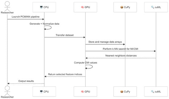
Figure 1.
Interaction diagram of PCMINN pipeline across CPU, GPU, CuPy and cuML components. The CPU handles preprocessing and coordination, while the GPU executes the core computations.
It is worth noting that the original CMINN implementation employs a KD-tree structure to speed up nearest-neighbor queries in CPU-based computation. In contrast, on GPU, PCMINN uses a brute-force approach to compute all pairwise distances. To keep all data and computation on the GPU and avoid the significant overhead of data transfers between CPU and GPU, we opted for brute-force neighbor search, which is fully supported by the cuML library. Although more advanced GPU-based structures such as FAISS could potentially accelerate neighbor search, they do not natively support CuPy arrays and would have required frequent memory transfers or conversions. Similarly, KD-tree implementations are not optimized for GPU execution and are less effective in high-dimensional spaces. Thus, brute-force was the most compatible and efficient option for our fully GPU-resident design. Although brute-force has higher theoretical complexity, the massive parallelism of GPUs offsets this cost and makes it more efficient in practice for high-dimensional data. However, in lower-dimensional cases, the CPU-based KD-tree search may still be faster due to its logarithmic scaling and reduced overhead.
At each iteration, PCMINN evaluates all remaining candidate features by computing their conditional mutual information with the class variable C, given the already selected subset S. The candidate feature with the highest CMI is added to S and the process repeats until a pre-fixed number of features is selected. Unlike the original CMINN, we omit the stopping criterion in this version to enable fixed-budget selection and simplify benchmarking.
To ensure robustness and mitigate numerical issues, we apply min–max normalization to input features and add small noise perturbations when necessary. In the simulation study, additive noise was introduced to evaluate the robustness of the feature selection algorithms under more realistic, non-ideal conditions. The rationale for introducing noise is to simulate real-world conditions where features are often noisy due to measurement imperfections or environmental variability. Evaluating how feature selection methods behave under such perturbations provides insight into their stability and reliability. From a theoretical standpoint, as discussed in the original CMINN paper, the nearest-neighbor estimator of mutual and conditional mutual information is formally designed for continuous random variables. In feature selection, however, the class variable is typically discrete. This can lead to issues such as the accumulation of identical values along certain dimensions in the joint space, which affects distance calculations and neighbor counts. A partial remedy proposed in the original paper is to add an infinitesimal amount of noise to each discrete value. In our case, however, we treated the class variable as discrete without adding noise, which interestingly led to improved results. This is kind of the opposite problem that binning estimates of MI and CMI have, discretizing continuous-valued features. In spite of this apparent shortcoming of the NN estimate in the presence of discrete-valued features, we were able to obtain stable results in all simulations. Despite this known limitation, the method produced stable results across all our experiments.
The implementation is fully batched and parallelized, enabling the selection of informative feature subsets even in datasets with hundreds of features and thousands of samples. The full PCMINN pseudocode is described in Algorithm 1.
| Algorithm 1 PCMINN: GPU-Accelerated Feature Selection |
| Require: Feature matrix , class vector , number of features to be selected d, number of neighbors k |
| Ensure: Selected feature indices S |
| 1: Initialize |
| 2: Let F be the set of all feature indices |
| 3: for to d do |
| 4: for all (in parallel on GPU) do |
| 5: Compute using Kraskov k-NN estimator |
| 6: end for |
| 7: |
| 8: |
| 9: end for |
| 10: return S |
2.4. Experimental Workflow and Implementation Details
The experimental pipeline simulates three synthetic datasets:
- Dataset A: Multivariate Gaussian data with a fixed correlation coefficient (); the response is a weighted sum of two latent target variables.
- Dataset B: Linearly and nonlinearly transformed Gaussian features introducing interactions among subsets of variables.
- Dataset C: Includes informative, redundant and noise features using controlled block structures and interaction terms.
Each dataset contains 10,000 instances and 22–30 features, depending on the type. For each configuration, the pipeline runs 10 iterations using random seeds from 5 to 14. During preprocessing, features are scaled to the range and the response variable is discretized into b bins using equal-width binning. This binning step converts the continuous target into a pseudo-discrete variable, suitable for neighbor-based mutual information (MI) estimation.
The number of features to be selected per dataset is predefined: 5 for Dataset A, 4 for Dataset B and 6 for Dataset C. For each run, PCMINN selects this number of features using CMI-based forward selection. Execution time and selected feature indices are logged. Results are saved in two CSV files, one for per-run execution times and another for the selected features and their associated MI/CMI scores. Regarding the impact of the neighborhood parameter k, we rely on the original CMINN study [36], which systematically explored multiple values (e.g., k = 1, 5, 10, 20, 40) across diverse data structures and sample sizes. Their findings demonstrated that the choice of k does not significantly affect feature selection outcomes or classification performance, as long as it remains within a reasonable range.
Figure 2 summarizes the full simulation loop used for this study.
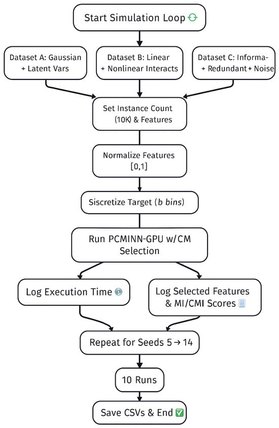
Figure 2.
End-to-end simulation loop for the PCMINN evaluation across Datasets A, B and C. Each run includes normalization, binning, fixed feature selection, execution timing and result logging over 10 iterations.
2.5. Computational Environment
All experiments were performed on a high-performance workstation running Ubuntu 24.04.1 LTS via Windows Subsystem for Linux 2 (WSL2) on a Windows 10 host system. The machine featured an 8-core Intel Core i7-9800X processor (16 threads), 15 GB of RAM and an NVIDIA GeForce GTX 1650 GPU, equipped with 4 GB of VRAM. This setup was selected to demonstrate the effectiveness of GPU-accelerated feature selection in a moderately resourced environment, with the capacity to scale to larger clusters if needed.
The PCMINN algorithm was implemented in Python 3.9 using CuPy v13.3.0 for GPU-based array operations and cuML v24.12.00 for nearestneighbor estimation via brute-force k-NN search. All matrix operations, distance calculations and mutual information estimations were executed directly on GPU. CUDA 12.6 was used to enable native GPU execution within WSL2 through driver passthrough. The system maintained stable GPU memory usage throughout the 10-run simulations by leveraging CuPy’s internal memory pool and all experiments were conducted within a single reproducible session.
3. Results
In this section, a simulation study is conducted on three different datasets to compare the original CMINN with its variant proposed in this study, both in terms of reliability and execution time. The systems are generated 10 times, with 10,000 samples each.
In feature selection, the class variable C is discrete, but in the way we created the systems, the variable y is continuous. Due to this, to obtain the class variable, we have to transform the continuous variable y into a categorical variable C with b classes. In order to achieve that, we employ equidistant binning. Specifically, we divide the range of y into b intervals of equal width.
It has to be noted that the systems for this study derived from [36]. In the original study where CMINN was introduced, a thorough simulation study was carried out and CMINN was compared with other state of the art methods, such as mRMR and MaxiMin. For each system, various variations were tested, including different numbers of nearest-neighbors (e.g., 1, 5, 10, 20, 40), multiple values of b (i.e., the number of classes for the target variable, such as 2, 5 and 10) and different selected parameters/coefficients. Therefore, that study thoroughly explored all relevant aspects regarding the performance and reliability of the algorithm, even in comparison with other widely used methods. In this study, we will keep the parameter settings under which CMINN achieved the best performance and we will not conduct further research nor repeat the extensive parameter tuning, since the method we propose is simply a variant of it, suitable for running on GPUs. Therefore, our aim is to confirm that it maintains the reliability of the original algorithm, while at the same time improves significantly the computation time of identifying the optimal subset.
Each dataset contains 10,000 instances and 22–30 features, depending on the type. For each configuration, the pipeline executes 10 iterations using random seeds from 5 to 14. During preprocessing, all features are scaled to the range to prevent bias arising from differences in scale. Without normalization, features with larger numeric ranges would dominate distance-based calculations and marginal statistics, potentially distorting the analysis. The response variable is discretized into b bins using equal-width binning.
3.1. Dataset A
For the first system, the response variable y is defined as a convex combination of two latent components and :
where
The noise terms and are i.i.d. Gaussian with .
To construct Dataset A, a total of 10,000 samples and features were generated. The features were drawn from a multivariate normal distribution with zero mean, unit variance and pairwise correlation coefficient . Two subsets of features contribute to the response variable: features and define the variable , while , and define . Both include added independent Gaussian noise terms and , respectively.
This construction allows for testing the ability of feature selection algorithms to adapt to varying combinations of informative features. Beyond these five predictors, the remaining 17 features are irrelevant to class variable C and serve as distractors during feature selection. The objective here is to examine whether the feature selection methods successfully identify and include all five predictors of y.
Table 1 presents the performance of CMINN and PCMINN on Dataset A for two different discretization settings of y ( and ). Each case was evaluated over 10 independent iterations. The column “Correct Selections” reports how many times each feature selection technique correctly identified all relevant features. “Mean Time” and “Std Time” refer to the mean and standard deviation of execution time in seconds, respectively.

Table 1.
Performance comparison between CMINN and PCMINN on Dataset A for different bin settings. Results are based on 10 runs.
The results for Dataset A (Table 1) indicate that both CMINN and PCMINN are equally reliable in terms of feature selection. For all the examined cases, both methods successfully identified the optimal feature subset across all 10 iterations. Since in this dataset, only features through are relevant to the class variable, the consistent selection of these confirms the stability of both approaches. The only notable difference lies in execution time. While their performance in feature selection is identical, PCMINN significantly outperforms CMINN in terms of computational cost. Specifically, for , CMINN required an average of 1186.04 s per run, while PCMINN required only 160.54 s on average, making it approximately 7.4 times faster. For , the trend remains consistent. CMINN averaged 865.59 s per run, compared to only 164.66 s for PCMINN, resulting in a speedup factor of about 5.3 times.
These results clearly indicate that while both methods are equivalent in terms of selection accuracy, PCMINN offers substantial computational advantages, particularly beneficial for large-scale or time-sensitive applications.
To ensure a fair comparison between GPU-accelerated PCMINN and a CPU-based implementation using the same computational strategy, we additionally evaluated a brute-force variant of CMINN (CMINN_brute). Unlike the standard CMINN implementation that leverages a KD-tree for neighbor search, this version uses exhaustive pairwise distance computations, mirroring the strategy employed by PCMINN on GPU. As shown in Table 1, the performance of CMINN_brute remains virtually identical to the original CMINN in terms of feature selection accuracy and ranking.
Interestingly, there is no significant difference in execution time between the KD-tree and brute-force variants of CMINN, despite the fact that KD-tree is specifically designed to accelerate nearest-neighbor searches by reducing the number of distance computations from linear to logarithmic time complexity. To further investigate this observation, we conducted a separate set of experiments comparing the two methods across smaller datasets. As shown in Table 2, the KD-tree version is consistently faster for smaller sample sizes. However, as the dataset grows, the execution times of the two approaches converge. For very small sample sizes ( and ), the KD-tree implementation is noticeably faster, completing the selection in 15.25 and 17.53 s, respectively, compared to 20.45 and 22.3 s of the brute-force variant. This corresponds to a speed advantage of approximately 25% at and about 22% at . However, as the sample size increases to and beyond, the differences in execution time diminish considerably. For example, at , the execution times are 28.01 s for KD-tree and 29.64 s for brute-force, which lead to a difference of less than 6%. For larger datasets ( and ), the performance gap narrows even further, with deviations consistently below 2 to 3%. These results are consistent with the known degradation of KD-tree performance in high-dimensional or dense datasets and confirm that while the KD-tree structure offers a clear benefit for small-scale problems, its advantage fades as the dataset grows, eventually reaching near-parity with brute-force search in higher volumes.
Table 2.
Execution time (in seconds) comparison between CMINN using KD-tree and brute-force neighbor search on Dataset A for increasing sample sizes.
To further highlight the consistency between the CMINN and PCMINN, Table 3 presents the selected feature subsets from the first two runs for both CMINN and PCMINN under . Not only did both methods select the exact same set of relevant features in each run, but the ordering of the selected features was also identical. This level of agreement strongly reinforces the claim that PCMINN replicates the behavior of the original algorithm with high fidelity, differing only in execution efficiency.
Table 3.
Selected feature subsets from the first two runs of CMINN and PCMINN on Dataset A for . Both methods selected the same features in identical order.
3.2. Dataset B
Dataset B is designed for a regression task, where the continuous variable y is relevant to four features , for , which are functionally related to three independent predictors , and as follows:
where
where and .
For Dataset B, 10,000 samples with features were created. The initial feature matrix consists of independent standard normal variables. Features and are directly derived from the first two input variables, while is defined as a linear combination of and with coefficients , and . Feature introduces nonlinearity as a quadratic combination of and with coefficients and .
The remaining 18 features in the dataset serve as noise and irrelevant distractors. This configuration allows for assessing the sensitivity of feature selection methods to both linear redundancy and nonlinear interactions. In this system, the dataset should include three features and specifically , and , since is defined as the sum of and and given the way the system was constructed, and are strongly correlated with the class variable. However, we set the algorithm to stop at four features to see whether it selects the one with the redundant information () as the fourth or instead prefers a completely irrelevant one.
Similar to Dataset A, Table 4 illustrates the results of CMINN and PCMINN on Dataset B for two discretization settings ( and ). Again, each method was evaluated over 10 independent iterations. The features that should be included in the optimal subset are and in any order, followed by feature . The fourth is not included in the evaluation, but was added for educational purposes.
Table 4.
Evaluation of feature ranking performance on Dataset B. A selection is considered correct if the first two features are and in any order and is ranked third. The fourth selected feature is ignored. Results are based on the first 10 runs.
The results reveal that CMINN variants achieve perfect ranking accuracy in all iterations, regardless of the binning configuration. PCMINN also performs perfectly under , correctly identifying the desired feature ranking in all 10 runs. However, under , PCMINN achieves this in only 3 out of 10 runs—a notable deviation from the otherwise near-identical behavior observed between the two methods across all datasets and configurations. This discrepancy is particularly striking given that PCMINN consistently matches CMINN’s output in both feature selection and ranking tasks elsewhere. In the cases where PCMINN failed to identify the correct ranking under , feature was consistently being selected as the top-ranked feature, followed by and . The decline in ranking accuracy under coarse binning suggests that PCMINN may be more sensitive when using a small number of classes, when precise ordering is required, possibly due to its GPU-based approximations or internal scoring mechanisms.
Nevertheless, it is worth noting that under the exact same configuration, after changing only the sample size to , PCMINN achieves identical performance to CMINN, correctly identifying the optimal subset in all 10 iterations. This further suggests that the divergence observed at 10,000 and may be more data-specific than algorithmic.
Nonetheless, similar to Dataset A, its computational advantage remains clear. For , its execution time was 131.11 s on average, compared to 1092.70 s for CMINN, achieving an approximate times speedup. For , PCMINN maintained its speed advantage, averaging 130.05 s per run, versus 736.59 s of CMINN, which lead to times improvement.
Similar to Dataset A, Table 5 shows the top four selected features for CMINN and PCMINN in Runs 4 and 7, under . In both cases, the methods selected the exact same features in identical order.
Table 5.
Top four selected features from Runs 4 and 7 of CMINN and PCMINN on Dataset B for . Selected features and their order are identical across methods.
Interestingly, in both runs, the fourth selected feature was , which is redundant with respect to and , rather than an entirely irrelevant one. This further supports the robustness of the feature selection process, even beyond the primary evaluation criteria.
Regarding the comparison of CMINN execution times using brute-force versus KD-tree neighbor search, as shown in Table 6, a similar pattern is observed as in Dataset A. The KD-tree variant shows improved performance for smaller sample sizes (e.g., , 300 and 1000), where its hierarchical structure allows for faster nearest-neighbor retrieval. However, as the sample size increases, this advantage diminishes. For larger datasets ( and ), the execution times of both methods become nearly identical.
Table 6.
Execution time (in seconds) comparison between CMINN using KD-tree and brute-force neighbor search on Dataset B for increasing sample sizes.
3.3. Dataset C
This dataset is somewhat more complicated and incorporates linear and nonlinear relationships, as well as interactions between features that jointly influence the response variable.
where
and and are independent to each and follow the product normal distribution. Specifically, with . .
Dataset C was designed to evaluate feature selection under complex dependencies. A total of samples and features were generated. The first six features represent the informative set constructed as follows. , and are standard normal variables. and are interaction terms, with , where . These features follow leptokurtic distributions, while follows a skewed distribution. To ensure that all features contribute equally to the response, we define weights , where is the standard deviation of feature .
Beyond the main features (), two groups of correlated features were added, each consisting of six variables. The first group includes features strongly correlated with the main features (), while the second group contains features with weaker correlation (). Finally, the remaining 12 features are random standard normal and completely irrelevant to the class variable. This setup results in a rich structure with redundancy, nonlinearity and irrelevant noise, making it ideal for evaluating robust feature selection algorithms.
The optimal subset here should contain five features and specifically , , and any two of the features , and . However, similar to Dataset B, instead of setting the algorithm to stop at five features, we set it to stop at six, to see whether it selects the one with the redundant information as the sixth or instead prefers a completely irrelevant one. The results are presented in Table 7.
Table 7.
Evaluation of feature selection performance on Dataset C based on the first five selected features. A selection is considered correct if it includes features , and , along with any two of , in any order. Results for PCMINN are based on the first 10 runs.
The results of Dataset C resemble those of Dataset B, but in reverse. For , both methods achieve similar accuracy, correctly identifying the optimal subset 7 (CMINN) and 8 (PCMINN) times out of 10 runs, respectively. As in the previous datasets, PCMINN maintains a significant advantage in execution time. Specifically, in terms of execution time and for , PCMINN completed each run in approximately 322 s on average, compared to nearly 1986 s of CMINN—a 6.2× speedup. Notably, the two CPU variants, CMINN and CMINN_brute, exhibit nearly identical behavior in both selection accuracy and execution time, indicating that the choice of neighbor search method has minimal impact on the overall performance. For , the results are quite similar, with PCMINN being approximately 6.1× faster, averaging just 271.74 s compared to 1651.36 s of CMINN. However, in terms of feature selection, we observe a noticeable difference with Dataset B. For , PCMINN correctly identified the optimal feature subset in all 10 runs, contrary to CMINN variants, which achieved this in only 2 iterations. This is particularly surprising given that CMINN consistently matches PCMINN in terms of correct selected features and the only exception to this trend was observed in Dataset B, where, unlike Dataset C, it was PCMINN that failed to consistently identify the correct optimal subset. In the runs where CMINN failed to identify the correct subset, feature , which is among the most important, was often excluded from the top five. These results confirm that PCMINN replicates the selection behavior of the original method, while dramatically improves the performance.
Table 8 reports the execution times of CMINN using KD-tree and brute-force neighbor search across increasing sample sizes for Dataset C. The KD-tree variant outperforms brute-force for smaller sample sizes ( to ), achieving faster execution times. However, as the sample size increases ( and ), the execution times of the two methods converge. These results are consistent with previous findings and confirm that the performance advantage of KD-tree diminishes with increasing data volume, especially in high-dimensional contexts.
Table 8.
Execution time comparison (in seconds) between CMINN using KD-tree and brute-force neighbor search on Dataset C for increasing sample sizes.
Figure 3 visualizes the number of correct feature selections across all datasets and binning settings for both CMINN and PCMINN. As presented, the methods exhibit identical behavior in most configurations, with perfect or near-perfect performance. The only deviations occur in Dataset B with , where PCMINN identifies the correct subset in only 3 out of 10 runs and in Dataset C with , where CMINN succeeds only twice. These results further highlight the robustness of PCMINN under more complex configurations and the sensitivity of each method under specific settings.
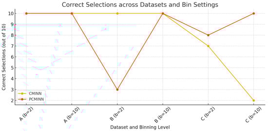
Figure 3.
Correct feature selections across all datasets and binning settings for both CMINN and PCMINN.
3.4. Case Study
To evaluate the practical applicability of PCMINN in a real-world scenario, we also compared it with CMINN using the Company Bankruptcy Prediction dataset, available on Kaggle [48]. This dataset contains financial indicators for Taiwanese companies, labeled as either bankrupt or non-bankrupt. It includes 6819 recordings (number of instances) and 96 financial indicators (features). The dataset was selected so as to involve many continuous-valued features (93 out of 96). Thus, beyond the class variable, only two of the remaining features are categorical, namely, Net Income Flag and Liability Assets Flag.
The primary goals of this evaluation are, first, to compare CMINN and PCMINN in terms of the runtime required to identify the optimal feature subsets and second, to compare the predictive performance of these subsets using standard classification models. Specifically, we set both methods to select subsets of the top 5, 10, 20 and 30 features. Following feature selection, we evaluated classification performance using three widely used classifiers: Logistic Regression, Decision Tree and Random Forest. Each model was trained and evaluated using 10-fold cross-validation and we report the mean accuracy and standard deviation across the folds.
Table 9 presents the execution time required by PCMINN and CMINN to identify the optimal feature subsets on the Bankruptcy Prediction dataset, across different subset sizes. As expected, both methods require more time as the number of selected features increases. However, PCMINN consistently outperforms CMINN in terms of computational efficiency. For example, when selecting 10 features, PCMINN completes in approximately 769 s, compared to 7076 s for CMINN—yielding nearly a 9.2× speedup. A similar pattern is observed across all evaluated subset sizes, where PCMINN consistently achieves faster execution—approximately 9.2 times faster than CMINN in all cases.
Table 9.
Execution time (in seconds) for PCMINN and CMINN on the Bankruptcy Prediction dataset across different numbers of selected features.
Table 10 presents the classification performance of PCMINN and CMINN across three classifiers and varying numbers of selected features. Overall, both methods demonstrate highly comparable results across all configurations, with differences in accuracy typically within 0.001–0.005. For Decision Trees, performance is nearly identical, with slight alternations between PCMINN and CMINN as the best-performing method at each feature subset size. In contrast, Logistic Regression consistently favors PCMINN, with PCMINN achieving higher accuracy in all subset sizes, by margins of approximately 0.005. For Random Forest, the two methods again perform similarly, with minor fluctuations. CMINN slightly outperforms PCMINN at 20 and 30 features, although the margins remain negligible and within standard deviation ranges.
Table 10.
Classification accuracy (mean ± std) using features selected by PCMINN and CMINN on Bankruptcy Prediction dataset. Accuracy is computed via 10-fold cross-validation.
These results indicate that PCMINN preserves the feature selection quality of the original CMINN method, with classification accuracy being statistically indistinguishable across methods and subset sizes. Combined with the significant runtime gains demonstrated earlier, this confirms that PCMINN offers a practical and scalable alternative to CMINN, without compromising selection performance.
In addition to the strong classification results, it is noteworthy that when selecting only five features, PCMINN and CMINN achieved excellent accuracy across all classifiers. The selected features were Return on Assets (ROA), Cash Flow per Share, Continuous Net Profit Growth Rate, Total Debt to Total Net Worth and Current Assets to Total Assets. These indicators are among the most informative and commonly used financial ratios in bankruptcy prediction and cover all key financial aspects of a company, including profitability, liquidity, growth, leverage and asset structure. ROA and Cash Flow per Share reflect profitability and liquidity, while the net profit growth rate provides a view of long-term performance. The debt to net worth ratio signals financial leverage and the current-to-total assets ratio reflects short-term solvency and operational efficiency. The inclusion of these features further supports the effectiveness of feature selection methods in selecting compact yet highly informative feature sets with real-world interpretability.
4. Discussion
This study introduced PCMINN, a GPU-accelerated variant of the CMINN algorithm, aiming to overcome the computational bottlenecks of high-dimensional feature selection using conditional mutual information. The results from the simulation study across three datasets (A, B and C) affirm that PCMINN preserves the selection accuracy of the original CMINN method while drastically improving runtime efficiency.
Across all datasets, PCMINN consistently identified the relevant features or achieved equivalent rankings as CMINN, particularly when the number of bins used for discretization was higher (e.g., ). The experiments demonstrated substantial speedups ranging from 5.3× to 8.3×, making PCMINN especially suitable for large-scale applications where computational cost is a limiting factor. It is important to emphasize that while the original CMINN implementation utilizes a KD-tree structure to accelerate nearest-neighbor searches on the CPU, PCMINN adopts a brute-force strategy on the GPU. Despite the higher theoretical complexity of brute-force search, the massive parallelism of modern GPUs compensates for this cost, resulting in significantly faster execution overall. In addition, we acknowledge that the original experiments were conducted on a modest system (GTX 1650 with 4 GB VRAM), as it was the only hardware available to us at the time. However, to validate the scalability of our approach, we have also executed the same experimental pipeline on Google Colab using an NVIDIA T4 GPU (15 GB VRAM). In this setup, execution times were approximately three times faster than these on the GTX 1650, confirming that PCMINN’s performance scales favorably with more capable GPU hardware.
In summary, while both methods converge to identical rankings under higher bin resolutions, the observed divergence in Dataset B for raises interesting questions regarding the stability of ranking under coarse discretization and highlights a potential trade-off between speed and precision in PCMINN under specific conditions. Given that PCMINN performs similarly (almost identical) to CMINN in feature selection and feature ranking in almost all other circumstances, this discrepancy is very noteworthy. Interestingly, when the exact same setup tested with a smaller sample size (), PCMINN produced results identical to CMINN, successfully identifying the correct subset in every run. This observation points to the possibility that the inconsistency seen at 10,000 and is more likely tied to the data characteristics, rather than to the algorithm itself.
A similar irregularity was observed in Dataset C, but in the opposite direction. This time, it was CMINN that failed to identify the optimal subset, especially under , where it selected the correct subset only 2 times, while PCMINN succeeded in all 10 runs. This reversal further reinforces the idea that deviations are more context-dependent than method-specific.
Initially, it was hypothesized that the occasional differences in feature selection between CMINN and PCMINN could be attributed to the different nearest-neighbor search methods employed, since CMINN leverages a KD-tree structure for k-nearest-neighbor search on CPU, whereas PCMINN uses a brute-force search entirely on GPU. To investigate this, we developed a brute-force version of CMINN (CMINN_brute) and repeated the experiments across all datasets. The results clearly showed that CMINN_brute yielded identical outputs to the original KD-tree-based CMINN, both in terms of feature selection accuracy and execution time. Furthermore, when comparing the two CPU variants on smaller datasets, it was found that KD-tree provides a time advantage only for sample sizes up to approximately , beyond which the performance of KD-tree and brute-force converges. These findings confirm that the choice of nearest-neighbor search algorithm alone cannot explain the observed discrepancies between PCMINN and CMINN.
Given that both CPU variants behave identically, the remaining differences must stem from factors inherent to the computational environments, namely, CPU versus GPU execution. While the core algorithm remains the same, PCMINN relies on GPU-accelerated libraries (cuML, CuPy) and parallelized computation, which introduce architectural and numerical differences. These include the use of single-precision floating-point arithmetic (float32) on GPU versus double-precision (float64) on CPU, as well as potential non-determinism in operation order due to concurrent execution across thousands of cores. Although these differences are typically negligible, they may become influential in edge cases where multiple features have nearly identical conditional mutual information scores. Such scenarios can lead to slight variations in tie-breaking behavior or neighborhood structure, ultimately affecting the ranking outcome. Importantly, these deviations are rare and in the vast majority of cases, PCMINN and CMINN produce identical results.
Together, these findings reinforce the conclusion that performance deviations between CMINN and PCMINN are not systematic, but rather context-dependent. They emerge from specific combinations of discretization, sample size and data structure. Despite these edge cases, PCMINN consistently replicates the behavior of CMINN in the vast majority of scenarios, offering significantly improved computational efficiency without sacrificing selection quality or classification performance.
This assumption is further reinforced by the fact that (as also demonstrated in the Section 3) when the same two iterations were randomly selected for both algorithms (to examine it in the same datasets), it was observed that they not only produced the same optimal subset, but the features were selected in the exact same order. In some cases, even the subsequent redundant selections involved the same irrelevant feature, highlighting the strong alignment between PCMINN and CMINN in practical execution.
Overall, this study confirms that parallelization through GPUs offers a practical and effective solution for scaling mutual information-based feature selection to high-dimensional data. The trade-off between speed and precision becomes negligible under appropriate parameter settings, especially when using finer binning or moderately sized datasets.
It should also be noted that no custom CUDA kernels were used in our implementation. Instead, this study serves as an initial exploration into GPU-based acceleration of CMI-based feature selection, relying exclusively on high-level libraries such as CuPy and cuML. While deeper performance optimization is possible through lower-level CUDA programming, our goal here was to demonstrate that significant speedups can be achieved even with minimal intervention and without diving into the complexities of kernel-level development.
Given that substantial performance improvements were achieved using only high-level GPU libraries, it is reasonable to expect that a low-level implementation, for instance, using custom CUDA kernels, would yield even greater speedups. This becomes especially promising when combined with more powerful computational infrastructures. Prior studies mentioned earlier have demonstrated the benefits of such optimizations and extending PCMINN in this direction could unlock its full potential for large-scale, real-time feature selection tasks. Therefore, a low-level GPU implementation combined with optimized hardware will constitute a promising direction for future research.
5. Conclusions
In this work, we presented PCMINN, a GPU-accelerated version of the Conditional Mutual Information Nearest-Neighbor (CMINN) algorithm, specifically designed to address the computational challenges associated with high-dimensional feature selection. By leveraging parallel processing capabilities of modern GPUs through libraries such as CuPy and cuML, PCMINN achieves substantial reductions in execution time, while preserving the accuracy and the reliability of the original CMINN algorithm. We also provide a package that includes two implementations for Python to support its integration in future research workflows: a sequential one of CMINN and a parallel one for GPUs of PCMINN.
Extensive simulations on synthetic datasets demonstrated that PCMINN performs comparably to CMINN in terms of identifying relevant features, even in the presence of nonlinear dependencies and redundant variables. The results also showed that PCMINN consistently offers a speedup ranging from five to eight times over its CPU-based counterpart, even though in this initial implementation it relies exclusively on high-level libraries such as CuPy and cuML. This makes it a promising tool for large-scale, real-world applications where computational efficiency is critical.
Future improvements may focus on low-level GPU implementations using custom CUDA kernels, which are expected to further enhance performance, especially when combined with more powerful computing systems.
Author Contributions
Conceptualization, N.P. and A.T.; methodology, N.P., G.M. and A.T.; software, N.P.; validation, N.P., G.M. and A.T.; formal analysis, N.P.; investigation, N.P.; resources, N.P. and G.M.; data curation, N.P.; writing—original draft preparation, N.P. and G.M.; writing—review and editing, N.P., G.M., A.T., S.A. and V.V.; visualization, N.P., A.T. and V.V.; supervision, A.T., S.A. and V.V.; project administration, A.T., S.A. and V.V. All authors have read and agreed to the published version of the manuscript.
Funding
This research received no external funding.
Data Availability Statement
The code used in this study is available at https://github.com/pcminn-dev/cminn-pcminn-feature-selection, accessed on 1 May 2025.
Conflicts of Interest
The authors declare no conflicts of interest.
References
- Laney, D. 3D Data Management: Controlling Data Volume, Velocity, and Variety; META Group: Stamford, CT, USA, 2001. [Google Scholar]
- Chen, M.; Mao, S.; Liu, Y. Big Data: A Survey. Mob. Netw. Appl. 2014, 19, 171–209. [Google Scholar] [CrossRef]
- Morgenstern, J.; Rosella, L.; Costa, A.; de Souza, R.; Anderson, L. Perspective: Big Data and Machine Learning Could Help Advance Nutritional Epidemiology. Adv. Nutr. 2021, 12, 621–631. [Google Scholar] [CrossRef] [PubMed]
- Krizhevsky, A.; Sutskever, I.; Hinton, G.E. ImageNet Classification with Deep Convolutional Neural Networks. In Proceedings of the Advances in Neural Information Processing Systems (NeurIPS), Lake Tahoe, NV, USA, 3–6 December 2012. [Google Scholar]
- Guyon, I.; Elisseeff, A. An Introduction to Variable and Feature Selection. J. Mach. Learn. Res. 2003, 3, 1157–1182. [Google Scholar]
- Stamper, J.; Pardos, Z. The 2010 KDD Cup Competition Dataset: Engaging the Machine Learning Community in Predictive Learning Analytics. J. Learn. Anal. 2016, 3, 312–316. [Google Scholar] [CrossRef]
- Zhang, D.; Hao, X.; Wang, D.; Qin, C.; Zhao, B.; Liang, L.; Liu, W. An efficient lightweight convolutional neural network for industrial surface defect detection. Artif. Intell. Rev. 2023, 56, 10651–10677. [Google Scholar] [CrossRef]
- Zhang, D.; Wang, Y.; Meng, L.; Yan, J.; Qin, C. Adaptive critic design for safety-optimal FTC of unknown nonlinear systems with asymmetric constrained-input. ISA Trans. 2024, 155, 309–318. [Google Scholar] [CrossRef]
- Yu, L.; Liu, H. Efficient Feature Selection via Analysis of Relevance and Redundancy. J. Mach. Learn. Res. 2004, 5, 1205–1224. [Google Scholar]
- Verleysen, M.; François, D. The Curse of Dimensionality in Data Mining and Time Series Prediction. In Computational Intelligence and Bioinspired Systems, Proceedings of the 8thInternational Work-Conference on Artificial Neural Networks, IWANN 2005, Vilanova i la Geltrú, Spain, 8–10 June 2005; Springer: Berlin/Heidelberg, Germany, 2005; Volume 3512, pp. 758–770. [Google Scholar] [CrossRef]
- Ye, J.; Liu, H. Challenges of Feature Selection for Big Data Analytics. IEEE Intell. Syst. 2017, 32, 9–15. [Google Scholar] [CrossRef]
- McCrory, M.N.F.; Thomas, S.A. Cluster Metric Sensitivity to Irrelevant Features. In Computational Problems in Science and Engineering II; Mastorakis, N.E., Rudas, I.J., Shmaliy, Y.S., Eds.; Springer Nature: Cham, Switzerland, 2025; pp. 85–95. [Google Scholar] [CrossRef]
- Mittal, S.; Shuja, M.; Zaman, M. A Review of Data Mining Literature. IJCSIS 2016, 14, 437–442. [Google Scholar]
- Joel, M.R.; Rajakumari, K.; Priya, S.A.; Navaneethakrishnan, M. Big data classification using SpinalNet-Fuzzy-ResNeXt based on spark architecture with data mining approach. Data Knowl. Eng. 2024, 154, 102364. [Google Scholar] [CrossRef]
- Manley, K.; Nyelele, C.; Egoh, B.N. A review of machine learning and big data applications in addressing ecosystem service research gaps. Ecosyst. Serv. 2022, 57, 101478. [Google Scholar] [CrossRef]
- Thomas, S.A.; Race, A.M.; Steven, R.T.; Gilmore, I.S.; Bunch, J. Dimensionality reduction of mass spectrometry imaging data using autoencoders. In Proceedings of the 2016 IEEE Symposium Series on Computational Intelligence (SSCI), Athens, Greece, 6–9 December 2016; pp. 1–7. [Google Scholar] [CrossRef]
- Yue, X.; Liao, Y.; Peng, H.; Kang, L.; Zeng, Y. A high-dimensional feature selection algorithm via fast dimensionality reduction and multi-objective differential evolution. Swarm Evol. Comput. 2025, 94, 101899. [Google Scholar] [CrossRef]
- Süpürtülü, M.; Hatipoğlu, A.; Yılmaz, E. An Analytical Benchmark of Feature Selection Techniques for Industrial Fault Classification Leveraging Time-Domain Features. Appl. Sci. 2025, 15, 1457. [Google Scholar] [CrossRef]
- Ruano-Ordás, D. Machine Learning-Based Feature Extraction and Selection. Appl. Sci. 2024, 14, 6567. [Google Scholar] [CrossRef]
- Linja, J.; Hämäläinen, J.; Nieminen, P.; Kärkkäinen, T. Feature selection for distance-based regression: An umbrella review and a one-shot wrapper. Neurocomputing 2023, 518, 344–359. [Google Scholar] [CrossRef]
- Xu, W.; Tian, Z. Feature selection and information fusion based on preference ranking organization method in interval-valued multi-source decision-making information systems. Inf. Sci. 2025, 700, 121860. [Google Scholar] [CrossRef]
- Verma, A.; Yadav, A.K. FusionNet: Dual input feature fusion network with ensemble based filter feature selection for enhanced brain tumor classification. Brain Res. 2025, 1852, 149507. [Google Scholar] [CrossRef]
- Solorio-Fernández, S.; Carrasco-Ochoa, J.A.; Martínez-Trinidad, J.F. Filter unsupervised spectral feature selection method for mixed data based on a new feature correlation measure. Neurocomputing 2024, 571, 127111. [Google Scholar] [CrossRef]
- Mohino-Herranz, I.; Gil-Pita, R.; García-Gómez, J.; Rosa-Zurera, M.; Seoane, F. A Wrapper Feature Selection Algorithm: An Emotional Assessment Using Physiological Recordings from Wearable Sensors. Sensors 2020, 20, 309. [Google Scholar] [CrossRef]
- Papaioannou, N.; Tsimpiris, A.; Talagozis, C.; Fragidis, L.; Angeioplastis, A.; Tsakiridis, S.; Varsamis, D. Parallel Feature Subset Selection Wrappers Using k-means Classifier. Wseas Trans. Inf. Sci. Appl. 2023, 20, 76–86. [Google Scholar] [CrossRef]
- Li, J.; Zhang, H.; Zhao, J.; Guo, X.; Rihan, W.; Deng, G. Embedded Feature Selection and Machine Learning Methods for Flash Flood Susceptibility-Mapping in the Mainstream Songhua River Basin, China. Remote Sens. 2022, 14, 5523. [Google Scholar] [CrossRef]
- Carrasco, M.; Ivorra, B.; López, J.; Ramos, A.M. Embedded feature selection for robust probability learning machines. Pattern Recognit. 2025, 159, 111157. [Google Scholar] [CrossRef]
- Bai, Y.; Dong, Z.; Liu, L. Hybrid feature selection-based machine learning methods for thermal preference prediction in diverse seasons and building environments. Build. Environ. 2025, 269, 112450. [Google Scholar] [CrossRef]
- Abdo, A.; Mostafa, R.; Abdel-Hamid, L. An Optimized Hybrid Approach for Feature Selection Based on Chi-Square and Particle Swarm Optimization Algorithms. Data 2024, 9, 20. [Google Scholar] [CrossRef]
- Sun, L.; Xu, F.; Ding, W.; Xu, J. AFIFC: Adaptive fuzzy neighborhood mutual information-based feature selection via label correlation. Pattern Recognit. 2025, 164, 111577. [Google Scholar] [CrossRef]
- Huang, L.; Zhou, X.; Shi, L.; Gong, L. Time Series Feature Selection Method Based on Mutual Information. Appl. Sci. 2024, 14, 1960. [Google Scholar] [CrossRef]
- Morán-Fernández, L.; Blanco-Mallo, E.; Sechidis, K.; Bolón-Canedo, V. Breaking boundaries: Low-precision conditional mutual information for efficient feature selection. Pattern Recognit. 2025, 162, 111375. [Google Scholar] [CrossRef]
- Ding, C.; Peng, H. Minimum Redundancy Feature Selection from Microarray Gene Expression Data. J. Bioinform. Comput. Biol. 2005, 3, 185–205. [Google Scholar] [CrossRef]
- Hoque, N.; Bhattacharyya, D.; Kalita, J. MIFS-ND: A mutual information-based feature selection method. Expert Syst. Appl. 2014, 41, 6371–6385. [Google Scholar] [CrossRef]
- Papana, A.; Kugiumtzis, D. Evaluation of mutual information estimators for time series. Int. J. Bifurc. Chaos 2009, 19, 4197–4215. [Google Scholar] [CrossRef]
- Tsimpiris, A.; Vlachos, I.; Kugiumtzis, D. Nearest neighbor estimate of conditional mutual information in feature selection. Expert Syst. Appl. 2012, 39, 12697–12708. [Google Scholar] [CrossRef]
- Kraskov, A.; Stögbauer, H.; Grassberger, P. Estimating mutual information. Phys. Rev. E 2004, 69, 066138. [Google Scholar] [CrossRef] [PubMed]
- Myllis, G.; Tsimpiris, A.; Aggelopoulos, S.; Vrana, V. High-Performance Computing and Parallel Algorithms for Urban Water Demand Forecasting. Algorithms 2025, 18, 182. [Google Scholar] [CrossRef]
- González-Domínguez, J.; Expósito, R.R.; Bolón-Canedo, V. CUDA-JMI: Acceleration of feature selection on heterogeneous systems. Future Gener. Comput. Syst. 2020, 102, 426–436. [Google Scholar] [CrossRef]
- Ramírez-Gallego, S.; Lastra, I.; Martinez, D.; Bolón-Canedo, V.; Benítez, J.; Herrera, F.; Alonso-Betanzos, A. Fast-mRMR: Fast Minimum Redundancy Maximum Relevance Algorithm for High-Dimensional Big Data: FAST-mRMR ALGORITHM FOR BIG DATA. Int. J. Intell. Syst. 2016, 32, 134–152. [Google Scholar] [CrossRef]
- Beceiro, B.; González-Domínguez, J.; Morán-Fernández, L.; Bolón-Canedo, V.; Touriño, J. CUDA acceleration of MI-based feature selection methods. J. Parallel Distrib. Comput. 2024, 190, 104901. [Google Scholar] [CrossRef]
- Shannon, C.E. A mathematical theory of communication. Bell Syst. Tech. J. 1948, 27, 379–423. [Google Scholar] [CrossRef]
- Paninski, L. Estimation of Entropy and Mutual Information. Neural Comput. 2003, 15, 1191–1253. [Google Scholar] [CrossRef]
- Qian, X. Topology optimization in B-spline space. Comput. Methods Appl. Mech. Eng. 2013, 265, 15–35. [Google Scholar] [CrossRef]
- Weglarczyk, S. Kernel density estimation and its application. ITM Web Conf. 2018, 23, 00037. [Google Scholar] [CrossRef]
- Hu, Q.; Zhang, L.; Zhang, D.; Wei, P.; An, S.; Pedrycz, W. Measuring relevance between discrete and continuous features based on neighborhood mutual information. Expert Syst. Appl. 2011, 38, 10737–10750. [Google Scholar] [CrossRef]
- Vlachos, I.; Kugiumtzis, D. Nonuniform state-space reconstruction and coupling detection. Phys. Rev. E 2010, 82, 016207. [Google Scholar] [CrossRef] [PubMed]
- Soriano, F. Company Bankruptcy Prediction. 2020. Available online: https://www.kaggle.com/datasets/fedesoriano/company-bankruptcy-prediction (accessed on 9 May 2025).
Disclaimer/Publisher’s Note: The statements, opinions and data contained in all publications are solely those of the individual author(s) and contributor(s) and not of MDPI and/or the editor(s). MDPI and/or the editor(s) disclaim responsibility for any injury to people or property resulting from any ideas, methods, instructions or products referred to in the content. |
© 2025 by the authors. Licensee MDPI, Basel, Switzerland. This article is an open access article distributed under the terms and conditions of the Creative Commons Attribution (CC BY) license (https://creativecommons.org/licenses/by/4.0/).