Abstract
Anomaly-based attack detection methods depend on some form of machine learning to detect data falsification attacks in smart living cyber–physical systems. However, there is a lack of studies that consider the presence of attacks during the training phase and their effect on detection and false alarm performance. To improve the robustness of time series learning for anomaly detection, we propose a framework by modifying design choices such as regression error type and loss function type while learning the thresholds for an anomaly detection framework during the training phase. Specifically, we offer theoretical proofs on the relationship between poisoning attack strengths and how that informs the choice of loss functions used to learn the detection thresholds. This, in turn, leads to explainability of why and when our framework mitigates data poisoning and the trade-offs associated with such design changes. The theoretical results are backed by experimental results that prove attack mitigation performance with NIST-specified metrics for CPS, using real data collected from a smart metering infrastructure as a proof of concept. Thus, the contribution is a framework that guarantees security of ML and ML for security simultaneously.
1. Introduction
Data falsification attacks from sensors have been widely studied in cyber–physical system (CPS) domains. The objective of data falsification attacks is to disrupt the operational accuracy and functioning of a CPS application. To detect such attacks, anomaly detection approaches, which involve some form of machine learning (ML), have been developed. For example, in CPS anomaly detection, a series of works proposed in [1,2,3] involve learning a low dimensional representation of the benign profile of sensing data from a large distributed network of CPS sensors. This is followed by learning a detection threshold of the benign profile from the low dimensional representation. However, all these works assume that the training data are attack- and error-free.
In contrast, the discipline of adversarial ML deals with attacks that are analogous to data falsification attacks, but designed specifically to exploit inherent weaknesses in the ML/AI principles [4,5,6] and may happen during training. Naturally, therefore, learning-based anomaly detection frameworks designed to detect data falsification attacks are themselves vulnerable to adversarial ML attacks. Therefore, there is a need to design robust learning-based anomaly detection frameworks that are gracefully immune to adversarial ML attacks, while still being able to detect those attacks that the anomaly detection approach was originally designed to identify.
Proof-of-Concept Application: To show experimental validity of our work, we use smart metering infrastructure (SMI) as a smart living CPS sensing proof-of-concept application. We consider a neighborhood of households each installed with a smart energy meters that sense power consumption data periodically. We select a state-of-the-art learning-based anomaly detector (See Section 3 for formal details) that was developed to identify electricity theft and other attacks in SMI [1] during the testing phase by accurately learning the thresholds of a latent space that specified benign behavior of a network of smart meters from a neighborhood. The work in [1] proved that any data falsification attack from one or more smart meters during test phase (that in the real world can result from cyber attack/physical tampering of meters) violates the learned thresholds of benign behavior from training data containing smart meter power consumption data.
However, for any kind of machine learning to be successful, the training and test data should ideally come from the same distribution. Therefore, learning the profile of benign data during training must be performed on data collected from the actual SMI deployment. Naturally, even though the adversary does not know the exact detection model, they know that falsifying data during training will degrade the learning performance of the anomaly-based attack detector by preventing accurate profiling of benign behavior. Infact, an audit study [7] conducted across several countries revealed the presence of organized manipulation of smart meters which biases any data collected.
Scope: Within adversarial ML, attacks are broadly categorized as evasion and poisoning. Data poisoning attacks falsify data during the training phase, thereby preventing accurate learning and negatively affecting the performance of the ML-based framework during the test phase. In this paper, we focus on the mitigating impact of ’data poisoning attacks’ [8] on anomaly-based attack detection methods that use machine learning principles. Furthermore, adversarial ML attacks specify varying possible levels of knowledge an adversary could possess: (1) white-box, (2) black-box, (3) gray-box. In a white-box, the adversary is assumed to have exact knowledge of the ML technique and direct access to all training/test data points, representing the worst-case scenario. In the black-box approach, the attacker has no knowledge of the model and partial access to the data. The gray-box approach falls in between, where the adversary has some knowledge of the model and partial access to the data points. Although white-box strategies can have serious consequences, the likelihood of such attacks is lower compared to black-box attacks that are much easier to launch and hence more likely (especially in the context of our chosen proof-of-concept application smart metering infrastructure). Hence, in this paper, we focus on the black-box approach to data poisoning given its high likelihood.
We implement data falsification attacks of varying intensities over varying possible subsets compromised by smart meters (termed as Random Smart Meter Level poisoning attack (RSL)) during the training phase to emulate various potential intents of an attacker. This biases the learned low-dimensional latent representation of the feature space and hence its detection thresholds. We apply our modified threshold learning approach and then evaluate the impact of undetected attacks with and without the presence of data poisoning and compare with the approach proposed in [1]. We observe a significant degradation in the anomaly detection model’s performance proposed in [1] while proving that proposed advancements on detection threshold learning via resilient and adaptive M-estimation theory mitigates the impact of undetected attacks in the test set caused by data poisoning attacks launched during training.
Contributions: (1) We propose a novel robust learning framework for learning anomaly detection thresholds by integrating weighted regression and the theory of M-estimators.
(2) We demonstrate the relationship between the data poisoning attack strength and how it impacts the loss function choice, and a very counter-intuitive false alarm trade-off that accounts for the lower base rate probability of experiencing a data poisoning attack.
(3) We develop formal, explainable theoretical proofs that show which loss function offers mitigation, and why, under different intensities of data poisoning attacks.
(4) We compare improvements of the proposed resilient ML-based anomaly detection over prior works using two unconventional metrics for more practical security evaluation: (a) impact of undetected attacks; (b) expected time between two false alarms.
Benefits: We take a unique approach of breaking down the anomaly detection framework into its key facets (anomaly detection metric latent space, effect of regression type choice, effect of loss function choice, effect of base rate fallacy). Furthermore, this is in contrast to other works which just randomly try different loss functions and find the best one empirically. Additionally, we show which data and attack characteristics should be used and how to optimally derive the best loss function (i.e., estimator of parameter) that should be used for learning in an application agnostic manner by focusing on distribution characteristics in the regression errors over the latent anomaly detection metric being used for attack/anomaly detection. We provide explainability of why the proposed mitigation framework really works with the associated trade-offs, and failure points via our chosen metrics of evaluation, such as the impact of undetected attacks.
A preliminary version of this work appeared in [9]. However, the earlier paper did not (i) prove why this mitigation occurs, (ii) explain the design choices made for anomaly detection learning, and why and when they are appropriate against data poisoning attacks, and (iii) have theoretical results that verify the correctness of the experimental outcomes. In this paper, we address (i), (ii), and (iii) to provide a proper scientific foundation for the preliminary work.
2. Related Work
There is one work on adversarial machine learning that discusses smart grids in the context of differential privacy [10]. For poisoning attacks and defenses in a general regression setting, Ref. [11] proposes an adversarial poisoning technique that adds extra points to an existing dataset to bias the prediction in a classical linear regression problem. This approach works in an open setting but is not applicable in a CPS setting, where all smart meters must be physically registered with a utility. Some works [12] have proposed game-theoretic defenses for theoretical regression problems involving a rational adversary, which are valid under white-box attack assumptions, where the adversary both knows the detection model and has access to all training data points. In [11], the attack in a regression setting involved adding extra points to the training set, and the defense limited the inclusion of these extra points in the learning process. However, in our case, time is an invariant design feature, making the addition of extra points for poisoning infeasible. There have been significant theoretical advances in evaluating the vulnerabilities of ML models against adversarial attacks, particularly in computer vision and image processing algorithms [4,13]. Additionally, practical works on adversarial attacks targeting spam email detection [5], as well as various theoretical studies on attacks and defenses [11], also exist. Most existing work in smart living CPS focuses on strategies that disrupt operations, but does not explain the mitigation of data poisoning attacks that target the machine learning aspect of anomaly-based data integrity attack detectors.
3. Background and Preliminaries
The SMI consists of smart meters deployed in houses that periodically collect power consumption data. At any hour t, the power consumption reported by the i-th smart meter in house i is denoted as . We now provide the details of the anomaly detection process.
3.1. Anomaly Detection Problem Specification
The model being poisoned is a time series anomaly detection method proposed in a series of previous works [1,3,14,15]. We chose this technique due to the following reasons: (1) it represents the most recent theoretical work in micro-grid-level time series anomaly detection, capable of detecting very low data falsification margins while maintaining a low false alarm rate; (2) the method has been shown to generalize to other CPS/IoT domains such as Phasor Measurement Units [15], Smart Transportation Systems [3], and Smart Water Usage Monitoring [14]; (3) it adheres to the latest National Institute of Standards and Technology (NIST)-specified metrics [2], such as the impact of undetected attacks and expected time between false alarms; (4) while many anomaly detection methods in industrial CPS rely on pairwise comparison of positive covariance structures [16] for invariant design, such calculations are expensive for large community-scale smart living CPS (like SMI). The method in [1] proposes a lightweight equivalent. Additionally, the chosen framework’s metrics show unique deviation signatures under different data integrity attack types, which assist in reconstructing the attack type, strategy, and severity.
The goal of the anomaly detection framework in the test set is to detect orchestrated data falsification attacks in a smart metering infrastructure. Poisoning attacks, on the other hand, aim to alter the training data, degrading the model’s performance in the test set in two ways: (1) integrity violation, which aims to increase missed detections, and (2) availability violation, which aims to increase the false alarm rate.
In this paper, we focus solely on integrity violations caused by poisoning attacks. While our poisoning attack targets a specific technique proposed in [1], it generalizes to other time series anomaly detection methods that use regression-based learning to determine anomaly detection thresholds. This generality arises from the shared design similarities among time series anomaly detection approaches.
To provide a generic contribution while demonstrating the practical effectiveness of a specific framework and application, we describe the anomaly detection technique [1] through the following key aspects: (1) anomaly detection metric, (2) residuals of a time series, (3) learning of thresholds from residuals, and (4) anomaly detection criterion.
3.2. Time Series Anomaly Detection Method
The anomaly detection method converts the raw data into a latent space called that is a low-dimensional time series representation. We provide the steps below:
Anomaly detection Metric: The anomaly detection metric is a time series of the harmonic-to-arithmetic mean ratio from multiple smart meters (proposed in [1,15]). To achieve invariance in the time series of the metric under benign conditions, the ratio is calculated over strategic spatial and temporal granularity, designed to maximize positive covariance among individual meters in the micro-grid. Mathematically, the invariant metric is as follows:
where and are the harmonic and arithmetic means of power consumption from 200 smart meters at time slot t, after applying a Box-Cox transformation. The temporal granularity is indexed by the T-th time window, with each time window consisting of a length of W time slots.
In the case of SMI, previous work determined that h, and the granularity included the entire solar village of 200 houses due to its small size. Hence, for a typical year, the range of . This method operates in a decentralized manner for each spatial cluster. In this paper, we focus on a single spatial cluster, specifically a small solar village forming a micro-grid of 200 houses.
Safe Margins: Safe margins quantify the expected upper and lower bounds of the anomaly detection metric at any time window T. The expected value of the ratio metric at the T-th time window is denoted as . is the cumulative weighted time average of ratios observed across the T-th window over multiple years (non-parametric statistic). In contrast, denotes the standard deviation of the probability distribution of samples in the training set (parametric statistic). The upper and lower safe margins are neighborhoods around the expected value , controlled by a scalar factor of the standard deviation () of the distribution of the ratio metric. Mathematically, this is
where is the upper safe margin and the is the lower safe margin. The conceptual details of why this is helpful can be found in [1].
Latent Space Metric: The concept of residual latent space metric is important for balancing missed detections and false alarms in time series learning-based anomaly detection. Residuals represent the difference between the sample and the safe margins. The residual at any time window, , equals 0 if is within the upper and lower safe margins, and is non-zero when falls outside these margins. A larger than (outside the upper safe margin) results in a positive , while smaller than (outside the lower safe margin) results in a negative . Mathematically, this is represented as follows:
The are known as stateless residuals [16]. The corresponding stateful residuals are obtained from the stateless residuals by calculating the cumulative sum of over a sliding window of length F. At any T, the stateful residual is given by
Thus, the vector of per year has 365 entries, which can be zero, positive, or negative.
Threshold Learning from Latent Space: Using the positive values (denoted by ) as training data points, the best upper threshold () is found. Similarly, all negative values are used as training data points for determining the best lower threshold (). Setting a threshold from the set of discrete and points is similar to fitting a straight line to the set of points; thus, the threshold learning problem is treated as a regression problem. Since the threshold is time-invariant, the regression reduces to finding the bias term, which is the unknown model parameter. The search spaces for the upper and lower thresholds are denoted by and , respectively. We now introduce some terminology related to regression analysis for completeness and clarity:
Regression Error: In regression problems, the error is the difference between a candidate model parameter (or threshold) and a training data point. For each candidate model parameter, an error value is calculated for each training data point. In linear regression, positive and negative errors are treated equally. This is denoted as .
Loss Function: The loss function represents the regression error, indicating the fit of the candidate model parameters and . For example, linear regression uses the square of the regression error ( norm). For each candidate model parameter and training data point, there is one corresponding loss value.
Empirical Risk Function: It is an equation that maps the goodness of a candidate parameter across all training data points (observations). Typically, it is the average of the loss function values across all training data points. In linear regression, the empirical risk is typically the mean of squared errors. Since regression involves finding the function that best approximates the data, the candidate model parameter with the minimum empirical risk is the optimal solution. Hence, this type of regression is known as least squares regression.
A series of prior works in smart living CPS [1] argues that the norm (absolute errors), rather than the norm (squared regression error), should be used as the loss function to improve robustness against unpredictable human behaviors that affect the benign pattern in the latent space . Algorithm 1 summarizes the basic framework for learning thresholds as proposed in [1]. In Algorithm 1, the regression error is . Notice that, unlike in linear regression, the regression errors are assigned unequal weights, and the weighted regression errors are stored separately in and .
| Algorithm 1: Calculate |
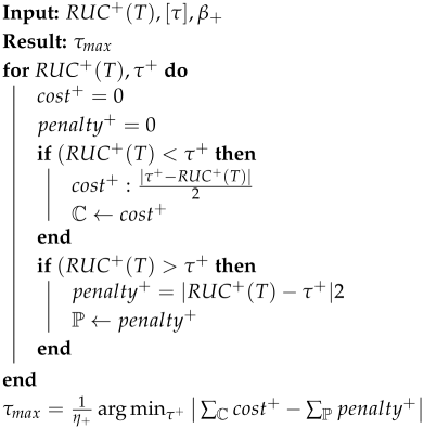 |
Detection Criterion: The is the invariant in the test set. If it is violates the upper and lower thresholds, it indicates an attack.
Using this approach, prior work [1] demonstrated that small-margin additive attacks increase , violating the upper threshold . For other attack types, such as deductive/camouflage attacks, decreases, violating the lower threshold .
4. Threat Model
The main goal of poisoning attacks is to reduce the learning accuracy of the detector during the training phase, allowing attacks to go undetected in the test set. This occurs when training phase attacks result in the widening of the true thresholds (i.e., the upper threshold increases and the lower threshold decreases). Additionally, the adversarial goal requires two threat models: one for the training set and one for the test set.
4.1. Training Phase Threat Model
The adversary injects false data into the training phase through a subset of compromised smart meters. As we show in Section 4.2, this biases the anomaly detection metric used to profile benign behavior. Utilities may not always face attacks from optimal adversaries. An attacker can poison the training process by introducing false data directly through smart meters (or other physical sensors) by compromising a subset of smart meters (referred to as attack scale) and injecting a specific amount of false data per smart meter (referred to as attack strength). In reality, both attack scale and strength can take on any value. To model this, we vary the attack scale and strength to create multiple simulated attack datasets, leading to a more comprehensive evaluation of potential threats.
Training Attack Strength, denoted by , refers to the average margin of false data injected per meter during training. The is used as a variable to assess the sensitivity of performance degradation in the anomaly detector.
Training Attack Scale, denoted by , refers to the fraction of meters used by an adversary to launch meter-level training data poisoning. is used as a variable to assess the sensitivity of the detector’s performance degradation.
Training Attack Type: This refers to how the data are falsified from their original value, . Several attack types relevant to SMI have been reported in [1] (e.g., additive, camouflage, conflict). In the context of poisoning aimed at violating the detector’s integrity, we found that a deductive attack type launched during the training phase is sufficient to achieve this. Details are provided in Section 4.2.
Deductive attacks reduce the original data, represented as , where , and the expected value of converges to the strategic Training Attack Strength . Furthermore, deductive data falsification attacks are easy to launch, particularly on smart meters, and a large fraction of smart meters are plagued by deductive attacks [7], leading to electricity theft, and making it a highly relevant problem when training anomaly-based attack detectors in SMI.
4.2. Investigating Impact of Data Poisoning on Latent Spaces in Anomaly Detection
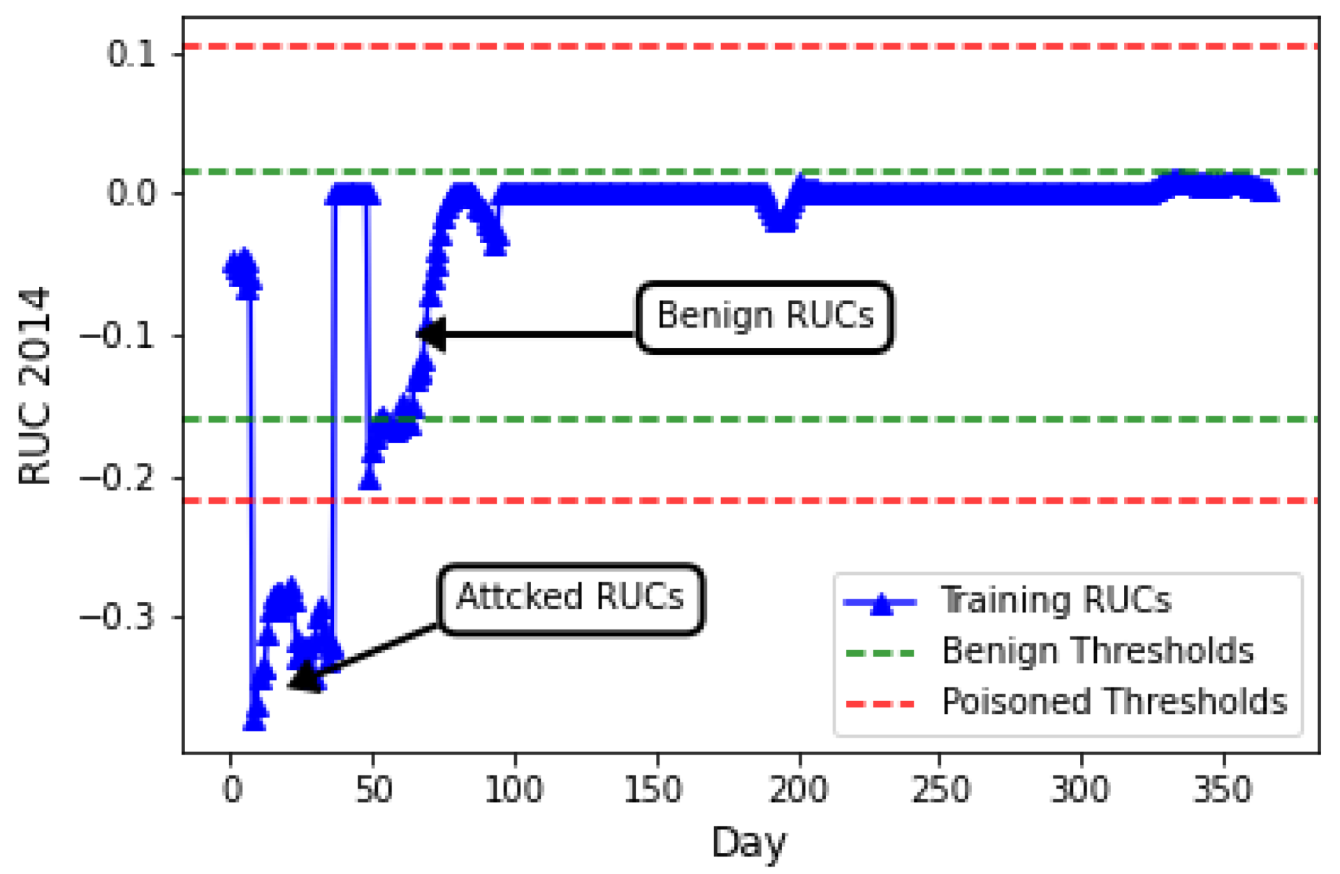
Random poisoning at the smart meter level gives adversaries a distinct advantage. It is more practical because it can be launched at any time, requiring only access to a set of CPS sensing endpoints (e.g., smart meters) and no other knowledge. In machine learning, the training and test sets should ideally come from the same distribution, which means training on actual smart living CPS system data is necessary. However, the attacks the utility aims to detect during testing may already be present in the training set. In such cases, we need to make the learning process more robust in Algorithm 1 when or inputs are perturbed. This is exactly what happens if there is a deductive attack from varying percentages of smart meters in a micro-grid. Figure 1 illustrates the impact of a basic deductive attack with and over a 1-month period during the training of a model using live smart meter deployment on . As the ratio and decrease, more negative RUCs appear in , influencing the learning of (See). This results in a lower being triggered by the negative RUCs.

Figure 1.
Latent space : benign vs. poisoned.
Generally, for most anomaly detection metrics (including ), higher and lead to greater deviations in the metric, indicating stronger poisoning impacts. However, when is excessively high, evident changes in the space may occur. Additionally, benign changes (refer to 50–100) highlight the necessity of threshold learning. Interestingly, the learned upper threshold also increases following a poisoning attack. This unexpected outcome arises due to the design of safe margins and , which aimed to reduce false alarms in the initial approach. Thus, robust learning for both thresholds is essential. Additionally, clustering-based methods to identify potential points are not unified, as the number of clusters formed a priori is unknown and depends on the specific values of and , with various combinations potentially used by an adversary. From the above analysis, we can infer that threshold learning is compromised in both directions. This finding is particularly noteworthy, as a single type of poisoning attack (i.e., deductive) during training can impact both the upper and lower thresholds, as illustrated in Figure 1. This manipulation enables the evasion of detection during testing.
4.3. Test Phase Threat Model
The test set threat model mirrors the smart meter-level perturbation, as the goal is to prevent the utility from detecting data falsification from smart meters. Therefore, we will not elaborate on this section but will use different notations, introducing the terms for attack strength and for attack scale, both used for evasion in the test set. This holds true whether residuals or raw meter data were perturbed during poisoning.
5. Resilient Learning Under Poisoning Attacks
We need to design a threshold learning method that mitigates the bias induced in the threshold estimate. In typical linear regression, the empirical loss function is , where the i-th training data point, denoted by (the RUC in our case), is formally called the residual. represents the difference between the data point and a given candidate estimate, expressed as , formally called the regression error. The poisoning attack causes the magnitude of to change, which in turn perturbs , affecting the threshold learning through regression. To achieve the above, we first provide theoretical insight into robust learning under poisoning attacks, including M-estimation. Second, we provide theoretical proof for the choice of M-estimators by demonstrating their theoretical relationship with poisoning attack strength. Third, we propose a robust algorithm for learning thresholds from the latent space.
5.1. Theoretical Intuition on Robust Learning Estimator
In the subsequent analysis, we explain how to determine a suitable loss function tailored to the specific characteristics of the attack and the rationale behind it. During the training phase, attackers can inject random attacks with different values of and . This manifests as varying degrees of perturbation in the latent space. Let the varying degree of perturbations be denoted as . These different poisoning attacks will lead to changes in regression errors (denoted as ) for each point in the latent space. The perturbation in the latent space depends on the product of the margin of false data (attack strength) and attack scale , resulting in a specific perturbation value of in the latent space, as shown in Section 4.2. In general, increasing and leads to a larger . The distribution of samples, contaminated by a margin , is defined as follows:
where refers to a normal (or ideal) distribution, typically representing the assumed parametric model of , and G represents an arbitrary symmetric distribution for contaminated that captures deviations from . The parameter and/or significantly influences the perturbed values, which in turn result in perturbed regression errors , introducing variations and deviations from the assumed parametric model (i.e., the normal distribution in regression). This influence is reflected in the distribution G, which captures the contaminated . As increases, the contamination in becomes more pronounced. On the other hand, the complementary value has a notably smaller influence. This component accounts for the portion of perturbed that still follows the normal distribution , belonging to the portion of training data that remains unpoisoned. Although present, these have a relatively minor impact compared to those captured by the distribution G.
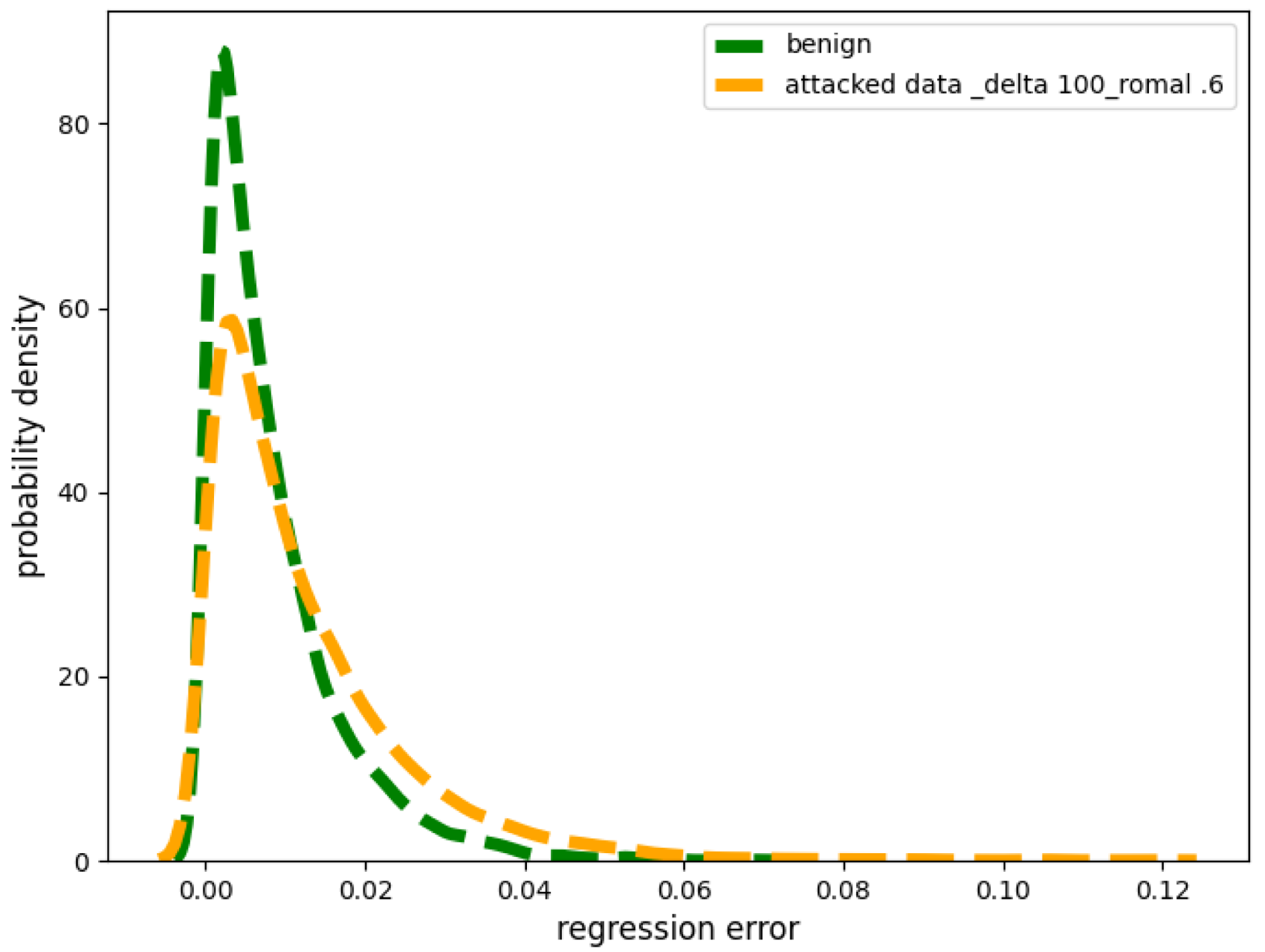
Small Strength Poisoning Attacks: Figure 2 depicts the two probability distributions originating from the two distinct sets (poisoned and non-poisoned) of regression errors. The yellow line in Figure 2 corresponds to the perturbed values arising from poisoned values represented by G. Specifically, the poisoning attack we implemented had a very small and we kept the . After performing a Kolmogorov–Smirnov test [17,18], we found that the contaminated distribution G most closely fits a double exponential distribution. However, note that the above is only true when is relatively small, given the same value of .

Figure 2.
Benign versus contaminated distribution of regression errors under low of 100 W from smart meters.
In contrast, the green line in Figure 2 represents the distribution of benign regression errors originating from the benign values, denoted as . The Kolmogorov–Smirnov test revealed that most closely fits the Gaussian distribution.
This distribution P is a composite distribution where the central region is approximated by a mixture of normal distributions (), while the tail section resembles a double exponential distribution (G).
is the scale parameter of the input set and is a constant, where is a separating point dividing the compound distribution such that points smaller than come from the unperturbed true Gaussian distribution , and points greater than follow a double exponential distribution. As mentioned in [19], in the most general case, guessing the least favorable distribution allows for hypothesis testing on compound distributions, as in our case. Hence, we can rewrite Equation (7), as a least favorable distribution, by the following:
where and correspond to the location and scale parameters of the least favorable distribution (i.e., the regression errors ), and represents the pdf of a normal distribution. The second part represents the pdf of a double exponential distribution. Without loss of generality, Equation (8) is the density function for the least favorable distribution.
Following the theory of least favorable distributions, the pdf is not expressed via the raw input , but rather a standardized input. An estimator is known as “minimax” when it performs best in the worst-case scenario, which is useful during poisoning attacks. A minimax estimator should be a Bayes estimator with respect to a least favorable distribution [20]. To demonstrate this, we use Equation (8) to find the best estimator under small poisoning attacks.
In maximum likelihood estimation (MLE), the likelihood function is taken over all N datapoints. Where and as a function of the scale parameter, the likelihood of the least favorable distribution is given by
We know that optimizing the likelihood function is equivalent to optimizing the negative log-likelihood function. Hence, let . With some algebra and derivation, it can be shown that the negative natural logarithm of Equation (9) is given by
In general, the parameter estimate via MLE is found by solving the following empirical risk minimization problem:
In generalized MLE, the estimated parameter (the location parameter of the least favorable distribution in Equation (8)) minimizes the log-likelihood function. Therefore, minimizing the log-likelihood function is equivalent to finding the solution to , where . Through algebraic derivation (see Appendix A), it can be shown that the derivative equals to the Influence Function (IF) of a least favorable distribution.
Influence Functions mathematically specify a function that is a descriptive model of the rate at which a specific loss function (used for machine learning) will change with the perturbations/changes in input training data. Since first-order derivatives capture rate of change in a function w.r.t in one of the inputs, the IF is the first-order partial derivative of the relevant optimal loss function w.r.t. to the training input to the regression model in our case. Related to the above, if we can prove that, given poisoning attacks of varying strengths, the Influence Function values of a certain estimator are on average lower than other estimators, it can be proven theoretically that it will be best estimator regardless the application. Following Appendix A, by integrating this Influence Function (equivalent to the summation in Equation (11)), we obtain the following result:
The above equation, in fact, turns out to be matching the Huber estimator [21] from the family of M-estimators [22]. Thus, we showed that the optimal M-estimator for the location parameter of the least favorable distribution () is when the contamination of poisoning happens with smaller-strength poisoning attacks and should be used if it is known that poisoning attacks are small in strength.
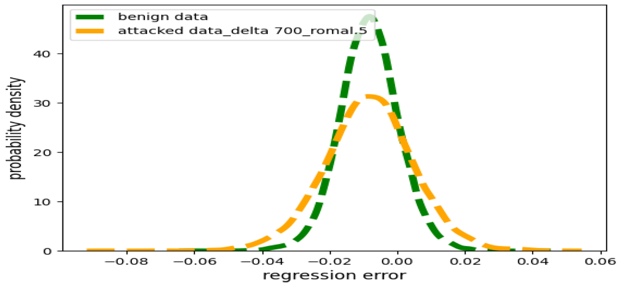
Large Strength Poisoning Attacks: Figure 3 shows a contaminated distribution of resulting from a large data poisoning attack we implemented using (i.e., 7 times more in strength than the small poisoning attack) and , compared to the benign distribution.
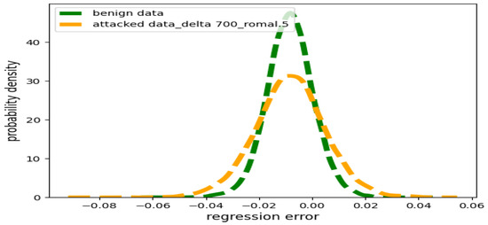
Figure 3.
Benign distribution of errors versus contaminated distribution under large poisoning .
In Figure 3, the green line depicts the distribution of regression errors that correspond to the benign portion of the training dataset, and closely approximates a normal distribution () verified via the K-S test. On the other hand, the yellow line depicts the distribution of regression errors that correspond to the attacked portion of the training dataset from the RUC latent space where the poisoning attack has large . Performing a K-S test on the yellow perturbed distribution, we found it fits closely with the student t-distribution. This disparity requires us to consider the variability introduced by larger attacks and corresponding regression error distributions, differently than the case of smaller poisoning attacks.
In the least favorable distribution, the two components of the compound distribution, and G, are distinctly separated by ; i.e., each exhibiting a distinctly different shape.
In contrast, the parametric form of t-distribution seamlessly blends both and G into a single distribution with heavy tails [17,23].
The prominent impact of this larger poisoning attack strength results in the emergence of a different type of contaminated distribution represented by in Equation (13). We can represent the set as an inclusive range of contaminated distributions arising from various attack types, each introducing different levels of contamination, ranging from small to large perturbations. This set is defined as follows:
The probability density function (pdf) of the student t-distribution, with an auxiliary scale correction, can be expressed as follows:
Here, the gamma function is denoted as , represents the degrees of freedom, is the regression error, and represents the scale parameter in the t-distribution. Thus, the likelihood function for the t-distribution, considering all N training data points, is
Since maximizing the likelihood function is equivalent to minimizing the log-likelihood function, taking the negative natural logarithm of Equation (15) yields
In general, the parameter estimate via MLE, just like in the earlier case, is found by the following empirical risk minimization problem:
In our problem, we deal with a single statistically variable parameter, and we sample residual values within a window. In the t-distribution, the degrees of freedom indicate that smaller values result in heavier tails, while larger values make it resemble a Gaussian distribution. Considering these factors, choosing a smaller for the degrees of freedom is appropriate for larger attacks, as shown in Figure 3. Hence, replacing in Equation (16), and using the algebra and derivation shown in Appendix B, by taking the derivative of Equation (16) with respect to and then integrating, we obtain the following solution according to M-estimation theory:
The above equation, in fact, matches the so-called Cauchy–Lorentz Loss Function from the class of M-estimator functions, which explains why we choose this loss function for resilient threshold learning [22].
Significance: The significance of the above analysis is that the mitigation resulting from resilient learning in anomaly detection can be performed by implementing different kinds of attack strategies and checking the contaminated distribution’s nature and derive the corresponding optimal estimator that will produce the minimax estimate under such attacks.
5.2. Robust Learning Algorithms for Detection Threshold
While the previous section was dedicated to theoretically estimating the best loss function for learning under different types of attacks, this section is about how to use the identified appropriate estimators to propose a resilient threshold learning algorithm for time series anomaly detectors that is robust under the presence of data poisoning attacks during the training. Specifically, we combine the benefits of quantile-weighted regression with the robust Cauchy and Huber loss functions for learning the thresholds.
This results in two new threshold learning algorithms: (a) Quantile-Weighted Regression with Huber Loss (Algorithm 2), and (b) Quantile-Weighted Regression with Cauchy Loss (Algorithm 3). In our experiments, we compare these with classical (unweighted/non-quantile) regression with Cauchy loss and unweighted regression with Huber loss, with pseudo-code provided in the preliminary version of this work [9].
| Algorithm 2: Quantile-Weighted Regression with Huber loss () |
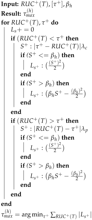 |
For the algorithms, we provide the pseudocode for learning the upper threshold , since the same process applies to learning . For learning , the algorithm remains the same except that it runs with inputs and parameter .
For optimal learning of , the input training samples are , and the search space for the candidate parameter is for each algorithm. We begin by explaining Algorithm 2, which uses Huber loss and modified quantile-weighted regression (to handle heteroskedasticity). The regression error is defined as the difference . Quantile regression applies different weights to the regression error depending on whether the candidate parameter fit is greater or lesser than the input points. This approach is necessary to reduce false alarms since the distribution of samples is not Gaussian, violating the assumptions of ordinary least squares regression.
We select a candidate for the upper threshold and compare whether it is greater or less than each point in the set . If , we assign it a weight and calculate the corresponding weighted regression errors, denoted as . Otherwise, if , we assign the regression error a weight , where . To embed the Huber estimator, for each weighted error , we calculate a loss value according to the Huber loss, depending on whether is greater or less than . This procedure gives an value for each training data point in the set for a fixed .
The empirical loss value for a single candidate is the sum of values over each entry in the set , denoted as . Each candidate generates a unique . The final optimal estimate is the that minimizes , as shown in the last line of Algorithm 2.
In a similar manner, we describe Algorithm 3, which uses the Cauchy loss instead of Huber, while keeping everything else the same. The only difference is the calculation of from the weighted regression error , based on how the Cauchy loss transforms the error into a loss value. The optimal solution is denoted as , indicating that the Cauchy loss function was used for learning the upper threshold.
| Algorithm 3: Quantile Weighted with Cauchy loss () |
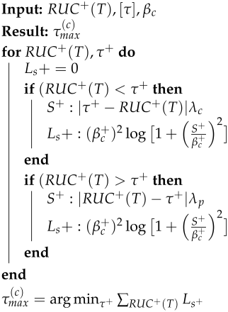 |
When no asymmetric weights are applied to the regression errors, Algorithms 2 and 3 have been rewritten for Huber and Cauchy losses, respectively, using similar logic. In each case, we are only learning the bias parameter without the slope, as we want a fixed, time-independent threshold for flagging an anomaly.
5.3. Learning Hyperparameters
Now, we discuss the selection of the scaling hyperparameters of the loss functions, and , and the hyperparameters of the weighted quantile regressors, and , over a cross-validation set. The search space for and is bounded between 0 and the extremum of the set or , and is between 0 and 1, with less than .
We partitioned the first 3 months of the 2016 dataset and used several values of the scaling hyperparameter, with a feasible range dictated by the regression errors (i.e., ) as discussed in the previous subsection. We tested several combinations of in each partition, selected the best one using the objective in Equation (19), and averaged the results.
For all results, we kept and . The weight assignment reflects that reducing false alarms is more than half as important. We minimized the joint false alarm (FA) and missed detection (MD) rates in the cross-validation sets. We used a coordinate grid search method over the cross-validation set to learn the best hyperparameters. This process was performed across various combinations of attack scales and strengths. After obtaining the optimal value for each loss function across all attack scales and strengths, we calculated the average across these attack combinations for each loss.
5.4. Theoretical Results and Explainability
This section is dedicated to the proof of correctness of experimental results. Often, some papers implement a robust learning approach and report the performance but that does not prove correctness of experimental observations because experiments/codes may have biases/bugs which may alter conclusions. Therefore, it is imperative that researchers give theoretical proofs to prove correctness of experiments and its conclusions.
In the previous section, we showed the relationship between poisoning attacks, their influence on the distribution of regression errors, and how should inform the loss function choice. Now, we theoretically prove that in the presence of poisoning attacks with varying degrees of perturbation, which loss function provides better mitigation and why—which addresses an important aspect of machine learning, i.e., the explainability aspect. In the experimental section, we show that the theoretical results match the experimental result, which is a proof of correctness of the experimental findings.
Consider regression error data points where for , and is the hyperparameter of the loss function. The regression error data points are classified into two categories based on the hyperparameter . Among the N data points, those that exceed are categorized as “large errors”, while those that fall within the range of to are categorized as “small errors”.
Consequently, we can express this situation as follows: Out of the N data points, m have regression errors greater than (, where ), and the remaining data points have errors within the interval to (, where ). Thus, the perturbed errors are those either greater than or within the range of to . It is important to observe that in the context of RSL attacks, adversaries introduce perturbations of varying strength, either small or large, into training data points. This leads to distinct sets of regression errors following different distributions, as described by Equation (13). In reality, knowing the type and characteristics of attacks a priori is not straightforward, so the choice of the best loss function remains unclear. To compare the performance of different loss functions, we present an analysis based on Influence Functions (IFs) and Mathematical Induction.
Comparing the Influence Functions (IFs) of the Cauchy and Huber estimators, the estimator with the smaller IF under perturbations is less affected by attacks and thus more robust. To maintain broad applicability, we can make an initial assumption about the regression error data points, denoted as and parameterized by . We aim to progressively extend this assumption and demonstrate its validity.
Let , , and ; the following inequality holds true:
then the above means that and, hence, Cauchy provides more mitigation compared to Huber. In contrast, if , then the Huber loss would provide more mitigation than Cauchy. This comparison indicates that the effectiveness of these robust loss functions in mitigating the influence of outliers depends on their relative Influence Functions.
This assumption shows that any perturbation in individual data points has a smaller effect on the Influence Function (IF) of Cauchy compared to Huber. In Equation (20), we can distinguish between two categories of regression errors: those considered small and those classified as large. This differentiation can be expressed as follows:
- If , i.e., big residual
- If , i.e., small residual
We employ a direct inductive proof in this analysis. We start by examining a single data point, denoted as , and determine whether the inequality in Equation (20) holds. Then, we generalize it for multiple points based on the conditions of our problem.
Let with . Depending on whether (large) or (small), we provide a direct proof using Equations (21) and (22). A positive error can fall into either category, large or small. Case 1: considers the scenario where the residual is large. We begin by proving the inequality for a single point using Equation (21), and then generalize the argument to multiple points. Case 2: addresses the case of small errors. We similarly start with a single point and extend the proof to multiple points using Equation (22). Finally, we consider Case 3: where both large and small errors occur simultaneously (which is the practical casr) and prove which influence function yields a lower value. Thus, the complete set of cases is as follows:
Case 1: If , big regression error, then :
The left side is always negative since and , while the right-hand side is positive. Thus, our assumption (i.e., ) holds for large regression errors.
For the case where (a large regression error), we will show that the opposite statement, , is false through proof by contradiction.
However, the last inequality is logically impossible because squared terms cannot be smaller than negative terms. Assuming the opposite leads to a mathematical contradiction. Thus, when (indicating a large regression error), with and . Hence, we proved that the Cauchy loss function mitigates the impact of poisoning more effectively than the Huber loss for bigger residuals which happen under poisoning.
Generalization to Multiple Big Regression Errors: Now, suppose there are a total of m large errors , where (). Given these m large errors, we have m inequalities of the form
Applying generalized Triangle Inequality leads to the following:
This inequality is valid because the total value on the left-hand side is smaller than the total value on the right-hand side. The reasoning behind this is that each individual term on the left is minimized due to the properties of the generalized Triangle Inequality, which effectively bounds the summation when compared to the sum of the signs of the larger errors on the right.
Case 2: If small regression error, then suppose or greater. Hence, . Then, we can write
Our demonstration has shown that, when dealing with small errors, the IF of Cauchy is less than that of Huber, indicating that the Cauchy loss function is either better than or equal to Huber under small poisoning attacks.
Generalization to Multiple Small Regression Errors: Now, consider the case of small regression errors where , (). Given a total of small errors, we have inequalities of the form
Applying the generalized Triangle Inequality, we combine the above inequalities and derive a new inequality. For all (), the following holds true:
The above indicates that, in the presence of very small attacks, both the Cauchy and Huber loss functions provide equally effective mitigation in predicting the detection thresholds.
Case 3: Mixed Regression Errors (Large and Small). We consider the scenario where both large and small errors are present simultaneously (real world case study) and prove which influence function yields a lower value.
Previously, we showed that Equation (13) represents the distributions affected by , resulting from various attack types. In real-world scenarios, whether results from a large or small poisoning attack, it causes both small and large perturbations in regression errors. The key difference is the ratio of small to large errors. For instance, a large attack strength leads to a higher number of large regression errors compared to small errors. Thus, in real-world scenarios, we need to combine inequality Equations (23) and (24) by using a similar technique that involves summing the two sides of these inequalities. As a result, Equation (20) holds for all small and large regression errors , i.e.,
The analysis reveals that the Cauchy loss has a lower IF compared to the Huber loss function when both small and large errors are present due to attacks and benign fluctuations. Based on this, it is explainable that the Cauchy loss function is more effective for the greedy case where the attacker seeks to launch larger data poisoning strengths to quickly inflict maximum damage. However, the experiments also reveal a trade-off related to the low base rate probability of a poisoning attack occurring that reveals a deeper scientific question.
5.5. Security Evaluation Metrics
Unlike previous works, we used two novel metrics for security evaluation, instead of popular metrics such as false alarm rate, missed detection rate, ROC curves, and precision, recall. This deliberate avoidance is following the recommendations by NIST [2] for security evaluation of time series anomaly-based attack detectors.
When it comes to cybersecurity of critical CPS infrastructure, detection rate should not be used as a way to test the goodness of a defense. This is because the algorithms are public, so attackers can always come up with a poisoning strategy that does not violate the robust/resilient thresholds and escape detection. In that case, the detection rate is zero. However, it does not prove the effectiveness of the cybersecurity/mitigation strategy. Rather, what really proves effectiveness of the security mitigation is if we can prove that the impact of undetected attack is small or limited when an evasion attack that just bypasses the learned robust threshold during training is applied by the attacker during the testing. Hence, we use impact of undetected attack as one the metrics of security evaluation while evaluating our work’s effectiveness in the test set.
Another key concern is the false alarm rate and why it is misleading to use false alarm rates for time series detectors like ours which frequently check for attacks (not one time check). Suppose a cybersecurity mitigation has a false alarm rate of 1%. If the detector runs every second, then 1% false alarm rate will yield 864 false alarms in a single day (clearly unusable practically) if there are no actual attacks. However, if the detectors runs per hour of the day, the same 1% false alarm rate in the same scenario produces on average at least two false alarms per day (more usable but still poor). Given that the prior probability of an actual attack is much lower than the benign condition, such false frequencies and rates become even more misleading. As is clear from the above discussion, it is proven that false alarm rates are inappropriate for cybersecurity mechanisms that operate on streaming data because it does not give any idea on the usability of the approach. This is well known from Axelsson et. al.’s seminal work on the flaws of cybersecurity detection metrics [24]. From the above explanation, it is clear that the usage of ROC curves, false alarm, missed detection, and precision, recall is misleading and should be avoided. Hence, NIST recommends not to use false alarm rates for cybersecurity approaches that run frequently on streaming data. Rather, the expected (average) time between consecutive false alarms which incorporates the notion of time and gives a better sense of whether the cybersecurity mechanism produces false alarms at a frequency that is practical and usable. The larger the average time gap between any two false alarms, the better it is because the number of costly disruptions and host-based security audits needed is going to be lesser.
Impact of Undetected Attack: The effectiveness of integrity violations is quantified through the impact of undetected attacks on the utility after applying our attack and defense mechanisms [2]. To calculate the impact of undetected attacks per day, we use lost revenue, denoted by , in terms of the unit price of electricity:
where is the number of reports per day, is the average per unit (KW-Hour) cost of electricity in the USA, is the margin of false data in the test set, and M is the number of compromised smart meters in the test set. The impact of undetected attack is as follows:
is the time difference between attack start and end of the test set in days. Lesser indicates better mitigation.
Expected Time between Consecutive False Alarms: Instead of the well-known false alarm rate, we use the expected time between two false alarms to evaluate false alarm performance. The is a NIST [2] recommended metric to avoid base rate fallacy in the reported performance false alarm performance for time series anomaly based detection for cybersecurity:
where is the number of false alarms, and is the time gap between two false alarms. If there is only one false alarm, is set to 364, assuming another false alarm is likely within a year. A lower indicates worse performance.
6. Experimental Evaluation
For the experimental evaluation, our proof of concept is a dataset from the Pecan Street project [25] containing hourly power consumption from 200 smart meters over three years (2014, 2015, 2016) divided into training, cross-validation, and testing. The training data includes all records from 2014 and 2015, as in previous work [1], to ensure fair performance. The remaining records from 2016 are divided into two parts for cross-validation and testing. All records from the first three months of 2016 are used for cross-validation, while the remaining nine months are used as the test set. The hyperparameters and , learned through cross-validation, were found to be and , respectively. For each loss function and regression type, we measure performance based on the impact of undetected attacks as a function of the following attack variables: (1) poisoning attack strength and scale , and (2) evasion attack strength and scale .
Furthermore, while reporting performance we use different acronyms that denote the threshold learning algorithm that includes both regression type and loss function. These acronyms are described in Table 1. The algorithmic procedure for regular (i.e.) non quantile versions of the NQC and NQH can be found in our preliminary conference version [9].

Table 1.
Acronyms for design choices.
RSL Poisoning Implementation Details: For RSL poisoning attack, we varied poisoning margin between 50 and 300 and varied between 20 and , and the RSL attack duration was between 1 April and 30 June 2014.
RSL Evasion Implementation Details: To investigate performance in the test set, we crafted attacks with varying percentages of compromised meters and varying data perturbation margins . The combinations were selected such that none of the attacks exceeded the learned standard limit, allowing us to measure the impact of undetected attacks. In the test set, we varied between 20 and , and between 10 and 400, covering a wide range of attack intensities.
To remove bias in performance, we launched evasion attacks on three distinct 90-day time frames in 2016. The reported IMPACT (USD) in each result is the average impact of undetected attacks per 90-day frame, across the three attack time frames.
Performance evaluation of Robustness: For comparative performance evaluation, we compare all loss function choices by grouping them into two categories: (a) within quantile-weighted regression and (b) within unweighted regression. We select the best-performing loss function from each group and compare their performance to determine which loss function type and regression type is most robust against a given attack.
Performance is measured in terms of the mean impact of undetected attacks per 90 days (I) (when there is an evasion attack in the test set) and the expected time between false alarms () (when there are no attacks in the test set). The impact of an undetected attack is influenced by (i) poisoning attack strength and (ii) evasion attack strength. Therefore, we use these two attack parameters to measure how the impact of undetected attacks varies across loss functions and regression choices.
6.1. Evaluating Impact of Undetected Attacks
This subsection is dedicated to all results related to impact of undetected attacks in the test set as a result of data poisoning, given that we assume the attacker knows the threshold and is never detected.
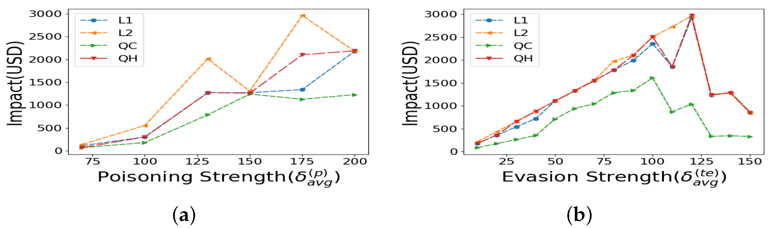
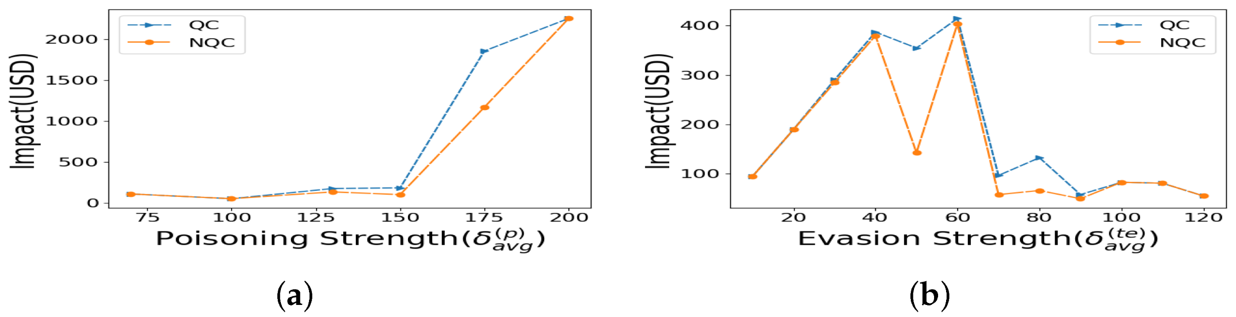
Now, we discuss loss function choices with asymmetric weighting of positive versus negative regression errors, which is our proposed framework. Figure 4a shows that across various poisoning strengths (), the QC loss function consistently results in equal or lower attack impact across all loss function choices. The evasion attack strength is , with a scale of , which bypasses detection assuming the attacker has complete knowledge of our method.
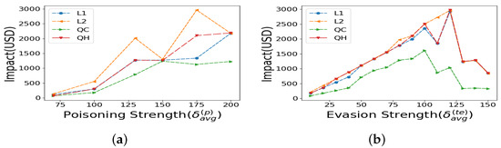
Figure 4.
Impacts under quantile regression over (a) varying poisoning attack strength, (b) varying evasion attack strength.
Next, we vary the evasion strength to evaluate performance. In Figure 4b, we observe that, across various evasion attack strengths, the QC loss function results in a lower impact compared to all other loss function choices. The poisoning attack strength is and the scale is for Figure 4b.
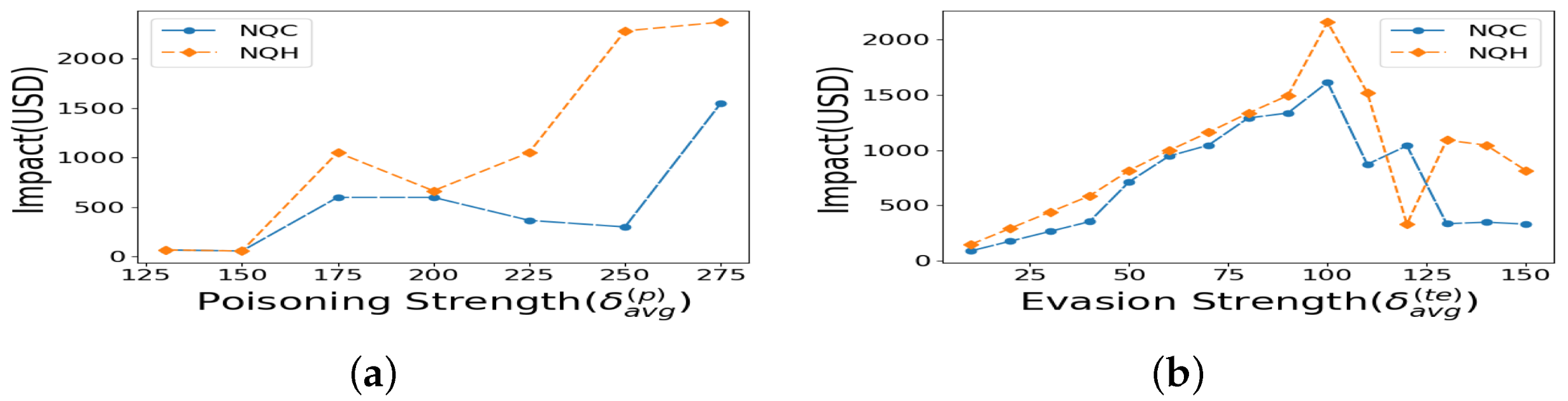
Effect of Loss function choice Here, we show the impact the loss function choice alone had on the resilient learning without Quantile weights used in the learning. Figure 5a indicates that, across different poisoning attack strengths , the NQC (unweighted Cauchy Loss) is equal to or lower in impact than NQH. The evasion attack strength is and the scale is . In contrast, for a poisoning attack with and , Figure 5b shows the impact across all evasion strengths , and proves that the NQC is lower in impact than NQH.
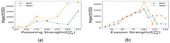
Figure 5.
Impacts under unweighted regression: (a) varying poisoning attack strength, (b) varying evasion attack strength.
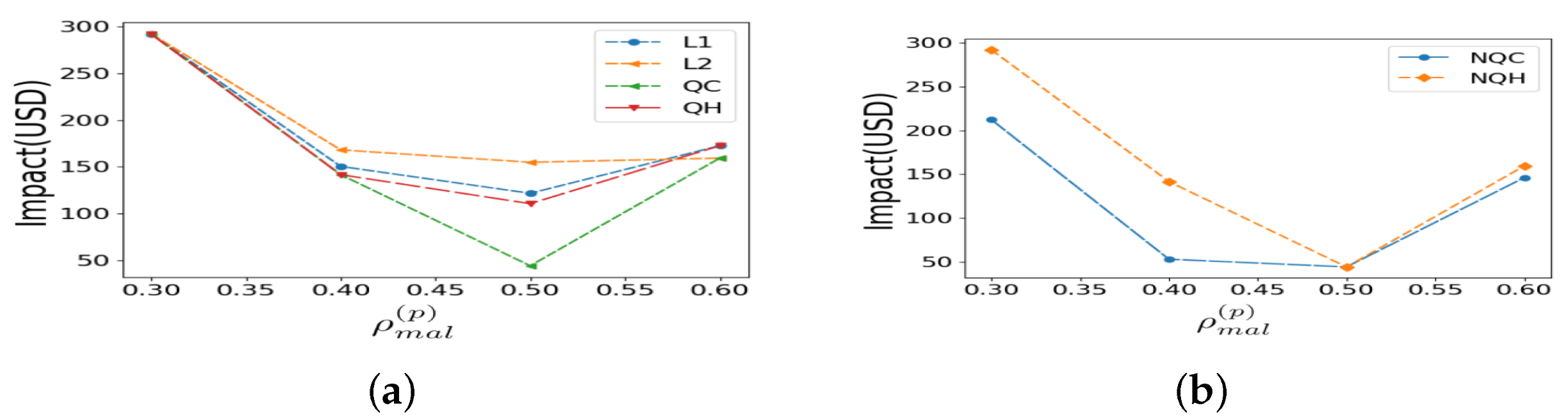
Impact of Quantile Weights’ Choice Next, we compare the winning loss function, Cauchy, in both quantile regression and regular (non-quantile) in Figure 6a,b. It is important to isolate the effect that quantile weights have on the mitigation, keeping the same most robust loss function. We find that regular Cauchy performs better in minimizing the impact of undetected attacks. This might lead the hasty conclusion that quantile-weight Cauchy loss is less optimal than regular Cauchy. However, this is counterintuitive, because later in Table 2, we show that the false alarm performance of NQC is poorer. Due to base rate paradox, the false alarm performance should get higher priority due to imbalanced prior probability of not having a poisoning. Hence, we should use quantile Cauchy, even though the non-quantile has less impact of undetected attack, because using quantile cauchy gives jointly better and I.
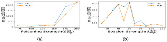
Figure 6.
Quantile versus regular regression with Cauchy: (a) poisoning strength, (b) evasion strength.
Table 2.
Expected time between false alarms: no test set attacks.
Figure 6a shows that the impact of NQC is either equal to or lower than the impact of QC for varying poisoning strength for a representative evasion attack with and . Similarly, Figure 6b shows either equal or lower impact of performance for NQC than the impact of QC for varying evasion attack for a representative poisoning attack with and . The results clearly indicate that the NQC loss function outperforms all other loss functions in terms of impact of undetected.
Impact versus Varying Attack Scale: We want to determine if the conclusions change when is adjusted. Figure 7a shows that the QC is either equal to or lower in impact than all other loss functions. Similarly, Figure 7b shows that the NQC is either equal to or lower in impact than NQH. For both Figure 7a,b, the poisoning attack strength is and the evasion strength is .
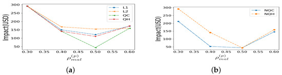
Figure 7.
Impact versus attack scale: (a) QR, (b) NQR.
6.2. Evaluating False Alarm Performance with Base Rate Effects
In this subsection, we analyze the expected time between false alarms under two variations. First, we examine the expected time between two consecutive false alarms with training data poisoning, but there is no attacks launched in the test set. The question we are asking here is whether this occurrence causes an increase in false alarm due to the design response of using robust ML principles for anomaly detection criterion. Second, we measure the expected time between two consecutive false alarms with no poisoning attacks in the training set and no data falsification attacks in the test set as well—we call this base rate ETFA. This is important because this is the most probable scenario and important to verify that the fear of poisoning attacks that led to a more resilient algorithm does not cause degradation of system usability (that is negatively affected by increased false alarm).
Expected Time Between False Alarms with No test set attacks: To measure the expected time between false alarms, we used the annual base rate of false alarms in the test set when there were no attacks throughout 2016. This is because the false alarm rate is typically highest when no attacks are present, given that poisoning was part of the training set. Table 2 presents the expected time between false alarms for various loss functions in the presence of an RSL poisoning attack and shows that the quantile Cauchy loss yields worse false alarm performance compared to other design choices. The quantile version of Cauchy performs slightly better than the non-quantile version.
Base Rate Paradox Trade-off under No Poisoning: Table 3 shows the expected time between false alarms in the test set, when there is no data poisoning during training. Note that the base rate probability of a poisoning attack occurring is very low. The quantile Cauchy loss has poor false alarm performance, generating one false alarm every 45 days. On the other hand, the quantile Huber is as good as quantile L2, generating a false alarm every 364 days.
Table 3.
False alarm performance: no poisoning attacks.
An interesting trade-off is that using robust loss functions comes at the cost of increased false alarms, especially when the low base rate of poisoning is considered. Therefore, while adopting a robust loss function, this trade-off should be considered, and the weights during cross-validation may need to be adjusted accordingly. Our recommendation is that quantile Huber is the best choice, even though quantile Cauchy is theoretically more robust to poisoning attacks. When a poisoning attack does occur (though its probability is low), quantile Huber performs better than the more popular quantile L1 and L2 loss functions.
6.3. System Complexity and Performance Discussion
Here, we discuss the model size and complexity of learning.
Model size: There are two parameters for threshold learning—the upper and the lower detection threshold and two hyperparameters of the Cauchy/Huber loss function (i.e., the scaling hyperparameter in the M-estimator) as applied to the learning of upper and lower threshold learning. Hence, the model size is small.
Complexity: The method is very lightweight in storage complexity. It only stores threshold values and regression parameters, making it highly suitable for resource-constrained environments. Regarding computational time complexity, the RUC generation scales linearly with the size of the input data . On the other hand, the threshold learning that uses a Cauchy loss is a convex and differentiable, unlike quantile L1. Hence, gradient descent applies with a known complexity of , where k is the number of iterations needed, n is the number of samples, and d is the number of features. Since our learning of attack detection threshold needs only a single feature (i.e., the RUC latent space), the complexity of the robust learning is . Per iteration, the complexity is , which also gives the importance of using latent representation metric (i.e., RUC). The number of iterations depends on the step size and it is an arbitrary choice of the designer. However, since the RUC metric space is sparse and contains small numbers between −1 and +1 in range, the number of iterations will not cause a performance bottleneck.
7. Conclusions
This paper proposed two robust approaches for learning the threshold of time series anomaly-based attack detection, with theoretical justification for the experimental results, using a smart metering infrastructure as a proof of concept. Our approach involved robust loss functions, including Cauchy and Huber, applied to quantile and unweighted regression errors. Through comprehensive analysis, we theoretically assessed the security performance of these methods, determining their suitability for different attack strengths. Additionally, we emphasized the crucial role that data point distribution plays in selecting the appropriate loss function for learning thresholds and its relation to security performance. We validated our findings through experimental assessments using metrics such as the impact of undetected attacks and the expected time between false alarms, both well suited for evaluating security under advanced persistent threats. Our results indicate that, in terms of impact robustness, Cauchy outperforms the more widely known Huber loss function, especially under moderate to high attack strengths. However, when accounting for the base rate fallacy, quantile-weighted Huber loss emerges as a more effective choice for reducing false alarm occurrences.
Author Contributions
Conceptualization, S.B.; Methodology, S.B.; Software, S.A.; Validation, S.A.; Formal analysis, S.A.; Data curation, S.A.; Writing—original draft, S.A.; Writing—review & editing, S.B.; Supervision, S.B.; Funding acquisition, S.B. All authors have read and agreed to the published version of the manuscript.
Funding
The research was supported by USA’s National Science Foundation (NSF) grants, OAC-2320951, CNS-2030611.
Institutional Review Board Statement
Not applicable.
Informed Consent Statement
Not applicable.
Data Availability Statement
The data presented in this study are available on request from the corresponding author.
Acknowledgments
We thank Mohammad Jaminur Islam for assistance with experiments.
Conflicts of Interest
The authors declare no conflicts of interest. The funders had no role in the design of the study; in the collection, analyses, or interpretation of data; in the writing of the manuscript; or in the decision to publish the results.
Appendix A
In order to estimate the location parameter of least favorable distribution () in Equation (8), we need to find an M-estimator that solves the empirical risk minimization problem in Equation (11). Mathematically, we define the problem for all training data points : minimizing the log-likelihood function is equivalent to finding the solution to
In fact, is simply the Influence Function (IF) of an M-estimator under the least favorable distribution, where the IF serves as the parametric choice for learning the estimate.
From the above equation, let be a scaling hyperparameter. The M-estimator for the location parameter of the least favorable distribution (), which aligns with this IF, is the Huber M-estimator or Huber loss function [17,18]. By plugging the above equation into the integral, we obtain
The above integral matches a known form in the class of M-estimators called Huber loss function [26]:
where denotes the regression error between a data point and a parameter candidate, is the scaling hyperparameter for Huber loss. The Huber loss is a combination of and norms, as evident from the two conditional equations. For smaller regression errors , where , they contribute to the squared error in the empirical loss, while large regression errors are proportional to the absolute error in the empirical loss. This causes the Huber loss function to grow quadratically for errors smaller than or equal to , and linearly for errors larger than .
Appendix B
In order to estimate the location parameter of the t-distribution () in Equation (14), we need to find an M-estimator that solves the empirical risk minimization problem in
Considering the degrees of freedom , the derivative of Equation (16) is the Influence Function (IF) of the M-estimator. The use of the t-distribution as a parametric choice for estimating the location parameter is outlined below, as described by [23]: for all training data points ,
The definition of degrees of freedom in the t-distribution indicates that smaller values result in heavier tails, while larger values make it resemble a Gaussian distribution. Thus, selecting for the degrees of freedom is appropriate.
Large regression errors significantly impact the Influence Function (IF) for the location estimator . However, these large residuals have less effect on the estimated value of when using the t-distribution as the parametric choice for the maximum likelihood estimator (MLE) and IF. Thus, by substituting into Equation (16), we obtain the appropriate IF for our purpose:
Here, is the scaling parameter.
In order to determine the most suitable estimator for our specific problem, we must integrate the IF with respect to . This approach follows the principles of robust estimation theory. By integrating Equation (A7) and applying the auxiliary scale correction, we arrive at the following result:
If we define , it can be demonstrated that . By substituting this expression back into the integral and replacing the value of u, we find the following result:
The above expression is documented in computer vision literature as the Cauchy–Lorentzian loss function. The above loss function discussed in [27] is acknowledged as a lesser-known estimator function within the category of M-estimators. Its mathematical representation is defined as follows:
where represents the respective errors and serves as the scaling hyperparameter associated with the Cauchy loss, .
Equation (A10) represents a scaled norm. It is commonly assumed that Huber loss is preferable due to its linear growth for large residuals, as it is often seen as more robust. However, in this specific case study, both theoretical analysis and experimental findings revealed a counterintuitive result: Cauchy loss outperformed Huber loss in terms of resilience against poisoning attacks.
References
- Bhattacharjee, S.; Das, S.K. Detection and Forensics against Stealthy Data Falsification in Smart Metering Infrastructure. IEEE Trans. Dependable Secur. Comput. 2021, 18, 356–371. [Google Scholar] [CrossRef]
- Urbina, D.; Giraldo, J.; Cardenas, A.A.; Tippenhauer, N.; Valente, J.; Faisal, M.; Ruths, J.; Candell, R.; Sandberg, H. Survey and New Directions for Physics-Based Attack Detection in Cyber-Physical Systems. ACM Comput. Surv. 2018, 51, 1–36. [Google Scholar]
- Islam, J.; Talusan, J.P.; Bhattacharjee, S.; Tiausas, F.; Vazirizade, S.M.; Dubey, A. Anomaly based Incident Detection in Large Scale Smart Transportation Systems. In Proceedings of the 2022 ACM/IEEE 13th International Conference on Cyber-Physical Systems (ICCPS), Milano, Italy, 4–6 May 2022; pp. 215–224. [Google Scholar]
- Goodfellow, I.; Shlens, J.; Szegedy, C. Explaining and harnessing adversarial examples. arXiv 2015, arXiv:1412.6572. [Google Scholar]
- Domingos, N.D.P.; Mausam, M.; Sanghai, S.; Verma, D. Adversarial Classification. In Proceedings of the KDD04: ACM SIGKDD International Conference on Knowledge Discovery and Data Mining, Seattle, WA, USA, 22–25 August 2004. [Google Scholar]
- Yu, Y.; Xia, S.; Lin, X.; Kong, C.; Yang, W.; Lu, S. Toward Model Resistant to Transferable Adversarial Examples via Trigger Activation. IEEE Trans. Inf. Forensics Secur. 2025, 20, 3745–3757. [Google Scholar] [CrossRef]
- Available online: https://www.miningreview.com/top-stories/research-study-quantifies-energy-theft-losses/ (accessed on 1 January 2020).
- Tian, Z.; Cui, L.; Liang, J.; Yu, S. Comprehensive Survey on Poisoning Attacks and Countermeasures in Machine Learning. ACM Comput. Surv. 2023, 55, 166. [Google Scholar] [CrossRef]
- Bhattacharjee, S.; Islam, J.; Abedzadeh, S. Robust Anomaly based Attack Detection in Smart Grids under Data Poisoning Attacks. In Proceedings of the ACM Asia’CCS Workshop on Cyber Physical Systems Security (ACM CPSS), Nagasaki, Japan, 30 June 2022. [Google Scholar]
- Jiraldo, G.; Cardenas, A. Adversarial Classification under Differential Privacy. In Proceedings of the Network and Distributed Systems Security (NDSS) Symposium, San Diego, CA, USA, 23–26 February 2020. [Google Scholar]
- Jaglieski, M.; Oprea, A.; Liu, C.; Rotaru, C.; Li, B. Manipulating Machine Learning: Poisoning Attacks and Countermeasures for Regression Learning. arXiv 2018, arXiv:1804.00308. [Google Scholar]
- Ghafouri, A.; Vorobeychik, Y.; Koutsoukos, X. Adversarial Regression for Detecting Attacks in Cyber-Physical Systems. In Proceedings of the Twenty-Seventh International Joint Conference on Artificial Intelligence (IJCAI-18), Stockholm, Sweden, 13–19 July 2018. [Google Scholar]
- Tramer, F.; Kurakin, A.; Papernot, N.; Goodfellow, I.; Boneh, D.; McDaniel, P. Ensemble adversarial training: Attacks and defenses. arXiv 2018, arXiv:1705.07204. [Google Scholar]
- Oluyomi, A.; Bhattacharjee, S.; Das, S.K. Detection of False Data Injection in Smart Water Metering Infrastructure. In Proceedings of the 2023 IEEE International Conference on Smart Computing (SMARTCOMP), Nashville, TN, USA, 26–30 June 2023; pp. 267–272. [Google Scholar]
- Roy, P.; Bhattacharjee, S.; Das, S.K. Real Time Stream Mining based Attack Detection in Distribution Level PMUs for Smart Grid. In Proceedings of the GLOBECOM 2020–2020 IEEE Global Communications Conference, Taipei, Taiwan, 7–11 December 2020. [Google Scholar]
- Urbina, D.I.; Giraldo, J.A.; Cardenas, A.A.; Tippenhauer, N.O.; Valente, J.; Faisal, M.; Ruths, J.; Candell, R.; Sandberg, H. Limiting the Impact of Stealthy Attacks on Industrial Control Systems. In Proceedings of the CCS’16: 2016 ACM SIGSAC Conference on Computer and Communications Security, Vienna, Austria, 24–28 October 2016; pp. 1092–1105. [Google Scholar]
- Filipovic, V. System Identification using Newton–Raphson Method based on Synergy of Huber and Pseudo–Huber Functions. Autom. Control Robot. 2021, 20, 87–98. [Google Scholar] [CrossRef]
- Shevlyakov, G.; Kim, K. Huber’s Minimax Approach in Distribution Classes with Bounded Variances and Subranges with Applications to Robust Detection of Signals. Acta Math. Appl. Sin. 2005, 21, 269–284. [Google Scholar] [CrossRef]
- Reinhardt, H.E. The Use of Least Favorable Distributions in Testing Composite Hypotheses. Ann. Math. Statist. 1961, 32, 1034–1041. [Google Scholar] [CrossRef]
- Lehmann, E.L. Reminiscences of a Statistician: The Company I Kept; Springer: New York, NY, USA, 2008. [Google Scholar]
- Huber, P.J. Robust Estimation of a Location Parameter. Ann. Math. Stat. 1964, 35, 73–101. [Google Scholar] [CrossRef]
- Zhang, Z. Parameter estimation techniques: A tutorial with application to conic fitting. Image Vis. Comput. 1997, 15, 59–76. [Google Scholar] [CrossRef]
- Sumarni, C.; Sadik, K.; Notodiputro, K.A.; Sartono, B. Robustness of Location Estimators Under t-Distributions: A Literature Review; IOP Conference Series: Earth and Environmental Science; IOP Publishing: Bristol, UK, 2017; Volume 58. [Google Scholar]
- Axelsson, S. The base-rate fallacy and the difficulty of intrusion detection. ACM Trans. Inf. Syst. Secur. 2000, 3, 186–205. [Google Scholar] [CrossRef]
- Pecan Street Project Dataset. Available online: https://www.pecanstreet.org/ (accessed on 1 January 2020).
- Huber, P.; Ronchetti, E. Robust Statistics; Wiley Probability and Statistics: Hoboken, NJ, USA, 2009; ISBN 978-0470129906. [Google Scholar]
- Li, X.; Lu, Q.; Dong, Y.; Tao, D. Robust Subspace Clustering by Cauchy Loss Function. IEEE Trans. Neural Netw. Learn. Syst. 2019, 30, 2067–2078. [Google Scholar] [CrossRef] [PubMed]
Disclaimer/Publisher’s Note: The statements, opinions and data contained in all publications are solely those of the individual author(s) and contributor(s) and not of MDPI and/or the editor(s). MDPI and/or the editor(s) disclaim responsibility for any injury to people or property resulting from any ideas, methods, instructions or products referred to in the content. |
© 2025 by the authors. Licensee MDPI, Basel, Switzerland. This article is an open access article distributed under the terms and conditions of the Creative Commons Attribution (CC BY) license (https://creativecommons.org/licenses/by/4.0/).