Application of the Adaptive Mixed-Order Cubature Particle Filter Algorithm Based on Matrix Lie Group Representation for the Initial Alignment of SINS

Abstract

Under large azimuth misalignment conditions, the initial alignment of strapdown inertial navigation systems (SINS) is challenged by the nonlinear characteristics of the error model. Traditional particle filter (PF) algorithms suffer from the inappropriate selection of importance density functions and severe particle degeneration, which limit their applicability in high-precision navigation. To address these limitations, this paper proposes an adaptive mixed-order spherical simplex-radial cubature particle filter (MLG-AMSSRCPF) algorithm based on matrix Lie group representation. In this approach, attitude errors are represented on the matrix Lie group SO(3), while velocity errors and inertial sensor biases are retained in Euclidean space. Efficient bidirectional conversion between Euclidean and manifold spaces is achieved through exponential and logarithmic maps, enabling accurate attitude estimation without the need for Jacobian matrices. A hybrid-order cubature transformation is introduced to reduce model linearization errors, thereby enhancing the estimation accuracy. To improve the algorithm’s adaptability in dynamic noise environments, an adaptive noise covariance update mechanism is integrated. Meanwhile, the particle similarity is evaluated using Euclidean distance, allowing the dynamic adjustment of particle numbers to balance the filtering accuracy and computational load. Furthermore, a multivariate Huber loss function is employed to adaptively adjust particle weights, effectively suppressing the influence of outliers and significantly improving the robustness of the filter. Simulation and the experimental results validate the superior performance of the proposed algorithm under moving-base alignment conditions. Compared with the conventional cubature particle filter (CPF), the heading accuracy of the MLG-AMSSRCPF algorithm was improved by 31.29% under measurement outlier interference and by 39.79% under system noise mutation scenarios. In comparison with the unscented Kalman filter (UKF), it yields improvements of 58.51% and 58.82%, respectively. These results demonstrate that the proposed method substantially enhances the filtering accuracy, robustness, and computational efficiency of SINS, confirming its practical value for initial alignment in high-noise, complex dynamic, and nonlinear navigation systems.

1. Introduction

The initial alignment is one of the key procedures in strapdown inertial navigation systems (SINS), and the accuracy of this alignment directly influences the overall performance and reliability of the system [1]. In the practical applications of autonomous underwater vehicles (AUVs), the initial alignment of SINS is typically required to be performed on a moving base, which places higher demands on alignment algorithms [2]. As the technological demands for SINS continue to rise, traditional alignment methods based on small misalignment angle error models and linear Kalman filtering approaches are gradually revealing limitations, particularly in complex environments. In adverse sea conditions, intense oceanic movements and environmental disturbances can result in a significant degradation in the heading accuracy of coarse SINS alignment, which further impacts the system’s navigational reliability and stability. As a result, how to achieve the high-precision initial alignment of SINS under large misalignment angles has become an urgent issue. In this context, the error dynamics of SINSs exhibit significant nonlinearity, making traditional linear filtering methods inadequate. Applying nonlinear filtering techniques is therefore crucial to improving the alignment accuracy and convergence speed of these systems.

In the context of pose estimation, rigid body rotation is one of the primary sources of nonlinearity in SINS. The main methods for representing rotational motion include Euler angles [3], rotation matrices, quaternions [4], and Lie algebras [5], each of which has its advantages and disadvantages. For instance, the Euler angle method is intuitive and easy to grasp, but it encounters the issue of gimbal lock when used in navigation calculations [6]. The rotation matrix method describes rotation using a 3 × 3 matrix but suffers from over-parameterization. The quaternion method is widely used for its excellent numerical stability, but it also suffers from over-parameterization and requires normalization at each filtering update to ensure that the quaternion remains unitary [7]. Using Lie algebra to represent poses in filtering methods resolves the over-parameterization issue and provides advantages in both algorithm convergence and pose estimation accuracy.

Currently, the commonly used nonlinear filtering methods include extended Kalman filtering (EKF), unscented Kalman filtering (UKF), cubature Kalman filtering (CKF), and particle filtering (PF) [8,9,10,11]. Particle filtering (PF) is widely used in applications such as target tracking and navigation [12], as it can handle state estimation problems in any nonlinear and non-Gaussian system, and has been extensively applied in these areas [13]. However, particle filtering faces two main challenges in practical applications: first, the challenge of selecting an appropriate importance density function, and second, the risk of particle degeneracy. Due to its superior numerical stability and filtering accuracy in high-dimensional systems, the importance density function for particle filtering can be generated by CKF instead [14]. However, during the initial alignment of a SINS on a dynamic base, state estimation is easily affected by gross measurement errors and state anomalies or outliers, which can result in significant degradation of the filtering accuracy and slower convergence when using traditional CPF algorithms.

To address the aforementioned issues, this paper proposes an adaptive mixed-order spherical simplex-radial cubature particle filter (MLG-AMSSRCPF) algorithm based on matrix Lie group representation. The algorithm innovatively uses the matrix Lie group SO(3) to represent attitude errors in manifold space, combining it with mixed-order spherical simplex-radial cubature Kalman filtering. It incorporates dynamic noise covariance adjustment, adaptive particle number, and particle weight update strategies, demonstrating a significantly improved filtering accuracy and computational efficiency. The system state variables consist of attitude errors represented by the Lie group matrix SO(3), velocity errors in Euclidean space, gyroscope drift errors, and accelerometer bias errors, which are accurately estimated within the framework of mixed-order cubature Kalman filtering. This algorithm establishes a mapping between Euclidean space and Lie group manifolds, allowing the volume points, state means, and variances of attitude errors to be computed in the tangent space of the manifold, while the velocity and other error variables are kept in Euclidean space. This approach avoids the complex Jacobian matrix solving process used in traditional extended Kalman filtering (EKF) and mitigates the potential issue of covariance non-positive definiteness that is found in unscented Kalman filtering (UKF).

Additionally, the algorithm introduces an adaptive noise covariance update mechanism which allows for the real-time dynamic adjustment of the noise covariance matrix based on the system’s noise characteristics, thereby significantly enhancing its adaptability to nonlinear systems in complex noise environments. Building upon this, the algorithm uses Euclidean distance to measure the similarity between particles, enabling adaptive adjustment of the particle number. This approach effectively alleviates the particle degeneracy problem while reasonably controlling the computational complexity [15]. Moreover, a multidimensional Huber loss function is introduced for the adaptive optimization of particle weights, effectively suppressing the influence of outliers on the weight distribution, which significantly improves the stability and robustness of the filter under complex noise conditions. In the initial alignment process of a SINS on a dynamic platform, the use of the MLG-AMSSRCPF algorithm can notably improve the alignment accuracy under large misalignment angle conditions, especially gross measurement errors and sudden changes in system noise are involved, demonstrating exceptional robustness and a rapid convergence capability. Beyond initial alignment tasks, the proposed algorithm also holds substantial potential for broader applications in attitude estimation and the navigation of vehicles such as autonomous cars and unmanned aerial vehicles (UAVs), where high precision and robustness are essential due to the system operating in real-world dynamic conditions.

• Main Contributions

  (1)

  Adaptive filtering framework based on matrix Lie group representation: An adaptive mixed-order spherical simplex-radial cubature particle filter (MLG-AMSSRCPF) algorithm based on matrix Lie group representation is proposed. This method uses the Lie group SO(3) to represent attitude errors and achieves high-precision conversion between manifold space and Euclidean space through exponential and logarithmic mapping. This approach avoids the complexity of the Jacobian matrix computations that are used in measuring rotational motion, while effectively reducing linearization errors, which significantly enhances its filtering accuracy, stability, and robustness.

  (2)

  Innovative mixed-order sampling and dynamic noise covariance update mechanism: The MLG-AMSSRCPF algorithm integrates the mixed-order spherical simplex-radial cubature Kalman filtering (MSSRCKF) method, which combines third-order spherical integration with fifth-order radial integration. This approach significantly improves the accuracy of state mean and covariance propagation while retaining an optimal computational efficiency. Furthermore, a dynamic noise covariance update mechanism based on innovation sequences is proposed. By dynamically adjusting the process noise and measurement noise covariance matrices in real-time, this mechanism further enhances the filter’s adaptability in complex noise environments, while also improving the system’s stability and interference resistance.

  (3)

  Particle filter importance density function design and adaptive optimization strategy: The importance density function is optimized based on the MLG-AMSSRCKF algorithm to enhance the particle distribution’s ability to capture non-Gaussian characteristics and higher-order statistical information. Through a dynamic particle number adjustment mechanism based on Euclidean distance, redundant computations are effectively reduced. Additionally, by employing a multidimensional Huber loss function for the adaptive optimization of particle weights, the influence of outliers on the weight distribution is effectively suppressed. This optimization strategy not only successfully alleviates the particle degeneracy problem but also significantly improves the filtering accuracy, robustness, and computational efficiency of SINS in complex nonlinear environments.

  (4)

  Comprehensiveness of simulation and experimental validation: The effectiveness and applicability of the MLG-AMSSRCPF algorithm are comprehensively validated through typical simulation scenarios (including cases with no measurement anomalies, cases with gross measurement errors, and cases with sudden system noise changes) and real-world offshore dynamic base initial alignment experiments. Both the simulation and experimental results demonstrate that the algorithm significantly outperforms the traditional cubature particle filter (CPF) in terms of filtering accuracy, convergence speed, and computational efficiency. Specifically, the filtering accuracy is improved by approximately 9–62% compared to the CPF algorithm, which showcases the exceptional noise resistance, dynamic adaptability, and robustness of the proposed method. This provides a reliable and effective solution for high-precision initial alignment in complex dynamic environments.

• Structure of this Paper

This paper is structured as follows:

Section 1: Introduction: This section introduces the background of the initial alignment of strapdown inertial navigation systems (SINS) under large misalignment angle conditions and the main challenges that are faced in complex dynamic environments. It analyzes the limitations of existing filtering techniques (such as EKF, UKF, CKF, and PF) under nonlinear and high-noise conditions, particularly issues like particle degeneracy, difficulties in selecting the importance density function, and insufficient computational efficiency. In light of these challenges, this paper outlines the research objectives and significance.

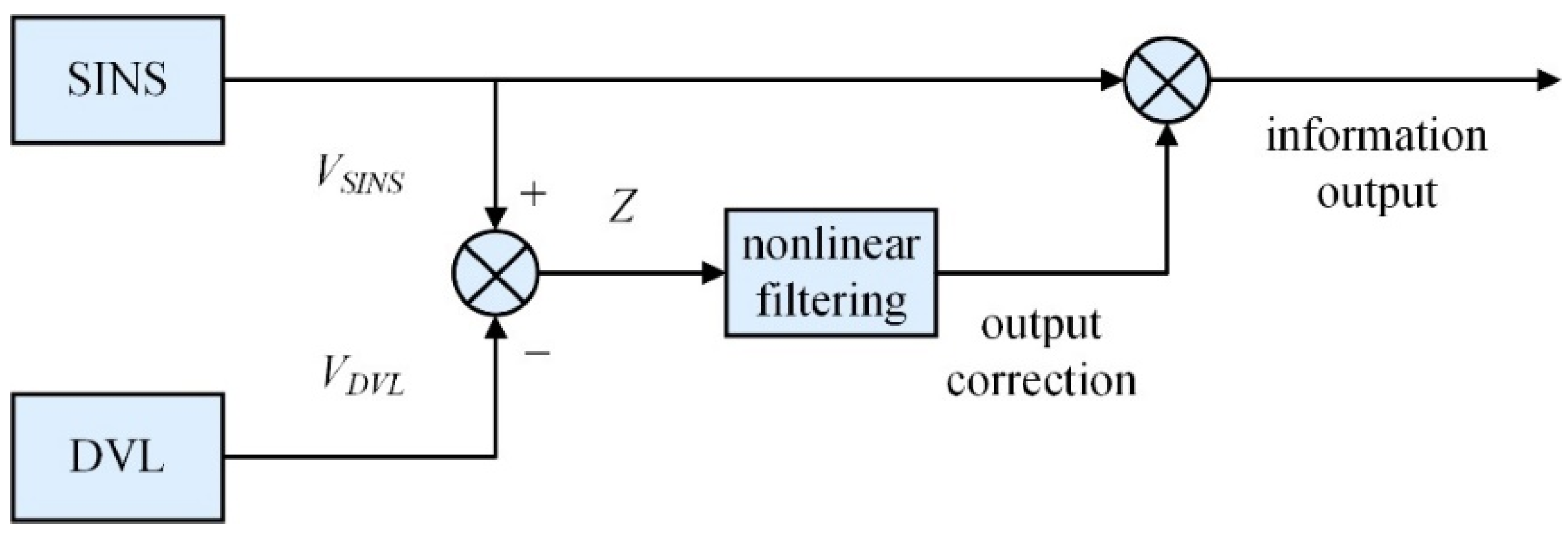
Section 2: Initial alignment of SINS on a dynamic platform: This section describes the error model and state estimation principles used for SINS during their initial alignment on a dynamic platform, with a particular focus on analyzing the nonlinear characteristics of attitude errors under large misalignment angle conditions. By combining velocity information from the Doppler velocity logger (DVL) and the navigation state variables of SINS, the theoretical derivation of the nonlinear error model reveals the core mechanism of error propagation. This lays the theoretical foundation for the subsequent design of the adaptive filtering algorithm based on matrix Lie groups.

Section 3: Optimization design of the AMSSRCKF filtering algorithm based on matrix Lie group representation: This section proposes an adaptive mixed-order spherical simplex-radial cubature Kalman filtering algorithm based on matrix Lie group representation. By mapping attitude errors onto the Lie group manifold space and incorporating exponential and logarithmic mappings, the algorithm avoids linearization errors in rotational motion. The algorithm optimizes the propagation accuracy of state means and covariances using a mixed-order sampling method. Additionally, it dynamically adjusts the noise covariance matrix through innovation sequences, thereby achieving an enhanced filtering accuracy, robustness, and computational efficiency.

Section 4: Particle filter importance density function design and adaptive optimization strategy: This section presents an importance density function design method, based on the MLG-AMSSRCKF algorithm, which significantly enhances the particle distribution’s ability to adapt to non-Gaussian characteristics and higher-order statistical information. A dynamic particle number adjustment mechanism based on Euclidean distance is introduced to effectively reduce redundant particles and optimize the computational efficiency of the algorithm. Additionally, a multidimensional Huber loss function is employed to adaptively optimize particle weights, suppressing the interference of outliers and alleviating the severity of the particle degeneracy problem.

Section 5: Performance analysis: This section provides a comprehensive analysis of the theoretical performance of the MLG-AMSSRCPF algorithm from several aspects, including its sampling strategy, filtering accuracy, computational complexity, adaptability to dynamic environments, and noise resistance. By comparing it with traditional CPF and other improved algorithms, the performance advantages of the MLG-AMSSRCPF algorithm are thoroughly evaluated under conditions of gross measurement error interference, system noise jumps, and strong nonlinearity.

Section 6: Simulation analysis: This section validates the effectiveness of the MLG-AMSSRCPF algorithm through typical simulation scenarios, including cases with no anomalies in measurements or noise, gross measurement error interference, and system noise jumps. The simulation results demonstrate that the algorithm significantly outperforms the traditional cubature particle filter in terms of filtering accuracy, convergence speed, and computational efficiency, exhibiting particularly exceptional performance when dealing with noise jumps and gross measurement error interference.

Section 7: Experimental validation: This section validates the engineering applicability of the MLG-AMSSRCPF algorithm through real-world offshore dynamic platform alignment experiments. The experimental results demonstrate that the algorithm exhibits good adaptability to gross measurement errors and changes in system noise characteristics during initial dynamic platform alignment. Compared to the traditional cubature particle filter algorithm, the heading misalignment angle estimation accuracy of the proposed algorithm is improved by 28.8%, showcasing higher robustness and rapid convergence performance.

Section 8: Conclusions: This section summarizes the main contributions of the MLG-AMSSRCPF algorithm, highlighting its improved high-precision filtering capability, dynamic adaptability, and computational efficiency under complex conditions such as gross measurement error interference and system noise jumps. Combined with simulation and experimental validation, the applicability of the algorithm in complex dynamic environments is analyzed. Finally, this section outlines future research directions, including the optimization of the algorithm’s real-time performance and its potential applications in multi-sensor fusion.

2. Initial Alignment of SINS on a Dynamic Platform

2.1. Working Principle

The initial alignment of a SINS on a moving base can be achieved using the velocity information provided by a Doppler velocity log (DVL) [16]. Under conditions of large heading misalignment angles, the nonlinear characteristics of the error model pose challenges for traditional linear filtering methods, making it difficult to address the problem effectively. Therefore, a nonlinear filtering algorithm is employed in the initial alignment process to enhance both the accuracy and convergence speed of the filtering system. The working principle of this approach is illustrated in Figure 1.

2.2. Error Model of Large Azimuth Misalignment Angle in SINS

Under the condition of large azimuth misalignment angles, the nonlinear error model of a SINS mainly consists of attitude errors and horizontal velocity errors [17].

The transformation matrix between the navigation coordinate system n and the mechanical platform coordinate system $n^{\prime }$ is described by the Euler platform error angle$\varphi ={\left[{\varphi }_x {\varphi }_y {\varphi }_z\right]}^T$, as shown below:

$$C_n^{n^{\prime }}=\left[\begin{array}{ccc}c{\varphi }_{y}c{\varphi }_z-s{\varphi }_{y}s{\varphi }_{x}s{\varphi }_z& c{\varphi }_{y}s{\varphi }_z+s{\varphi }_{y}s{\varphi }_{x}c{\varphi }_z& -s{\varphi }_{y}c{\varphi }_x\\ -c{\varphi }_{x}s{\varphi }_z& c{\varphi }_{x}c{\varphi }_z& s{\varphi }_x\\ s{\varphi }_{y}c{\varphi }_z+c{\varphi }_{y}s{\varphi }_{x}s{\varphi }_z& s{\varphi }_{y}s{\varphi }_z-c{\varphi }_{y}s{\varphi }_{x}c{\varphi }_z& c{\varphi }_{y}c{\varphi }_x\end{array}\right]$$

(1)

In this equation, $s{\varphi }_i$ and $c{\varphi }_i$ represent $\mathrm{s}\mathrm{i}\mathrm{n}\left({\varphi }_i\right)$ and $\mathrm{c}\mathrm{o}\mathrm{s}\left({\varphi }_i\right)$, respectively, where $i=x,y,z$.

Assuming that the angular velocity of the $n^{\prime }$ frame relative to the n frame is ${\omega }_{n{n}^{\prime }}^{n^{\prime }}$, the differential equation for the Euler platform error angles is given as follows:

$$\dot{\varphi }=f^{-1}\left(\varphi \right){\omega }_{n{n}^{\prime }}^{n^{\prime }}$$

(2)

where $f^{-1}\left(\varphi \right)$ is determined as follows:

$$f^{-1}\left(\varphi \right)={\displaystyle \frac{1}{c{\varphi }_x}}\left[\begin{array}{ccc}c{\varphi }_{y}c{\varphi }_x& 0& s{\varphi }_{y}c{\varphi }_x\\ s{\varphi }_{y}s{\varphi }_x& c{\varphi }_x& -c{\varphi }_{y}s{\varphi }_x\\ -s{\varphi }_y& 0& c{\varphi }_y\end{array}\right]$$

(3)

2.2.1. Error Equation

The attitude error equation of the SINS is given as follows:

$$\dot{\varphi }=f^{-1}\left(\varphi \right)\left[\left(I-C_n^{n^{\prime }}\right){\widehat{\omega }}_{in}^n+C_n^{n^{\prime }}\delta {\omega }_{in}^n-C_b^{n^{\prime }}\delta {\omega }_{ib}^b\right]$$

(4)

where ${\widehat{\omega }}_{in}^n$ is the estimated inertial angular velocity in the navigation frame; $\delta {\omega }_{in}^n$ is the inertial angular velocity error in the navigation frame;$\delta {\omega }_{ib}^b$ is the gyroscope measurement error in the body frame; and $C_b^{n^{\prime }}$ is the transformation matrix from the body frame to the mathematical platform frame.

The velocity error equation is written as follows:

$$\begin{array}{ll}& \delta {\dot{\nu }}^n=\left[\mathrm{I}-{\left({\mathrm{C}}_{n^{\prime }}^n\right)}^T\right]{\mathrm{C}}_b^{n^{\prime }}{\widehat{\mathrm{f}}}^b+{\left({\mathrm{C}}_{n^{\prime }}^n\right)}^T{C}_b^{n^{\prime }}\delta {\mathrm{f}}^b\\ & -\left(2\delta {\mathsf{\omega }}_{ie}^n+\delta {\mathsf{\omega }}_{en}^n\right)\times \left({\widehat{\mathsf{\nu }}}^n-\delta {\mathsf{\nu }}^n\right)-\left(2{\widehat{\mathsf{\omega }}}_{ie}^n+{\widehat{\mathsf{\omega }}}_{en}^n\right)\times \delta {\mathsf{\nu }}^n+\delta {\mathrm{g}}^n\end{array}$$

(5)

where $\delta v^n$ is the velocity error in the navigation frame; ${\widehat{f}}^b$ is the specific force estimate in the body frame; $\delta f^b$ is the accelerometer measurement error; $\delta {\omega }_{ie}^n$ is the Earth’s rotational angular velocity error; $\delta {\omega }_{en}^n$ is the vehicle’s motion angular velocity error; ${\widehat{v}}^n$ is the velocity estimate in the navigation frame; and $\delta {\mathrm{g}}^n$ is the gravity error [18]. This study assumes the use of a high-precision gravity field model and neglects the influence of gravity error $\delta {\mathrm{g}}^n$ on the initial alignment.

2.2.2. Filtering Model

In general, the gyro measurement error $\delta {\omega }_{ib}^b$ includes Gaussian white noise $w_g$ with a zero mean and a random constant drift error ${\epsilon }^b$, while the accelerometer measurement error $\delta f^b$ consists of Gaussian white noise $w_a$ with a zero mean and a random constant bias ${\nabla }^b$. Since the horizontal misalignment angle is small and the height error is neglected, the large azimuth misalignment error model of the SINS can be expressed as follows:

(1)

Attitude error equation:

$$\dot{\varphi }=\left(\mathrm{I}-C_n^{n^{\prime }}\right){\widehat{\mathsf{\omega }}}_{in}^n+C_n^{n^{\prime }}\delta {\mathsf{\omega }}_{in}^n-C_b^{n^{\prime }}{\mathsf{\epsilon }}^b+{\mathrm{C}}_b^{n^{\prime }}{w}_g$$

(6)

In this equation, ${\epsilon }^b$ represents the gyro drift error and $w_g$ denotes the gyro white noise.

(2)

Velocity error equation:

$$\delta {\dot{\nu }}^n=\left[\mathrm{I}-{\left({\mathrm{C}}_n^{n^{\prime }}\right)}^{\mathrm{T}}\right]{\mathrm{C}}_b^{n^{\prime }}{\widehat{f}}^b+{\left({\mathrm{C}}_n^{n^{\prime }}\right)}^T{\mathrm{C}}_b^{n^{\prime }}{\nabla }^b-\left(2\delta {\mathsf{\omega }}_{ie}^n+\delta {\mathsf{\omega }}_{en}^n\right)\times {\mathsf{\nu }}^n-\left(2{\mathsf{\omega }}_{ie}^n+{\mathsf{\omega }}_{en}^n\right)\times \delta \mathrm{v}+{\left({\mathrm{C}}_n^{n^{\prime }}\right)}^T{\mathrm{C}}_b^{n^{\prime }}{w}_a$$

(7)

where ${\nabla }^b$ represents the accelerometer bias error and $w_a$ is the accelerometer white noise.

(3)

Gyroscope drift error characteristics:

$${\dot{\epsilon }}_x={\dot{\epsilon }}_y={\dot{\epsilon }}_z=0$$

(8)

(4)

Accelerometer bias characteristics:

$${\dot{\nabla }}_x={\dot{\nabla }}_y={\dot{\nabla }}_z=0$$

(9)

The system state vector is as follows:

$$\mathrm{x}={\left[{\varphi }_x,{\varphi }_y,{\varphi }_z,\delta v_x,\delta v_y,{\epsilon }_x,{\epsilon }_y,{\epsilon }_z,{\nabla }_x,{\nabla }_y\right]}^T$$

(10)

The white noise of the gyroscope and accelerometer is as follows:

$$w={\left[w_{gx},w_{gy},w_{gz},w_{ax},w_{ay},w_{az}\right]}^T$$

(11)

Using the velocity error $z={\left[\delta v_x,\delta v_y\right]}^T$ as the measurement, the system state equation and the measurement equation are as follows:

$$\left\{\begin{array}{l}\dot{x}\left(t\right)=f\left(x\left(t\right),t\right)+G_{w}w\left(t\right)\\ z\left(t\right)=h\left(t\right)x\left(t\right)+v\left(t\right)\end{array}\right.$$

(12)

where $G_w$ is the process noise input matrix, $f\left(x\left(t\right),t\right)$ is the nonlinear vector function, and $h\left(t\right)$ is the measurement matrix, given by $h\left(t\right)=\left[0_{2\times 3}{I}_{2\times 2}{0}_{2\times 5}\right]$. Here, $w\left(t\right)$ represents the process noise and $v\left(t\right)$ represents the measurement noise, both of which follow a Gaussian distribution, i.e.,$v\left(t\right)\sim N\left(0,R\right)$.

3. Optimization Design of the MLG-AMSSRCKF Filtering Algorithm Based on Matrix Lie Group Representation

Building on the classical volume Kalman filtering algorithm, this paper proposes an adaptive mixed-order spherical simplex-radial volume Kalman filtering algorithm based on matrix Lie group representation (MLG-AMSSRCKF). This algorithm integrates the mixed-order spherical simplex-radial volume Kalman filtering (MSSRCKF) method, combining third-order spherical integrals with fifth-order radial integrals, which significantly improves the filtering accuracy of the method while reducing its computational complexity. By utilizing the manifold representation of the Lie group SO(3) [19], the algorithm effectively avoids the errors caused by linearization in representing rotational motion and dynamically adjusts the noise covariance using innovation sequences [20]. This enhances the filter’s adaptability and stability in high-noise environments [21].

The state equation and measurement equation of the nonlinear system are assumed to be as follows:

$$\left\{\begin{array}{l}{x}_k=f\left(x_{k-1}\right)+g\left(x_{k-1}\right)w_{k-1}\\ z_k=h\left(x_k\right)+j\left(x_k\right)v_k\end{array}\right.$$

(13)

In this equation, $f\left(x_{k-1}\right)$ is the state transition function, $h\left(x_k\right)$ is the measurement function, $w_{k-1}$ is the process noise, and $v_k$ is the measurement noise. Both $w_{k-1}$ and ${\mathbf{v}}_k$ are mutually uncorrelated Gaussian white noise processes with a zero mean, and their covariance matrices are $Q$ and $R$, respectively.

The detailed algorithm process is shown in Figure 2.

3.1. Coordinate System Definition

In an inertial navigation system (SINS), several coordinate systems are involved, including the inertial coordinate system (I), the earth coordinate system (E), the navigation coordinate system (n), the mathematical platform coordinate system (n’), and the body coordinate system (b). The navigation coordinate system (n) adopts the east-north-up (ENU) convention, the mathematical platform coordinate system (n’) corresponds to the ideal navigation coordinate system, and the body coordinate system (b) is rigidly connected to the carrier and serves as the reference coordinate system for the SINS’s measurement data.

3.2. Matrix Lie Group and Lie Algebra

To describe the rotation errors of attitude and perform the related calculations, it is necessary to introduce the concepts of the matrix Lie group SO(3) and Lie algebra so(3) [22].

3.2.1. Special Orthogonal Group SO(3)

The special orthogonal group SO(3) is defined as the set of rotation matrices in three-dimensional space:

$$\mathrm{S}\mathrm{O}\left(3\right)=\left\{\mathrm{R}\in {\mathbb{R}}^{3\times 3}\left|{\mathrm{R}}^{\mathrm{T}}\mathrm{R}={\mathrm{I}}_3,\mathrm{d}\mathrm{e}\mathrm{t}\left(\mathrm{R}\right)=1\right\}\right.$$

(14)

where R is a 3 × 3 orthogonal matrix representing a three-dimensional rotation transformation, and $\mathrm{d}\mathrm{e}\mathrm{t}\left(\mathrm{R}\right)$ denotes the determinant of matrix R.

3.2.2. Lie Algebra so(3)

The Lie algebra so(3) of the Lie group SO(3) consists of all 3 × 3 skew-symmetric matrices:

$$so\left(3\right)=\left\{\mathsf{\Omega }\in {\mathbb{R}}^{3\times 3}\mid {\mathsf{\Omega }}^T=-\mathsf{\Omega }\right\}$$

(15)

Each skew-symmetric matrix $\mathsf{\Omega }$ can be represented by a three-dimensional vector $\varphi \in {\mathbb{R}}^3$ as follows:

$$\widehat{\varphi }=\left[\begin{array}{ccc}0& -{\varphi }_z& {\varphi }_y\\ {\varphi }_z& 0& -{\varphi }_x\\ -{\varphi }_y& {\varphi }_x& 0\end{array}\right]$$

(16)

The vector $\varphi ={\left[{\varphi }_x,{\varphi }_y,{\varphi }_z\right]}^{\mathrm{T}}$ represents the rotation vector, and $\widehat{\varphi }$ denotes the skew-symmetric matrix representation of $\varphi$.

3.2.3. Exponential Map and Logarithmic Map

(1)

Exponential Map

The exponential map maps elements of the Lie algebra so(3), represented by the antisymmetric matrix $\widehat{\varphi }$, to elements of the Lie group SO(3), specifically mapping the antisymmetric matrix $\widehat{\varphi }$ to the rotation matrix R:

$$\mathrm{R}=\mathrm{e}\mathrm{x}\mathrm{p}\left(\widehat{\varphi }\right)$$

(17)

Here, exp(⋅) denotes the matrix exponential operation, which is specifically computed using Rodrigues’ rotation formula:

$$R=I_3+{\displaystyle \frac{\mathrm{s}\mathrm{i}\mathrm{n}\left(\parallel \varphi \parallel \right)}{\parallel \varphi \parallel }}\widehat{\varphi }+{\displaystyle \frac{1-\mathrm{c}\mathrm{o}\mathrm{s}\left(\parallel \varphi \parallel \right)}{\parallel \varphi {\parallel }^2}}{\widehat{\varphi }}^2$$

(18)

Here, $\parallel \varphi \parallel$ represents the magnitude of the rotation vector, which indicates the rotation angle, and $\widehat{\varphi }$ is the skew-symmetric matrix form of the rotation vector.

When $\parallel \varphi \parallel$→0, the approximation given by a Taylor expansion a Taylor expansion is given as follows:

$$R\approx I_3+\widehat{\varphi }$$

(19)

(2)

Logarithmic Map

The logarithmic map maps an element R of the Lie group SO(3) to an element $\widehat{\varphi }$ of the Lie algebra so(3), that is, it maps the rotation matrix R to the corresponding skew-symmetric matrix $\widehat{\varphi }$.

$$\widehat{\varphi }=\mathrm{l}\mathrm{o}\mathrm{g}\left(\mathrm{R}\right)$$

(20)

For the rotation matrix R, the logarithmic map is given by the following formula:

$$\widehat{\varphi }={\displaystyle \frac{\theta }{2\mathrm{s}\mathrm{i}\mathrm{n}\left(\theta \right)}}(R-R^T)$$

(21)

where $\theta =\mathrm{a}\mathrm{r}\mathrm{c}\mathrm{c}\mathrm{o}\mathrm{s} \left({\displaystyle \frac{\mathrm{t}\mathrm{r} \left(R\right)-1}{2}}\right)$ and $\mathrm{t}\mathrm{r} \left(R\right)$ represents the trace of the matrix R.

When θ→0, it can be approximated as follows:

$$\widehat{\varphi }\approx {\displaystyle \frac{1}{2}}(R-R^T)$$

(22)

3.3. MSSR Cubature Sampling Rule

To enhance the accuracy of the filtering process and reduce the computational complexity, the MSSR cubature sampling rule integrates third-order spherical integrals and fifth-order radial integrals. The detailed sampling rules are as follows:

Select a set of vectors $a_i={\left[a_{i,1},a_{i,2},\dots ,a_{i,n}\right]}^T$, for $i=1,2,\dots ,n+1$, where n represents the dimension of the state.

$$a_{i,j}=\left\{\begin{array}{ll}-{\left[{\displaystyle \frac{n+1}{n(n-j+2)(n-j+1)}}\right]}^{{\displaystyle \frac{1}{2}}},& j<i\\ {\left[{\displaystyle \frac{(n+1)(n-i+1)}{n(n-i+2)}}\right]}^{{\displaystyle \frac{1}{2}}},& j=i\\ \hspace{1em}\hspace{1em}\hspace{1em}\hspace{1em}0,& j>i\end{array}\right.$$

(23)

The definition of the cubature points ${\xi }_i$ of the filter is as follows:

$$\left\{\begin{array}{l}{\xi }_i=0,\hspace{1em}\hspace{1em}\hspace{1em}\hspace{1em}\hspace{1em}i=0\hfill \\ {\xi }_i={[\sqrt{(n+2)}a]}_i,i=1,2,\cdots ,n+1\hfill \\ {\xi }_i=-{[\sqrt{(n+2)}a]}_i,i=n+2,\cdots ,2n+2\hfill \end{array}\right.$$

(24)

where []i is the set of n-dimensional points calculated using Equation (23), with the number of points being n + 1. The weights corresponding to the cubature points are defined as follows:

$$\left\{\begin{array}{l}{\omega }_i={\displaystyle \frac{2}{n+2}},\hspace{1em}\hspace{1em}\hspace{1em}\hspace{1em}i=0\hfill \\ {\omega }_i={\displaystyle \frac{n}{2(n+1)(n+2)}},i=1,2,\cdots ,2n+2\hfill \end{array}\right.$$

(25)

Based on the aforementioned MSSR cubature sampling rule, the Gaussian summation integral with a mean of 0 and a covariance matrix $\mathrm{I}$ can be expressed as follows:

$$\begin{array}{r}\hfill {\displaystyle {\int }_{R^n}f}(x)\mathrm{N}(x;0,I)\mathrm{d}x={\displaystyle \frac{2}{n+2}}f(0)+{\displaystyle \frac{n}{2(n+1)(n+2)}}\cdot \\ \hfill {\displaystyle \sum _{i=1}^{n+1}\left(f\left(\sqrt{(n+2)}{a}_i\right)+f\left(-\sqrt{(n+2)}{a}_i\right)\right)}\end{array}$$

(26)

For a Gaussian distribution with a mean of $\overline{x}$ and a variance of P, the cubature points are $\sqrt{P}{\xi }_i+\overline{x}$. Thus, the multidimensional integral can be expressed as follows:

$$\begin{array}{l}{\displaystyle {\int }_{R^n}f}(x)N(x;\overline{x},P)\mathrm{d}x={\displaystyle \frac{2}{n+2}}f(\overline{x})+{\displaystyle \frac{n}{2(n+1)(n+2)}}.\\ \begin{array}{cccc}& & & \end{array}{\displaystyle \sum _{i=1}^{n+1}\left(f\left(\sqrt{(n+2)P}{a}_i+\overline{x}\right)+f\left(-\sqrt{(n+2)P}{a}_i+\overline{x}\right)\right)}\end{array}$$

(27)

where $P=\sqrt{P}\cdot (\sqrt{P}{)}^T$.

3.4. Matrix Lie Group-Based AMSSRCKF Filtering Algorithm

This paper presents an adaptive mixed-order spherical simplex-radial volume sampling-based constrained Kalman filter algorithm (MLG-AMSSRCKF) based on matrix Lie group representation. The algorithm represents the attitude errors as elements of the Lie group SO(3), thereby avoiding the linearization issue of rotational errors and enabling accurate state estimation within the Lie group manifold space. Meanwhile, velocity errors, as well as errors from gyroscopes and accelerometers, are still represented in the traditional Euclidean space. To improve the algorithm’s filtering accuracy, a mixed-order spherical simplex-radial volume sampling rule is utilized, which generates volume points on the Lie group manifold. By combining exponential and logarithmic mappings, the algorithm effectively handles attitude errors and optimizes the filter’s convergence speed and computational efficiency. Furthermore, through an adaptive noise adjustment mechanism, the algorithm achieves high precision and robustness in state estimation under complex dynamic environments. The specific steps of the algorithm are as follows.

3.4.1. Initialization

State mean:

$$X_0=(\delta {\varphi }_0,\delta v_0^n,{\epsilon }_0,{\nabla }_0)$$

(28)

where $\delta {\varphi }_0\in SO\left(3\right)$ represents the initial attitude error, expressed in rotation matrix form; $\delta v_0^n\in {\mathbb{R}}^2$ is the initial horizontal velocity error in the navigation frame; ${\epsilon }_0\in {\mathbb{R}}^3$ represents the initial gyroscope drift error estimate; and ${\nabla }_0\in {\mathbb{R}}^2$ denotes the initial accelerometer horizontal bias error estimate.

State dimension and state vector:

The state dimension is n = 10, and the corresponding state vector is given by:

$$x=[\delta {\varphi }_x,\delta {\varphi }_y,\delta {\varphi }_z,\delta v_x^n,\delta v_y^n,{\epsilon }_x,{\epsilon }_y,{\epsilon }_z,{\nabla }_x,{\nabla }_y{]}^T$$

(29)

Covariance matrix:

$$P_0=\left[\begin{array}{cccc}{P}_{\delta \varphi ,0}& 0& 0& 0\\ 0& P_{{\delta }_{v,0}}& 0& 0\\ 0& 0& P_{\epsilon ,0}& 0\\ 0& 0& 0& P_{\nabla ,0}\end{array}\right]$$

(30)

where $P_{\delta \varphi ,0}\in {\mathbb{R}}^{3\times 3}$ is the covariance matrix of the attitude error, defined in the Lie algebra so(3); $P_{\delta v,0}\in {\mathbb{R}}^{2\times 2}$ is the covariance matrix of the horizontal velocity error; $P_{\epsilon ,0}\in {\mathbb{R}}^{3\times 3}$ is the covariance matrix of the gyroscope drift error; and $P_{\nabla ,0}\in {\mathbb{R}}^{2\times 2}$ is the covariance matrix of the accelerometer horizontal bias error.

3.4.2. Time Update

Step 1: Compute the square root of the covariance

The square root matrix ${\mathrm{S}}_k$ of the covariance matrix ${\mathrm{P}}_k$ is computed using the Cholesky decomposition:

$${\mathrm{P}}_k={\mathrm{S}}_k{\mathrm{S}}_k^{\mathrm{T}}$$

(31)

where $S_k$ is the lower triangular matrix.

Step 2: Generate cubature sampling points

Cubature point deviations:

$${\xi }_i=\sqrt{n+2}{S}_k{a}_i,i=\mathrm{0,1},2,\dots ,2n+2$$

(32)

where the state dimension is n = 10, and $a_i$ is the direction vector generated by the MSSR rule.

Constructing the cubature points:

For each cubature point $i$, the corresponding state variable is calculated based on the deviation vector ${\xi }_i$:

(1)

Attitude error:

The attitude error matrix corresponding to the $\mathrm{i}$-th cubature point is calculated, and the deviation is mapped to SO(3) using the exponential map:

$${\delta \varphi }_k^{\left(i\right)}={\delta \varphi }_k\mathrm{e}\mathrm{x}\mathrm{p}\left({\left(\delta {\varphi }_i\right)}^{\wedge }\right)$$

(33)

where ${\delta \varphi }_k$ represents the attitude error mean, expressed as a rotation matrix. ${\left(\delta {\varphi }_i\right)}^{\wedge }$ is the skew-symmetric matrix of$\delta {\varphi }_i$, and ${\delta \varphi }_k^{\left(i\right)}$ represents the attitude error matrix corresponding to the $i$-th cubature point.$\delta {\varphi }_i$ is the cubature sampling deviation of the attitude error mean, which is determined by extracting the first three elements of ${\xi }_i$.

(2)

Horizontal velocity error:

The horizontal velocity error corresponding to the $i$-th cubature point is calculated as follows:

$$\delta v_k^{n\left(i\right)}=\delta v_k^n+\delta \left(\delta v_i^n\right)$$

(34)

where $\delta v_k^n$ represents the mean horizontal velocity error and $\delta \left(\delta v_i^n\right)$ is the cubature sampling deviation from this mean, which is determined by extracting the fourth and fifth elements of ${\xi }_i$.

(3)

Gyroscope drift error:

The gyroscope drift error corresponding to the $i$-th cubature point is calculated as follows:

$${\epsilon }_k^{\left(i\right)}={\epsilon }_k+\delta {\epsilon }_i$$

(35)

where ${\epsilon }_k$ represents the mean of the gyroscope drift error, and $\delta {\epsilon }_i$ denotes the cubature sampling deviation of the drift error, which is determined by extracting the sixth, seventh, and eighth elements of ${\xi }_i$.

(4)

Accelerometer bias error:

The accelerometer bias error corresponding to the $i$-th cubature point is calculated as follows:

$${\nabla }_k^{\left(i\right)}={\nabla }_k+\delta {\nabla }_i$$

(36)

where ${\nabla }_k$ represents the mean accelerometer bias error; $\delta {\nabla }_i$ is the cubature sampling deviation from the mean, which is determined by extracting the 9th and 10th elements of ${\xi }_i$.

Step 3: Time propagation of the cubature points

(1)

Update of the Attitude Error:

Definition:

$$\delta {\omega }_{\mathrm{e}\mathrm{f}\mathrm{f}}^{\left(i\right)}=(I-C_n^{\left(n^{\prime }\right)}){\widehat{\omega }}_{in}^n+C_n^{\left(n^{\prime }\right)}\delta {\omega }_{in}^n-C_b^{\left(n^{\prime }\right)}{\epsilon }_k^{\left(i\right)}+C_b^{\left(n^{\prime }\right)}{w}_{g,k}$$

(37)

The attitude error update formula is as follows:

$$\delta {\varphi }_{k+1}^{\left(i\right)}={\delta \varphi }_k^{\left(i\right)}\cdot \mathrm{e}\mathrm{x}\mathrm{p} \left({\left(\delta {\omega }_{\mathrm{e}\mathrm{f}\mathrm{f}}^{\left(i\right)}\right)}^{\wedge }\mathsf{\Delta }t\right)$$

(38)

The total angular velocity error of the $\mathit{i}$-th cubature sampling point is denoted as $\delta {\omega }_{\mathrm{e}\mathrm{f}\mathrm{f}}^{\left(i\right)}$, where ${\omega }_{in}^n$ is the inertial angular velocity in the navigation frame,$w_{g,k}$ represents the white noise from the gyroscope, and $\Delta t$ is the sampling time interval.

(2)

Update of Horizontal Velocity Error:

Definition:

$$\delta a_{\mathrm{e}\mathrm{f}\mathrm{f}}^{n\left(i\right)}=\left[I-(C_n^{\left(n^{\prime }\right)}{)}^{\mathrm{T}}\right]C_b^{\left(n^{\prime }\right)}{\widehat{f}}^b+(C_n^{\left(n^{\prime }\right)}{)}^{\mathrm{T}}{C}_b^{\left(n^{\prime }\right)}\left({\nabla }_k^{\left(i\right)}+w_{a,k}\right)-(2\delta {\omega }_{ie}^n+\delta {\omega }_{en}^n)\times v^n-(2{\omega }_{ie}^n+{\omega }_{en}^n)\times \delta v_k^{n\left(i\right)}+\delta g^n$$

(39)

The update formula for the horizontal velocity error is as follows:

$$\delta v_{k+1}^{n\left(i\right)}=\delta v_k^{n\left(i\right)}+\delta a_{\mathrm{e}\mathrm{f}\mathrm{f}}^{n\left(i\right)}\mathsf{\Delta }t$$

(40)

where $\delta a_{\mathrm{e}\mathrm{f}\mathrm{f}}^{n\left(i\right)}$ represents the total acceleration error at the $\mathit{i}$-th cubature sample point, and $w_{a,k}$ is the accelerometer white noise.

(3)

Update of Gyroscope Drift Error:

Since the gyroscope drift error is assumed to be constant, the update is given by the following:

$${\epsilon }_{k+1}^{\left(i\right)}={\epsilon }_k^{\left(i\right)}$$

(41)

(4)

Update of Accelerometer Zero-Bias Error:

Since the accelerometer’s zero-bias error is assumed to be constant, the update is given by the following:

$${\nabla }_{k+1}^{\left(i\right)}={\nabla }_k^{\left(i\right)}$$

(42)

Step 4: Calculation of predicted state mean

Directly applying a linear weighted average to the attitude matrix is not applicable in the SO(3) space for predicting the state mean, as it may introduce biases. Therefore, this algorithm adopts a weighted least squares method. By using the logarithmic map, the distances between rotation matrices are transformed into the magnitudes of rotation vectors in the Lie algebra space. After minimizing the weighted rotation error, the result is mapped back to the SO(3) space via the exponential map, ensuring accuracy and geometric consistency. This approach is more stable under nonlinear conditions and is suitable for meeting the initial alignment requirements of large attitude misalignment angles.

(1)

Attitude Mean:

The rotation matrix $\delta \varphi$ is sought as the optimization variable in SO(3). Let the objective function be the following:

$$J(\delta \varphi )=\sum _{i=0}^{2n+2} w_i{∥{\left(\log \left(\delta {\varphi }^{-1}\delta {\varphi }_{k+1}^{\left(i\right)}\right)\right)}^{\vee }∥}^2$$

This is a function of $\delta \varphi$, representing the sum of squared weighted rotation errors. The optimal solution $\delta {\varphi }_{k+1}$ is as follows:

$$\delta {\varphi }_{k+1}=\mathrm{a}\mathrm{r}\mathrm{g} \underset{\delta \varphi \in SO\left(3\right)}{min} J(\delta \varphi )$$

(43)

The objective is to find a value of $\delta \varphi$ that minimizes the objective function $J\left(\delta \varphi \right)$, where the optimal solution $\delta {\varphi }_{k+1}$ represents the attitude error mean at time k + 1.

Here, $\delta \varphi \in$ SO(3) is the optimization variable, representing the attitude error mean to be solved; $\delta {\varphi }_{k+1}$ is the solution to the optimization problem, i.e., the attitude error mean at time k + 1, which is obtained by solving the above optimization problem; $\delta {\varphi }_{k+1}^{\left(i\right)}\in$ SO(3) is the attitude error matrix corresponding to the $i$-th cubature point; $w_i$ is the weight of the $i$-th cubature point; $(\delta \varphi {)}^{-1}\delta {\varphi }_{k+1}^{\left(i\right)}\in$ SO(3) is the relative rotation matrix from $\delta \varphi$ to $\delta {\varphi }_{k+1}^{\left(i\right)}$; $\log \left((\delta \varphi {)}^{-1}\delta {\varphi }_{k+1}^{\left(i\right)}\right)\in$ so(3) is the logarithmic map from the Lie group to the Lie algebra, which allows the mapping of the relative rotation matrix to the Lie algebra so(3);$(\cdot {)}^{\vee }\in {\mathbb{R}}^3$ is the vectorization operation, which maps the skew-symmetric matrix in the Lie algebra to a three-dimensional vector in Euclidean space; ${∥\cdot ∥}^2$ is the square of the L2 norm of the vector, representing the square of the magnitude of the rotation vector, i.e., the square of the rotation angle [23].

(2)

Other State Means:

Horizontal velocity error mean:

$$\delta v_{k+1}^n={\sum }_{i=0}^{2n+2}{w}_i \delta v_{k+1}^{n\left(i\right)}$$

(44)

Gyroscope drift error mean:

$${\epsilon }_{k+1}={\sum }_{i=0}^{2n+2}{w}_i {\epsilon }_{k+1}^{\left(i\right)}$$

(45)

Accelerometer bias error mean:

$${\nabla }_{k+1}={\sum }_{i=0}^{2n+2}{w}_i {\nabla }_{k+1}^{\left(i\right)}$$

(46)

Step 5: Calculation of predicted covariance

(1)

State error calculation:

For each cubature point $i$, calculate the state error:

$$\delta {\xi }_{k+1}^{\left(i\right)}=\left[\begin{array}{c}{\left(\log \left((\delta {\varphi }_{k+1}{)}^{-1}\delta {\varphi }_{k+1}^{\left(i\right)}\right)\right)}^{\vee }\\ \delta v_{k+1}^{n\left(i\right)}-\delta v_{k+1}^n\\ {\epsilon }_{k+1}^{\left(i\right)}-{\epsilon }_{k+1}\\ {\nabla }_{k+1}^{\left(i\right)}-{\nabla }_{k+1}\end{array}\right]$$

(47)

(2)

Calculation of the Predicted Covariance Matrix:

$$P_{k+1}^{-}=\sum _{i=0}^{2n+2}{w}_i \delta {\xi }_{k+1}^{\left(i\right)}{\left(\delta {\xi }_{k+1}^{\left(i\right)}\right)}^{\mathrm{T}}+Q_k$$

(48)

where $Q_k$ is the process noise covariance matrix.

3.4.3. Measurement Update

The filter uses error state representation and employs error forms in its measurement equations.

Step 1: Generate measurement cubature points

For each state error cubature point $\delta {\xi }_{k+1}^{\left(i\right)}$, calculate the corresponding measurement error cubature point:

$$\delta z_{k+1}^{\left(i\right)}=H\delta {\xi }_{k+1}^{\left(i\right)}$$

(49)

Step 2: Calculate the predicted measurement error mean

Since the predicted mean of the error state is zero, the following equation can be used:

$$\delta z_{k+1}^{\mathrm{pred}}=E\left[\delta z_{k+1}\right]=HE\left[\delta {\xi }_{k+1}\right]=0$$

(50)

Step 3: Calculate the measurement covariance and cross-covariance

(1)

Measurement Covariance:

$$P_{zz}={\sum }_{i=0}^{2n+2}{w}_i \delta z_{k+1}^{\left(i\right)}{\left(\begin{array}{c}\delta z_{k+1}^{\left(i\right)}\end{array}\right)}^{\mathrm{T}}+R_k$$

(51)

(2)

Cross-Covariance:

$$P_{xz}={\sum }_{i=0}^{2n+2}{w}_i \delta {\xi }_{k+1}^{\left(i\right)}{\left(\delta z_{k+1}^{\left(i\right)}\right)}^T$$

(52)

Step 4: Calculate the Kalman gain

$${\mathrm{K}}_{k+1}={\mathrm{P}}_{xz}{\mathrm{P}}_{zz}^{-1}$$

(53)

Step 5: Update the state estimation

(1)

Calculate the state increment:

$$\delta {\xi }_{k+1}=K_{k+1}\left(\begin{array}{c}{z}_{k+1}^{\mathrm{o}\mathrm{b}\mathrm{s}}-H{\widehat{x}}_{k+1}^{-}\end{array}\right)$$

(54)

where $z_{k+1}^{\mathrm{o}\mathrm{b}\mathrm{s}}$ is the observed measurement, and ${\widehat{x}}_{k+1}^{-}$ is the prior state estimate. $\delta {\xi }_{k+1}$ includes the following components:

$$\delta {\xi }_{k+1}=\left[\begin{array}{c}\delta {\varphi }_{k+1}\\ \delta v_{k+1}^n\\ \delta {\epsilon }_{k+1}\\ \delta {\nabla }_{k+1}\end{array}\right]$$

(2)

Update state:

Attitude error update:

$$\delta {\varphi }_{k+1}^{+}=\delta {\varphi }_{k+1}^{-}\cdot \mathrm{e}\mathrm{x}\mathrm{p}\left({\left(\delta {\varphi }_{k+1}\right)}^{\wedge }\right)$$

(55)

where $\delta {\varphi }_{k+1}^{-}$ is the prior attitude error,$\delta {\varphi }_{k+1}$ is the attitude error increment corresponding to the state increment $\delta {\xi }_{k+1}$, and $\delta {\varphi }_{k+1}^{+}$ is the updated posterior attitude error.

Horizontal velocity error update:

$$\delta v_{k+1}^{n+}=\delta v_{k+1}^{n-}+\delta v_{k+1}^n$$

(56)

where $\delta v_{k+1}^{n-}$ is the prior horizontal velocity error, $\delta v_{k+1}^n$ is the horizontal velocity error increment corresponding to the state increment $\delta {\xi }_{k+1}$, and $\delta v_{k+1}^{n+}$ is the updated posterior horizontal velocity error.

Gyroscope drift error update:

$${\epsilon }_{k+1}^{+}={\epsilon }_{k+1}^{-}+\delta {\epsilon }_{k+1}$$

(57)

where ${\epsilon }_{k+1}^{-}$ is the prior gyroscope drift error, $\delta {\epsilon }_{k+1}$ is the gyroscope drift error increment corresponding to the state increment $\delta {\xi }_{k+1}$, and ${\epsilon }_{k+1}^{+}$ is the updated posterior gyroscope drift error.

Accelerometer bias error update:

$${\nabla }_{k+1}^{+}={\nabla }_{k+1}^{-}+\delta {\nabla }_{k+1}$$

(58)

where ${\nabla }_{k+1}^{-}$ is the prior accelerometer bias error, $\delta {\nabla }_{k+1}$ is the accelerometer bias error increment corresponding to the state increment $\delta {\xi }_{k+1}$, and ${\nabla }_{k+1}^{+}$ is the updated posterior accelerometer bias error.

Step 6: Update of the covariance matrix

$$P_{k+1}^{+}=P_{k+1}^{-}-K_{k+1}{P}_{zz}{K}_{k+1}^T$$

(59)

3.4.4. Adaptive Noise Adjustment

To improve the filter’s adaptability in complex noise environments, an adaptive noise covariance update mechanism is employed to dynamically adjust the process noise covariance $Q_k$ and the measurement noise covariance $R_k$ [24]. The specific steps are as follows:

Step 7: Adjust process noise covariance $Q_k$

(1)

Calculate the state residual:

Prior error state estimation:

$$\delta {\xi }_{k+1}^{-}=0$$

Posterior error state estimation:

$$\delta {\xi }_{k+1}^{+}=K_{k+1}\left(\begin{array}{c}{z}_{k+1}^{\mathrm{o}\mathrm{b}\mathrm{s}}-H{\widehat{x}}_{k+1}^{-}\end{array}\right)$$

(60)

State residual:

$$\delta {\xi }_{k+1}^{\mathrm{res}}=\delta {\xi }_{k+1}^{+}-\delta {\xi }_{k+1}^{-}=\delta {\xi }_{k+1}^{+}$$

(61)

where $\delta {\xi }_{k+1}^{+}$ is the posterior state estimation error, $K_{k+1}$ is the filter gain, $z_{k+1}^{\mathrm{obs}}$ is the measurement, $H$ is the measurement matrix, and ${\widehat{x}}_{k+1}^{-}$ is the prior state estimate.

(2)

Update the process noise covariance:

$$Q_{k+1}=\gamma Q_k+\left(1-\gamma \right)\left(\delta {\xi }_{k+1}^{\mathrm{r}\mathrm{e}\mathrm{s}}{\left(\delta {\xi }_{k+1}^{\mathrm{r}\mathrm{e}\mathrm{s}}\right)}^{\mathrm{T}}+K_{k+1}{R}_k{K}_{k+1}^{\mathrm{T}}\right)$$

(62)

where $\gamma$ is the forgetting factor, with a value range of 0 < $\gamma$ < 1.

Step 8: Adjusting the measurement noise covariance ${\mathrm{R}}_{\mathrm{k}}$

(1)

Calculate the measurement innovation covariance estimate:

Measurement residual:

$$\delta z_{k+1}=z_{k+1}^{\mathrm{o}\mathrm{b}\mathrm{s}}-H{\widehat{x}}_{k+1}^{-}$$

Measurement innovation covariance estimate:

$$S_z=\delta z_{k+1}\delta z_{k+1}^T$$

$$S_z=\left(\begin{array}{c}{z}_{k+1}^{\mathrm{o}\mathrm{b}\mathrm{s}}-H{\widehat{x}}_{k+1}^{-}\end{array}\right){\left(\begin{array}{c}{z}_{k+1}^{\mathrm{o}\mathrm{b}\mathrm{s}}-H{\widehat{x}}_{k+1}^{-}\end{array}\right)}^{\mathrm{T}}$$

(63)

(2)

Update the measurement noise covariance:

$$R_{k+1}=\lambda R_k+\left(1-\lambda \right)\left(\begin{array}{c}{S}_z-H{P}_{k+1}^{-}{H}^{\mathrm{T}}\end{array}\right)$$

(64)

where λ is the forgetting factor, with a range of 0 < λ < 1, and $P_{k+1}^{-}$ is the prior state covariance matrix.

Step 9: Ensuring the positive definiteness of the covariance matrix

A positive definiteness check is performed on the updated $Q_{k+1}$ and $R_{k+1}$. If non-positive definiteness is detected (e.g., negative eigenvalues), the matrices can be adjusted or positive-definiteness constraints can be applied to correct them, ensuring the stability of the filtering process and the reliability of the computation.

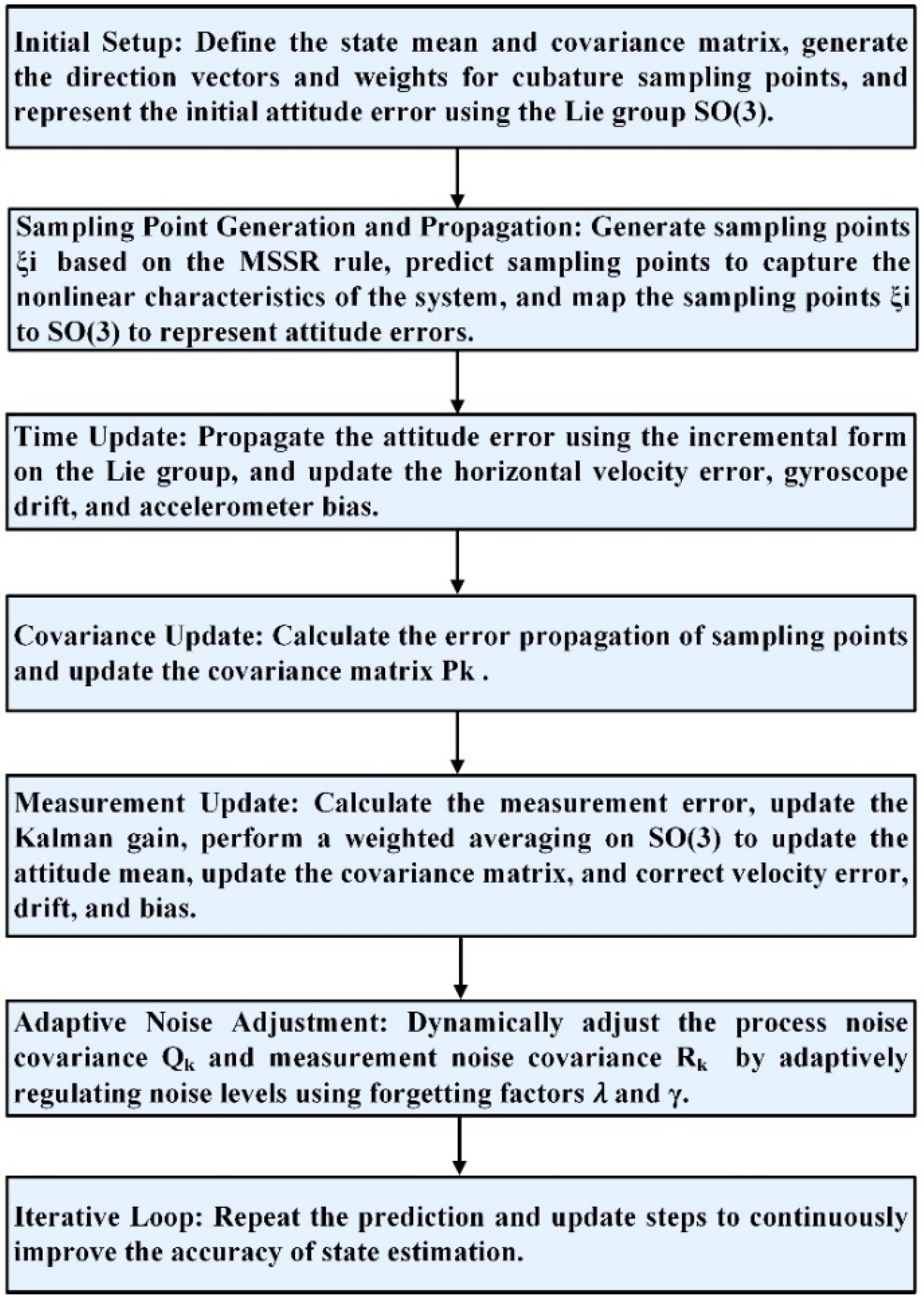
4. Design of Importance Density Function and Adaptive Optimization Strategy for Particle Filtering

The performance of particle filtering methods largely depends on the choice of the importance density function. A well-designed importance density function can not only effectively mitigate particle degeneracy but also significantly improve both the accuracy and computational efficiency of the filtering process. To address this critical issue, this paper proposes an adaptive mixed-order spherical simplex-radial volume particle filtering algorithm based on matrix Lie group representation (MLG-AMSSRCPF), aiming to achieve efficient and precise state estimation in complex environments.

This algorithm combines mixed-order spherical simplex-radial volume Cubature Kalman filtering (MSSRCKF) with matrix Lie group representation, and integrates an adaptive noise covariance update mechanism [25]. By optimizing the mean and variance of the state, a more accurate importance density function for particle filtering is designed, ensuring that the generated particle set can more effectively handle complex state variations and thus improving the filter’s performance.

Furthermore, the MLG-AMSSRCPF algorithm uses Euclidean distance to measure the similarity between particles and dynamically adjusts the number of particles to reduce the computational complexity while maintaining accuracy. At the same time, an adaptive multidimensional Huber loss function is employed to adjust particle weights, suppressing the influence of outliers on the filtering results and thereby significantly enhancing the robustness of the algorithm [26].

The comprehensive application of these optimization strategies strengthens the filter’s performance in dynamic noise environments, ensuring its efficiency and reliability in high-dimensional and real-time applications. The workflow of the MLG-AMSSRCPF algorithm is shown in Figure 3.

The specific workflow of the MLG-AMSSRCPF algorithm is as follows:

(1)

Initialization

Particle state initialization:

$$x_0^i\sim p\left(x_0\right), w_0^i={\displaystyle \frac{1}{N}}$$

(65)

where N is the initial number of particles, $x_0^i$ is the initial state of the i-th particle, and $w_0^i$ is the initial weight.

Mean and covariance matrix initialization:

$${\widehat{x}}_0^i=E\left[x_0^i\right], P_0^i=E\left[\left(x_0^i-{\widehat{x}}_0^i\right){\left(x_0^i-{\widehat{x}}_0^i\right)}^T\right]$$

(66)

where ${\widehat{x}}_0^i$ is the expected value of the initial state and $P_0^i$ is the initial covariance matrix.

Parameter settings: set $\gamma ,\alpha ,\delta ,N_{\mathrm{m}\mathrm{a}\mathrm{x}},\mathrm{a}\mathrm{n}\mathrm{d} N_{\mathrm{m}\mathrm{i}\mathrm{n}}$, where $\gamma$ is the Euclidean distance threshold used to assess the similarity between particles; $\alpha$ is the cost function threshold used to control particle number adjustments; $\delta$ is the parameter of the Huber loss function, which is used to control the filter’s sensitivity to large residuals; and $N_{\mathrm{m}\mathrm{a}\mathrm{x}}$ and $N_{\mathrm{m}\mathrm{i}\mathrm{n}}$ are the upper and lower limits of the particle numbers, and ensure the efficiency and accuracy of the algorithm.

(2)

State Prediction

Particle prediction: predict the particles using the system state transition equation, in which the particles generate the next state based on the current state and the importance density function:

$$x_k^i\sim q\left(x_k^i\mid x_{k-1}^i,z_k\right)$$

(67)

where $q\left(x_k^i\mid x_{k-1}^i,z_k\right)$ is the importance density function optimized by the MLG-AMSSRCKF algorithm.

Importance density function design:

The importance density function is designed using the MLG-AMSSRCKF:

$$\left[{\widehat{x}}_k^i,P_k^i\right]=\mathrm{M}\mathrm{L}\mathrm{G}-\mathrm{A}\mathrm{M}\mathrm{S}\mathrm{S}\mathrm{R}\mathrm{C}\mathrm{K}\mathrm{F}\left[{\widehat{x}}_{k-1}^i,P_{k-1}^i,z_k\right]$$

(68)

Generate particles based on the new distribution:

$$x_k^i\sim N\left({\widehat{x}}_k^i,P_k^i\right)$$

(69)

(3)

Particle Elimination and Selection

To avoid particle degradation caused by particles being too similar, an elimination strategy based on Euclidean distance is used to reduce the number of particles while retaining representative ones.

Euclidean distance judgment:

Use the Euclidean distance $∥x_{d,k}^{\left(i\right)}-x_{d,k}^{\left(i+1\right)}∥$ between neighboring particles to judge similar particles:

$$∥x_{d,k}^{\left(i\right)}-x_{d,k}^{\left(i+1\right)}∥<\gamma$$

(70)

where γ is the preset Euclidean distance threshold that is used to measure the similarity between two particles in state space. After sorting, Euclidean distances are computed only between adjacent particles, resulting in a computational complexity of O(N⋅ d). Given that the number of particles (≤200) and the state dimension (≤15) are both constrained, the overall computational cost remains manageable. This evaluation is performed only once during the sampling stage, exerting minimal impact on real-time performance.

Particle selection:

If $∥x_{d,k}^{\left(i\right)}-x_{d,k}^{\left(i+1\right)}∥<\gamma$, select based on the particle weights;

If $w_k^{\left(i\right)}>w_k^{\left(i+1\right)}$, retain the i-th particle $x_{d,k}^{\left(i\right)}$;

Otherwise, retain the i+1-th particle $x_{d,k}^{\left(i+1\right)}$;

If the condition is not met, retain both particles.

Update particle set:

The retained particles form the set $S_t$, while the eliminated particles form the set $K_t$.

(4)

Adaptive Particle Number Adjustment

Through the previous steps, the elimination of particles was achieved to reduce the computational cost. However, excessive reduction in the number of particles may lead to a loss of particle diversity, which could cause filter divergence. Therefore, a cost function can be introduced to dynamically adjust the number of particles by calculating the innovation error cost function ${\mathit{\xi }}^{\mathit{k}}\left(\mathit{n}\right)$. Specifically, a threshold $\alpha$ is predefined, and by comparing the current cost function value with the threshold, it is determined whether to decrease or increase the number of particles.

Innovation error cost function:

$${\xi }_k^2\left(n\right)={\left(z_k-h_k\left({\widehat{x}}_k\right)\right)}^T{R}_k^{-1}\left(z_k-h_k\left({\widehat{x}}_k\right)\right)$$

(71)

where ${\mathit{z}}_{\mathit{k}}$ is the observation, $R_k$ is the observation noise covariance matrix, ${\widehat{\mathit{x}}}_{\mathit{k}}$ is the state estimate obtained using the particles retained in the set $S_t$ and their corresponding weights, and $n$ is the number of particles.

Particle number adjustment strategy:

If ${\xi }_k\left(n\right)<\alpha$, it indicates that the number of particles is sufficient, and the particle number can be reduced:

$$N_{k+1}=\mathrm{a}\mathrm{r}\mathrm{g}{\mathrm{m}\mathrm{i}\mathrm{n}}_{n\in \left[N_{\mathrm{m}\mathrm{i}\mathrm{n}},N_{\mathrm{m}\mathrm{a}\mathrm{x}}\right]}{\xi }_k\left(n\right)$$

(72)

If ${\xi }_k\left(n\right)>\alpha$, it indicates that more particles are needed to maintain filtering accuracy:

$$N_{k+1}\in \left[N_k,N_{\mathrm{m}\mathrm{a}\mathrm{x}}\right]$$

(73)

This process ensures the dynamic adjustment of the number of particles, avoiding the computational burden of an excessive number of particles while maintaining filtering accuracy.

(5)

Weight Calculation and Adjustment

To enhance the robustness of the algorithm against outlier observations, a multidimensional Huber loss function is introduced for adaptive weight adjustment.

Weight calculation:

$$w_k^i={\displaystyle \frac{p\left(z_k\mid x_k^i\right)P\left(x_k^i\mid x_{k-1}^i\right)}{q\left(x_k^i\mid x_{k-1}^i,z_k\right)}}$$

(74)

Observation residual calculation:

$$r_i=z_k-h\left(x_k^i\right)$$

(75)

Multidimensional Huber loss function for weight adjustment:

To handle multidimensional observation residuals, the multidimensional Huber loss function is introduced for weight adjustment:

$${\gamma }_i=\left\{\begin{array}{ll}1,& \parallel {\mathrm{r}}_i\parallel \le \delta \\ {\displaystyle \frac{\delta }{\parallel {\mathrm{r}}_i\parallel }},& \parallel {\mathrm{r}}_i\parallel >\delta \end{array}\right.$$

(76)

where $\parallel {\mathbf{r}}_i\parallel$ represents the multidimensional norm of the observation residual, which is calculated using the Mahalanobis distance:

$$\parallel {\mathrm{r}}_i\parallel =\sqrt{{\mathrm{r}}_i^T{\mathrm{R}}^{-1}{\mathrm{r}}_i}$$

(77)

Here, R denotes the covariance matrix of the observation noise, which characterizes the variability of noise across different observation dimensions. Incorporating this weighting matrix into the Mahalanobis distance enhances the ability to distinguish abnormal observations. The parameter $\delta$ is a tuning factor in the Huber loss function, used to control the sensitivity to large observation residuals, thereby enabling the filter to smooth small errors while suppressing the influence of outliers on the estimation results.

Updated particle weights:

$$w_k^i=w_k^i\cdot {\gamma }_i$$

(78)

(6)

Particle Weight Normalization:

Weight normalization:

$$w_k^i={\displaystyle \frac{w_k^i}{\sum _{j=1}^N{w}_k^j}}$$

(79)

(7)

Resampling:

Resample based on the normalized particle weights:

$${\left\{x_k^j,w_k^j\right\}}_{j=1}^N=\mathrm{R}\mathrm{e}\mathrm{s}\mathrm{a}\mathrm{m}\mathrm{p}\mathrm{l}\mathrm{e}\left({\left\{x_k^i,w_k^i\right\}}_{i=1}^N\right)$$

(80)

(8)

State Estimation and Covariance Calculation:

$${\widehat{x}}_k={\sum }_{i=1}^N{w}_k^i{x}_k^i$$

(81)

$$P_k={\sum }_{i=1}^N{w}_k^i\left(x_k^i-{\widehat{x}}_k\right){\left(x_k^i-{\widehat{x}}_k\right)}^T$$

(82)

(9)

Iteration:

Set $k=k+1$, and repeat steps 2 through 8 until the filtering process is complete.

In the MLG-AMSSRCPF algorithm, the use of Euclidean distance and the design of the multidimensional Huber loss function are based on their unique advantages in high-dimensional nonlinear filtering.

Firstly, Euclidean distance is known for its simplicity and intuitiveness in calculation. By quickly computing the state-space distances between particles, it can effectively identify particle similarities and prevent particle degeneracy, especially in high-dimensional state estimation. In the MLG-AMSSRCPF algorithm, the particle count is set between 100 and 200, with a dynamic adjustment mechanism being used to balance the filtering accuracy and computational complexity. References [27,28] indicate that, for high-dimensional nonlinear problems in tightly coupled SINS/GPS navigation, setting the particle count to 100–200 effectively reduces the computational burden while maintaining sufficient filtering accuracy and particle diversity. By setting a Euclidean distance threshold of γ = 0.5, the algorithm can effectively identify and avoid high similarities between particles, preventing particle degeneracy. References [29,30] have conducted in-depth studies demonstrating the effectiveness of this strategy in solving multidimensional nonlinear navigation problems. Furthermore, the MLG-AMSSRCPF algorithm introduces a cost function threshold of α = 0.3 for adaptively adjusting the number of particles. According to Reference [31], this value effectively reduces the number of redundant particles while maintaining filtering accuracy, thereby improving the computational efficiency.

Secondly, the multidimensional Huber loss function demonstrates strong robustness in handling outlier observations. It combines the advantages of the mean squared error (MSE) and mean absolute error (MAE), maintaining precision when dealing with small residuals while acting like a MAE for large residuals, and thus mitigating the impact of outliers on the filtering results. To further enhance the algorithm’s robustness against outlier observations, the MLG-AMSSRCPF algorithm employs the multidimensional Huber loss function for weight adjustment, with the loss function parameter δ set to 1.5. References [32,33] highlight the effectiveness of this parameter setting in reducing the impact of large residuals on the filtering accuracy. The multidimensional Huber loss function calculates the norm of the multidimensional observation residuals, which allows the filter to maintain high sensitivity to normal observations while significantly reducing the influence of outliers on particle weights. Specifically, Mahalanobis distance is used as the measure of the norm for the multidimensional residuals, making weight adjustment more accurate and effective, and thereby further enhancing the scientific and rational basis for the weight adjustments.

In summary, the MLG-AMSSRCPF algorithm effectively addresses the challenges of importance density function selection and particle degeneracy by incorporating matrix Lie group representation optimization strategies, dynamic noise covariance matrix adjustments, adaptive particle number adjustment mechanisms, and weight optimization based on the multidimensional Huber loss function. This algorithm not only optimizes the design of the importance density function but also significantly enhances the filter’s robustness and adaptability in complex nonlinear, non-Gaussian environments through dynamic particle number and weight adjustments. These improvements substantially increase the state estimation accuracy and computational efficiency of SINS in large initial misalignment angle scenarios, making the algorithm particularly suitable for high-precision, real-time initial alignment applications.

5. Performance Analysis

The MLG-AMSSRCPF algorithm exhibits an enhanced filter performance in complex navigation environments through the integration of matrix Lie group representation strategies, mixed-order sampling methods, an adaptive noise covariance update mechanism, and adaptive particle number and weight adjustment strategies. Compared with traditional cubature particle filter (CPF) algorithms, the MLG-AMSSRCPF algorithm maintains relatively low computational complexity while significantly improving the capability to handle nonlinear and non-Gaussian systems.

First, the algorithm employs the MSSR cubature sampling rule, which combines third-order spherical integration with fifth-order radial integration. As shown in

Table 1. Comparison of sampling points for three filtering algorithms.

Algorithm (n = 10)	Number of Sampling Points
CKF	2n
HCKF	2n2 + 1
MLG-AMSSRCKF	2n + 3

, MSSR sampling introduces only three additional sampling points compared with the traditional cubature Kalman filter (CKF) and just one more than the SSR rule, with 2n + 22n + 22n + 2 sampling points [34]. In high-dimensional systems, the computational complexity of MSSR, CKF, and SSR sampling remains similar and is substantially lower than that of high-order CKF (HCKF), as supported by the sampling point data in Table 1. According to [35], MSSR sampling features positive weights, which satisfy the definition of a “good integration rule” as proposed in [10], making MSSRCKF more accurate than the fifth-order SSRCKF [36]. Overall, MSSRCKF outperforms SSRCKF in terms of filtering accuracy and is computationally more efficient than SSRHCKF [37]. A detailed comparative analysis of these performance advantages has already been presented in our previous publication titled “Adaptive MSSRCPF Filtering Based on Constrained Optimization and Fading Memory for SINS/GNSS Integrated Navigation” [38] and will not be repeated here.

Second, the MLG-AMSSRCPF algorithm improves the design of the importance density function by incorporating the matrix Lie group representation, enabling the system to better capture the non-Gaussian characteristics and higher-order statistical information of the state [39]. This approach effectively mitigates particle degeneration, which is a common problem in traditional filtering algorithms when they are faced with complex noise environments, thereby improving the filtering accuracy and robustness.

In addition, the algorithm introduces an adaptive noise covariance update mechanism, which allows the filter to dynamically adjust the process and measurement noise covariance matrices based on real-time measurement data. This greatly enhances the filter’s ability to adapt to changes in noise characteristics, ensuring system stability and accuracy in complex and dynamic environments.

Finally, the MLG-AMSSRCPF algorithm uses Euclidean distance to measure the similarity between particles and dynamically adjusts the particle number, effectively preventing particle degeneration. This adaptive mechanism maintains particle diversity while reducing the computational burden. within addition to employing the multidimensional Huber loss function for adaptive weight adjustment, the algorithm effectively suppresses the influence of outliers on the weight distribution, further enhancing the robustness and stability of the system. The proposed MLG-AMSSRCPF algorithm avoids the singularities of Euler angles near ±180° and is theoretically applicable to any initial misalignment within the range of −180° to +180°. It enables convergence from arbitrary attitude error states without requiring coarse alignment, demonstrating strong adaptability for engineering applications.

In conclusion, the MLG-AMSSRCPF algorithm, through matrix Lie group representation strategies, mixed-order sampling methods, dynamic noise covariance matrix adjustment, and adaptive particle number and weight adjustment mechanisms, significantly improves on the filtering accuracy, computational efficiency, and robustness of other algorithms. The algorithm demonstrates outstanding performance in high-dimensional nonlinear and non-Gaussian environments, making it particularly suitable for complex application scenarios such as large misalignment angle initial alignment, with extensive practical application potential.

6. Simulation Analysis

Assume that an autonomous underwater vehicle (AUV) operates for 500 s. From 0 to 50 s, the vehicle moves at a constant speed. From 50 to 100 s, it accelerates with an acceleration of 0.5 m/s². Then, from 100 to 500 s, it resumes constant-speed motion. The yaw, pitch, and roll angles are as follows:

$$\left\{\begin{array}{l}\psi \left(t\right)={\psi }_0+{\psi }_m\mathit{sin} ({\omega }_{\psi }t+{\sigma }_{\psi })\\ \theta \left(t\right)={\theta }_m\mathit{sin} ({\omega }_{\theta }t+{\sigma }_{\theta })\\ \gamma \left(t\right)={\gamma }_m\mathit{sin} ({\omega }_{\gamma }t+{\sigma }_{\gamma })\end{array}\right.$$

(83)

Here, ${\psi }_0$ represents the initial heading angle (in degrees, °); ${\psi }_m$, ${\theta }_m$, and ${\gamma }_m$ denote the oscillation amplitudes of the heading, pitch, and roll angles, respectively (in degrees, °). The corresponding angular frequencies ${\omega }_{\psi }$, ${\omega }_{\theta }$, and ${\omega }_{\gamma }$ are given in radians per second (rad/s) and are calculated by ${\omega }_i=2\pi /T_i(i=\psi ,\theta ,r)$, where $T_i$ denotes the oscillation period (in seconds, s). ${\sigma }_{\psi }$, ${\sigma }_{\theta }$, and ${\sigma }_{\gamma }$ are the initial phase offsets (in radians, rad) used to simulate phase disturbances in each attitude component. The parameters are set as ${\psi }_m$ = 13°, ${\theta }_m$ = 6°, ${\gamma }_m$ = 12°, $T_{\psi }$ = 8 s, $T_{\theta }$ = 8 s, $T_{\gamma }$ = 10 s, and ${\psi }_0$= 0. The initial position is set to a latitude of 45.7800° N and a longitude of 126.6650° E.

The initial estimate of the system state is assumed to be $X_0=0$, with initial misalignment angles ${\varphi }_x={\varphi }_y=1^{°}\mathrm{and}{\varphi }_z=13^{°}$. The initial velocity error is set to 0.1 m/s, and the velocity measurement error is also 0.1 m/s. The gyroscope exhibits a constant bias drift of 0.02°/h and a random noise level of 0.005°/h. The accelerometer has a bias of 1 × 10⁻⁴ g and a random noise level of 5 × 10⁻⁵ g. $P_0$ denotes the initial covariance matrix of the state variables, Q is the process noise covariance matrix, and R is the measurement noise covariance matrix.

$${\mathbf{P}}_0=\mathrm{d}\mathrm{i}\mathrm{a}\mathrm{g}\left\{(1^{°}{)}^2\hspace{0.33em},\hspace{0.33em}(1^{°}{)}^2\hspace{0.33em}\hspace{0.33em},\hspace{0.33em}(13^{°}{)}^2\hspace{0.33em},(0.1\mathrm{m}/\mathrm{s}{)}^2\hspace{0.33em},\hspace{0.33em}(0.1\mathrm{m}/\mathrm{s}{)}^2\hspace{0.33em},(0.02°/\mathrm{h}{)}^2\hspace{0.33em},(0.02°/\mathrm{h}{)}^2\hspace{0.33em},(0.02°/\mathrm{h}{)}^2,\left(100\mathsf{\mu }\mathrm{g}{)}^2\right(100\mathsf{\mu }\mathrm{g}{)}^2\hspace{0.33em}\right\}$$

$$\mathrm{Q}=\mathrm{d}\mathrm{i}\mathrm{a}\mathrm{g}\left\{\right(0.005^{°}/\mathrm{h}{)}^2\hspace{0.33em},(0.005^{°}/\mathrm{h}{)}^2\hspace{0.33em},(0.005^{°}/\mathrm{h}{)}^2\hspace{0.33em},(50\mathsf{\mu }\mathrm{g}{)}^2\hspace{0.33em},(50\mathsf{\mu }\mathrm{g}{)}^2\hspace{0.33em},0,0,0,0,0\}$$

$$\mathrm{R}=\mathrm{d}\mathrm{i}\mathrm{a}\mathrm{g}\left\{(0.1\mathrm{m}/\mathrm{s}{)}^2\hspace{0.33em}\hspace{0.33em}\hspace{0.33em}(0.1\mathrm{m}/\mathrm{s}{)}^2\right\}$$

To verify the effectiveness of the MLG-AMSSRCPF algorithm, it is applied to a simulation analysis of the initial alignment of a strapdown inertial navigation system (SINS) under large azimuth misalignment conditions on a dynamic platform. The estimation accuracy of the proposed algorithm is compared with that of the traditional cubature particle filter (CPF) and unscented Kalman filter (UKF) algorithms. Three simulation scenarios are designed as follows:

(1)

No anomalies in the measurement values and system noise;

(2)

A simulated measurement disturbance is applied to the velocity observations, where random measurement values are selected within a specified time interval and artificially contaminated with 3 m/s outliers, while the system noise remains unchanged;

(3)

The system noise matrix is set to Q′ = 10 Q, while the measurement values remain unaffected by anomalies.

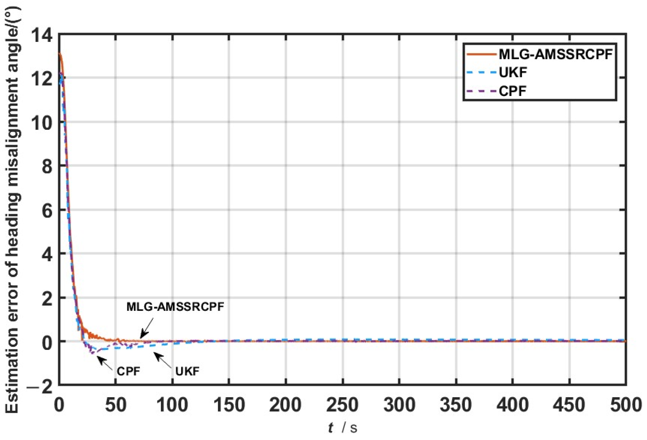
Since the roll and pitch misalignment angles are small, the filtering algorithm will converge quickly. Therefore, only the simulation results of the heading misalignment angle are presented below.

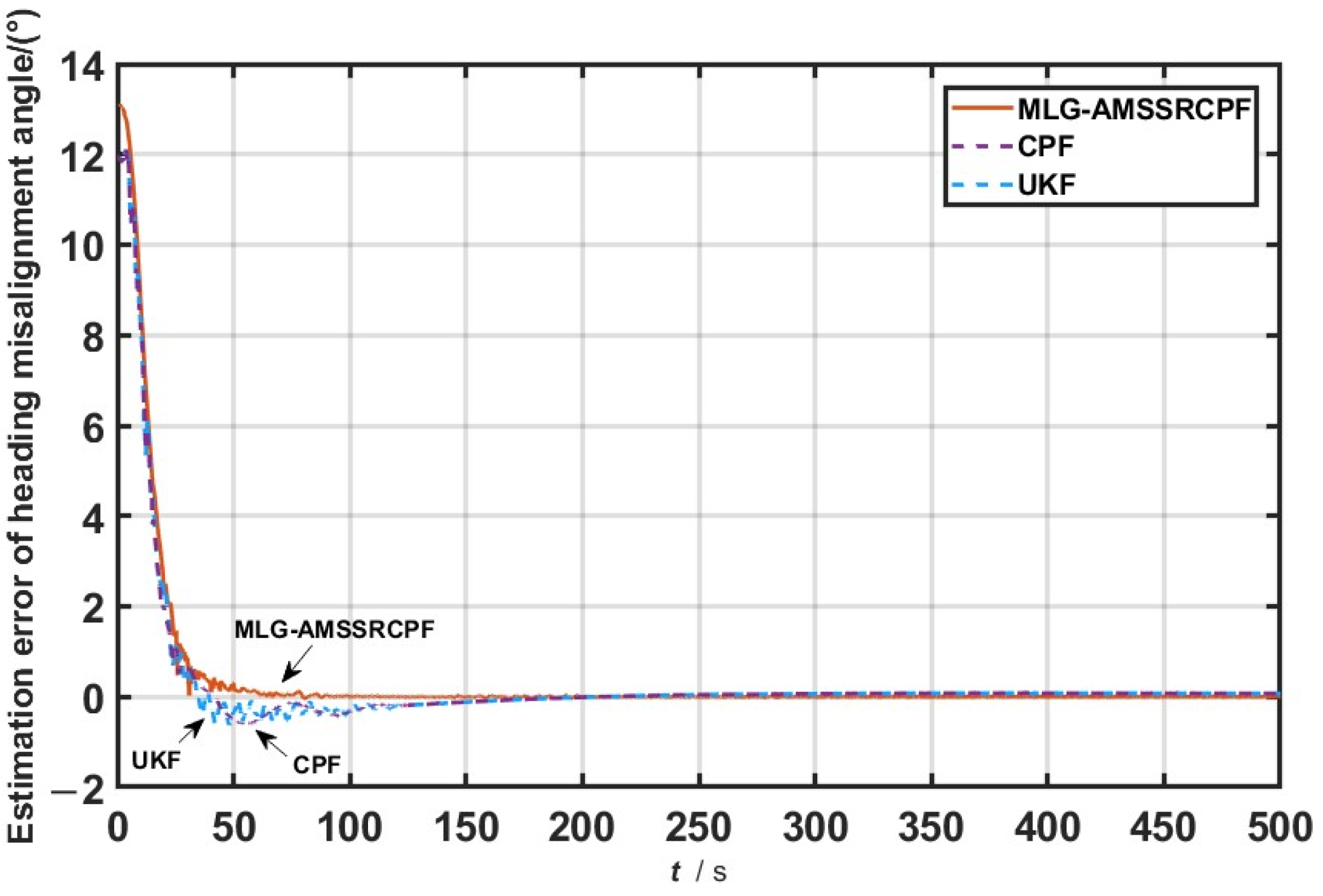
The filtering results for these three scenarios are shown in Figure 4, Figure 5 and Figure 6.

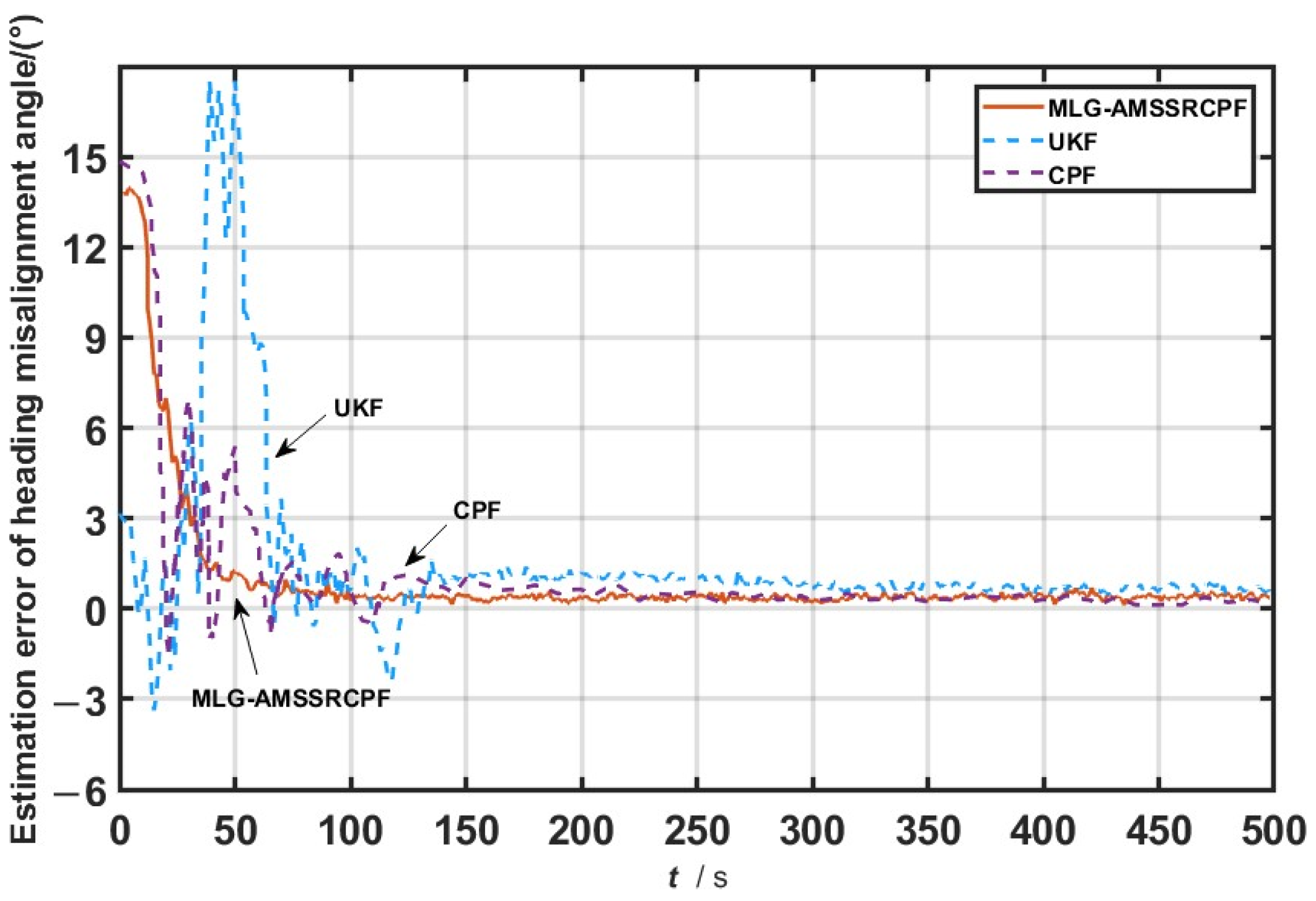
As shown in Figure 4, when the system model operates under normal conditions without any anomalies, the filtering performances of the CPF, UKF, and MLG-AMSSRCPF algorithms are highly similar. This is primarily due to the inherent randomness in the particle generation process, which introduces only minor deviations in the filtering results. In Figure 5, where gross errors are present in the measurement data, the CPF and UKF algorithms exhibit noticeable fluctuations during the initial filtering phase. In contrast, the MLG-AMSSRCPF algorithm demonstrates significantly more stable performance, with minimal occurrences of abrupt “spikes”. This indicates that the proposed algorithm possesses a strong ability to mitigate the impact of measurement outliers, and thereby maintains the stability and reliability of the filtering process. Figure 6 shows that, when the system noise statistics are inaccurate, the MLG-AMSSRCPF algorithm still maintains a high level of estimation accuracy for the heading misalignment angle. In comparison, both the CPF and UKF algorithms fail to overcome the limitations caused by incorrect noise modeling, resulting in larger estimation errors and slower convergence rates. The estimation accuracies for all three simulation scenarios are summarized in

Table 2. Estimation accuracy of CPF, UKF, and MLG-AMSSRCPF algorithms.

Simulation Scheme	Misalignment Angle Error	UKF Estimation Error	CPF Estimation Error	MLG-AMSSRCPF Estimation Error	UKF Alignment Time	CPF Alignment Time	MLG-AMSSRCPF Alignment Time
scheme one	heading	4.96′	4.82′	4.39′	115 s	81 s	65 s
scheme two	heading	15.86′	9.58′	6.58′	142 s	138 s	82 s
scheme three	heading	12.75′	8.72′	5.25′	162 s	160 s	88 s

Note: Misalignment angle error is expressed in arcminutes (′), and alignment time is expressed in seconds (s).

.

From Table 2, it can be seen that the MLG-AMSSRCPF algorithm effectively mitigates the impacts of gross measurement errors and system noise uncertainty, thereby exhibiting an improved estimation accuracy.

As shown in Table 2, the MLG-AMSSRCPF algorithm consistently outperforms both the CPF and UKF algorithms in terms of its estimation accuracy across all three simulation scenarios. In particular, under Scenario 2 and Scenario 3, the MLG-AMSSRCPF algorithm demonstrates significantly stronger suppression capabilities than the CPF algorithm when dealing with measurement outliers and inaccurate system noise statistics. Specifically, in Scenario 1, the heading error of the MLG-AMSSRCPF algorithm is reduced by 8.91% compared to that of CPF. In Scenario 2, the reduction reaches 31.29%, and in Scenario 3, it further improves to 39.79%. In addition, when compared with the UKF algorithm, the MLG-AMSSRCPF algorithm also exhibits enhanced robustness and adaptability in all three scenarios. The heading error is reduced by 11.49% in Scenario 1, 58.52% in Scenario 2, and 58.82% in Scenario 3. These results clearly demonstrate the robustness and adaptability of the MLG-AMSSRCPF algorithm in complex dynamic environments, highlighting its strong potential for practical application in high-precision state estimation tasks.

7. Experimental Validation

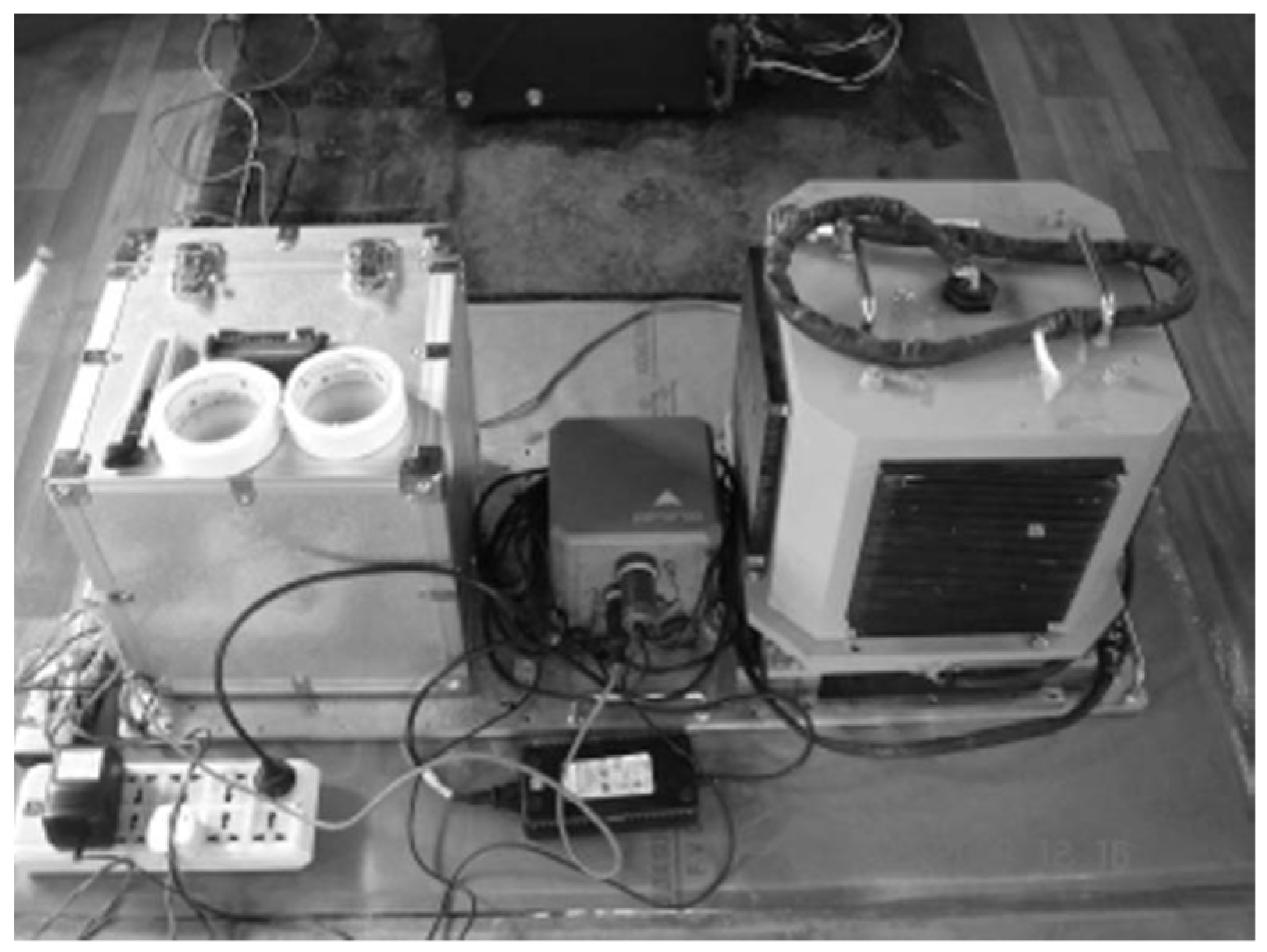
To further verify the practical feasibility of the proposed MLG-AMSSRCPF algorithm for the initial alignment of underwater vehicles on a marine dynamic platform, a comparative experiment was conducted using real-world measurement data obtained from a sea trial. The traditional CPF and UKF algorithms, along with the proposed MLG-AMSSRCPF algorithm, were applied for comparative analysis. The installation layout of the experimental equipment is illustrated in Figure 7. As shown, the ballast box is positioned on the left, the Doppler velocity log (DVL) is mounted in the center, and the fiber optic gyroscope is located on the right.

The performance specifications of the fiber optic gyroscope (FOG) are as follows: dynamic range of $\pm 100^{°}/s$; zero bias stability ≤ 0.005°/h; random walk ≤ 0.001°/h; calibration factor ≤ 5 ppm. The performance specifications of the accelerometer are as follows: dynamic range of ±4 g; zero bias stability ≤ 1 × 10⁻⁵ g. The performance specifications of the DVL are as follows: measurement accuracy of 0.01 m/s, measurement range of 0–10 m/s, measurement frequency of 2 Hz, and system error of ±0.02 m/s. The offshore motion-base alignment test was conducted in Qingdao, China, at a latitude of 35.98° N and longitude of 120.20° E. A total of 10 motion-base alignment trials were completed in a free navigation state. Offline semi-physical simulations were performed on the raw data collected during the trials. Since the alignment time was short, it was assumed that the gyro error consisted of constant drift and white noise, while the accelerometer error was modeled as a zero-bias with white noise. Out of the 10 trials, 8 trials showed that the MLG-AMSSRCPF algorithm outperformed the CPF and UKF algorithms, while the alignment results in the remaining 2 trials were similar. 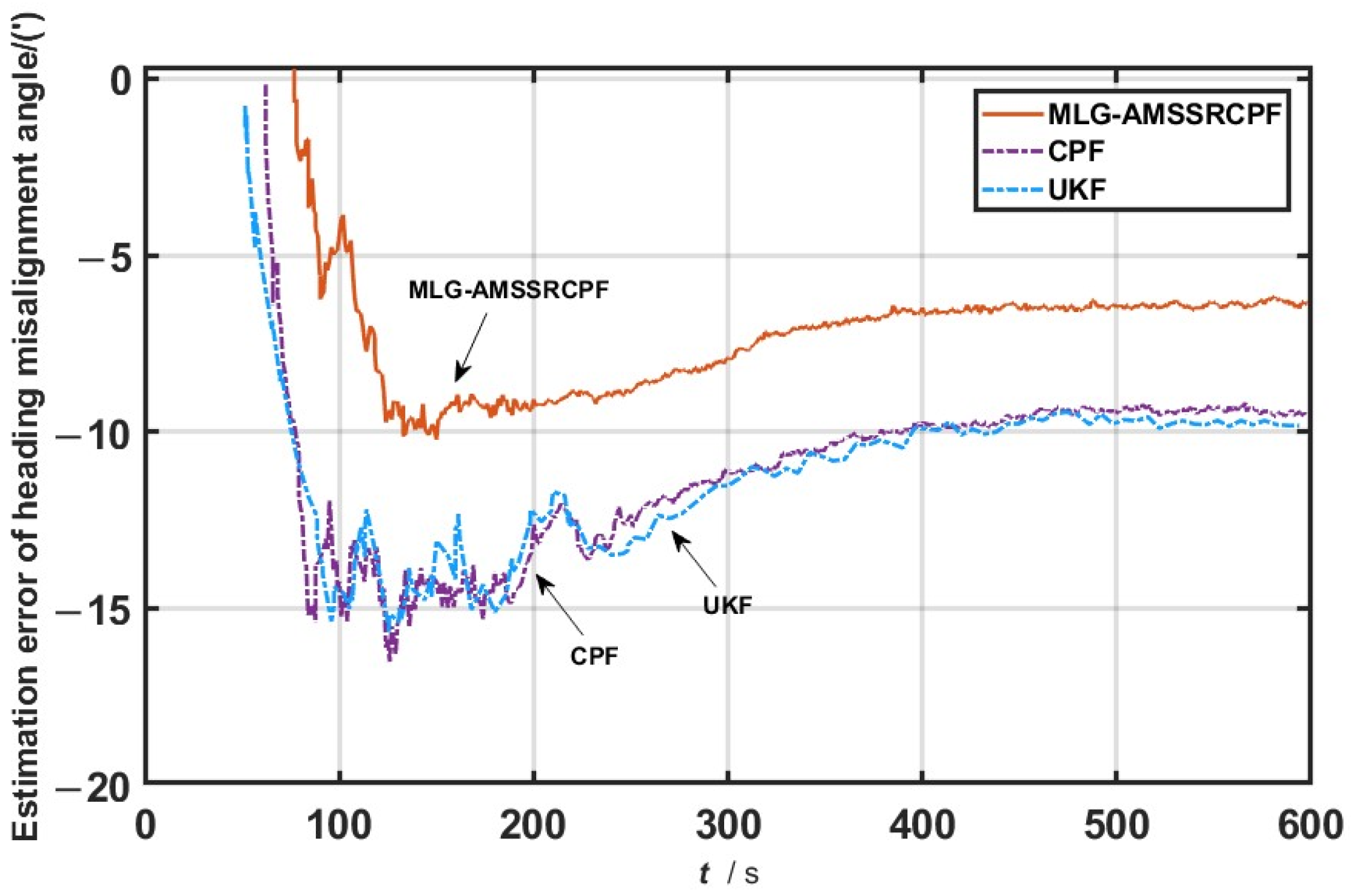Figure 8 displays the heading misalignment angle estimation error curve from one of the 10 trials, and the average estimation errors of both algorithms are shown in

Table 3. The alignment results based on UKF, CPF, and MLG-AMSSRCPF algorithms.

Filtering Method	Estimation Error of Heading Misalignment Angle/(′)	Alignment Time/(s)
UKF	9.96′	472 s
CPF	9.52′	465 s
MLG-AMSSRCPF	6.78′	320 s

.

In this experiment, the Doppler Velocity Log (DVL) exhibited brief velocity spikes, resulting in outliers within the measurement data. Additionally, due to sea-state disturbances, the gyroscope bias showed slight fluctuations during the alignment process, indicating non-ideal characteristics in the system noise statistics. These phenomena were observed across multiple trials, confirming the presence of real measurement outliers and noise uncertainty under the experimental conditions.

From the motion-base alignment test results presented in Figure 8 and Table 3, it is evident that the proposed MLG-AMSSRCPF algorithm achieves significantly higher alignment accuracy than the traditional CPF and UKF algorithms. According to the data in Table 3, in one of the sea trials, the average estimation error of the heading misalignment angle using MLG-AMSSRCPF was 6.78′, representing a 28.8% reduction compared to the 9.52′ obtained with the CPF algorithm. Furthermore, compared to the UKF algorithm, which exhibited an average error of 9.96′, the MLG-AMSSRCPF algorithm achieved an improvement of approximately 31.9%. This notable enhancement in alignment performance is primarily attributed to the algorithm’s robust capability to manage anomalous measurement data and inaccuracies in the statistical properties of system noise during the motion-base alignment process.

During the motion-base alignment process, measurement data may be disturbed by external factors, leading to gross errors in the resulting observations, while uncertainties in system noise characteristics may introduce additional errors. The traditional CPF and UKF algorithms are quite sensitive to these issues, which results in decreased estimation accuracy and stability. In contrast, the MLG-AMSSRCPF algorithm effectively mitigates the impact of measurement outliers and achieves an enhanced adaptability to variations in system noise through the introduction of a matrix Lie group-based error optimization mechanism, mixed-order sampling, adaptive noise covariance adjustment, and self-adjusting particle count and weight strategies. These features enable the algorithm to provide higher alignment accuracy and faster convergence in complex dynamic marine environments, fully demonstrating its robustness and superior performance in practical applications.

8. Conclusions

This paper addresses the nonlinear filtering challenges associated with the initial alignment of underwater vehicles’ motion bases under large heading misalignment conditions. We propose a matrix Lie group-based adaptive mixed-order spherical simplex-radial volume sampling particle filter (MLG-AMSSRCPF). By combining the exponential and logarithmic mappings of the matrix Lie group SO(3), the algorithm enables the accurate transformation of attitude errors between manifold space and Euclidean space, thereby avoiding the complexity of computing the Jacobian matrix for rotational motion and significantly reducing model linearization errors. The introduction of the MSSR volume sampling rule enhances the algorithm’s precision compared to the CKF, while significantly reducing its computational complexity compared to the HCKF. This method not only improves the accuracy of state mean and covariance propagation but also optimizes the algorithm’s computational efficiency. Furthermore, the dynamic particle count adjustment strategy, combined with the multi-dimensional Huber loss function, effectively suppresses the impacts of outliers and further enhances the robustness and computational efficiency of the filter.

In simulation experiments, the MLG-AMSSRCPF algorithm demonstrates outstanding estimation accuracy and convergence performance under various typical operating conditions, such as normal measurements, gross measurement errors, and sudden changes in system noise. Compared with the traditional CPF and UKF algorithms, the MLG-AMSSRCPF algorithm achieves an improvement of approximately 9–62% in its heading misalignment angle estimation accuracy, showing especially higher adaptability and anti-jamming capabilities in complex noise environments. These simulation results validate the effectiveness and superiority of the proposed algorithm in addressing complex nonlinear scenarios.

Verification based on real-world offshore motion-base alignment experiments further demonstrates the practical applicability and engineering potential of the proposed MLG-AMSSRCPF algorithm. Across 10 experimental trials, the MLG-AMSSRCPF algorithm consistently outperformed the traditional CPF and UKF algorithms in most cases. It effectively mitigated the effects of gross measurement errors and uncertainties in system noise statistics, while significantly enhancing the accuracy and robustness of motion-base initial alignment. In the sea trials, the heading misalignment angle estimation error of the MLG-AMSSRCPF algorithm was reduced by 28.8% compared to that of the CPF algorithm, and by 31.9% compared to that of the UKF algorithm, further validating its strong adaptability to complex and dynamic environments. The proposed algorithm provides a novel and effective solution for allowing the high-precision navigation of underwater vehicles operating in challenging conditions, and holds significant value for real-world engineering applications. Future research can further explore the extension of this algorithm to scenarios involving multi-sensor fusion, high-dynamic nonlinear systems, and real-time computation, to meet the growing demands of next-generation precision navigation systems and to promote the continued advancement of nonlinear filtering techniques.

References

1. Zhu, S.J. Technique review of alignment for inertial navigation systems with moving base. Control Technol. Tactical Missile 2004, 4, 46–49. [Google Scholar]
2. Yan, G.M.; Weng, J.; Bai, L. Initial in-movement alignment and position determination based on inertial reference frame. Syst. Eng. Electron. 2011, 33, 618–621. [Google Scholar]
3. Shen, S.Y.; Mulgaonkar, Y.; Kumar, V. Vision-based state estimation and trajectory control towards high-speed flight with a quadrotor. In Proceedings of the Robotics: Science and Systems (RSS), Berlin, Germany, 24–28 June 2013; pp. 1157–1165. [Google Scholar]
4. Kelly, J.; Sukhatme, G.S. Visual-inertial sensor fusion: Localization, mapping, and sensor-to-sensor self-calibration. Int. J. Robot. Res. 2011, 30, 56–79. [Google Scholar] [CrossRef]
5. Engel, J.; Schöps, T.; Cremers, D. Large-scale direct SLAM with stereo cameras. In Proceedings of the Intelligent Robots and Systems (IROS), Hamburg, Germany, 28 September–3 October 2015; pp. 1935–1942. [Google Scholar]
6. Grewal, M.S.; Weill, L.R.; Andrews, A.P. Global positioning systems, inertial navigation, and integration. Wiley Interdiscip. Rev. Comput. Stat. 2007, 3, 383–384. [Google Scholar] [CrossRef]
7. Marins, J.L.; Yun, X.; Bachmann, E.R.; McGhee, R.B.; Zyda, M.J. An extended Kalman filter for quaternion-based orientation estimation using MARG sensors. In Proceedings of the Intelligent Robots and Systems, Maui, HI, USA, 29 October–3 November 2001; pp. 2003–2011. [Google Scholar]
8. Wang, D.L.; Zhang, H.Y. Nonlinear filtering algorithm for INS initial alignment. J. Chin. Inert. Technol. 1999, 7, 17–21. [Google Scholar]
9. Gu, D.Q.; Qin, Y.Y. Unscented Kalman filter for in-motion alignment of shipborne SINS. Syst. Eng. Electron. 2006, 28, 1218–1220. [Google Scholar]
10. Arasaratnam, L.; Haykin, S. Cubature Kalman Filters. In Proceedings of the Transactions on Automatic Control, Istanbul, Turkey, 30 May–1 June 2009; pp. 1254–1269. [Google Scholar] [CrossRef]
11. Doucet, A.; Godsill, S.; Andrieu, C. On sequential Monte Carlo sampling methods for Bayesian filtering. Stat. Comput. 2000, 10, 197–208. [Google Scholar] [CrossRef]
12. Cheng, C.; Ansari, R. Kernel particle filter for visual tracking. IEEE Signal Process. Lett. 2005, 12, 242–245. [Google Scholar] [CrossRef]
13. Gordon, N.J. A hybrid bootstrap filter for target tracking in clutter. IEEE Trans. Aerosp. Electron. Syst. 1997, 33, 353–358. [Google Scholar] [CrossRef]
14. Ning, X.; Huang, P. Adaptive points range square-root cubature Kalman filter for Mars approach navigation. In Proceedings of the 33rd Chinese Control Conference, 28–30 July 2014; pp. 903–908. [Google Scholar]
15. Liu, F.; Li, X.; Zhang, Y. Cubature particle filter optimized by adaptive MSSRCKF for SINS/GNSS navigation. IEEE Trans. Aerosp. Electron. Syst. 2023, 59, 210–223. [Google Scholar]
16. Cheng, X.H.; Li, B.L.; Wang, Y. SINS Initial Alignment on Moving Bases Based on Particle Filter. J. Chin. Inert. Technol. 2009, 17, 267–271. [Google Scholar]
17. Chui, M. Research on Initial Alignment Method for Large Azimuth Misalignment Angle Based on CQKF. Master’s Thesis, Harbin Engineering University, Harbin, China, 2015. [Google Scholar]
18. Sun, F.; Tang, L. Initial Alignment of Large Azimuth Misalignment Angle in SINS Based on CKF. Chin. J. Sci. Instrum. 2012, 33, 327–333. [Google Scholar]
19. Yan, D.; Yu, W.; Song, Y.; Wu, C.; Song, Y. A new method for visual inertial odometry based on matrix Lie group representation and cubature Kalman filter. Control Decis. 2020, 35, 1823–1832. [Google Scholar]
20. Yang, Y.; Gao, W. An Optimal Adaptive Kalman Filter. J. Geod. 2006, 80, 177–183. [Google Scholar] [CrossRef]
21. Yang, Y.; Gao, W. Comparison of Two Fading Filters and Adaptively Robust Filter. Geo-Spat. Inf. Sci. 2007, 10, 200–203. [Google Scholar] [CrossRef]
22. Liao, T.; Jing, Z.; Li, M.; Pan, H. An adaptive visual/inertial integrated navigation algorithm based on Lie groups. Inf. Control 2020, 49, 585–590, 597. [Google Scholar] [CrossRef]
23. Condurache, D.; Șfartz, E. Exact Closed-Form Solutions of the Motion in Non-Inertial Reference Frames, Using the Properties of Lie Groups SO3 and SE3. Symmetry 2021, 13, 1963. [Google Scholar] [CrossRef]
24. Takayama, Y.; Urakubo, T.; Tamaki, H. Adaptive selection of process noise covariance in Kalman filter using measurement matrix. IEEE Trans. Control Syst. Technol. 2023, 31, 2451–2462. [Google Scholar]
25. Hu, Y.; Peng, A.; Tang, B.; Xu, H. Adaptive cubature Kalman filter for inertial/geomagnetic integrated navigation system based on long short-term memory network. Sensors 2021, 14, 5905. [Google Scholar]
26. Shen, W.; Liu, J. Design of robust cubature fission particle filter algorithm in multi-source cooperative navigation. Sci. Rep. 2022, 12, 4210. [Google Scholar]
27. Jia, H.; Wang, L. A robust particle filtering algorithm with adaptive particle number for nonlinear systems. J. Guid. Control Dyn. 2021, 44, 314–326. [Google Scholar] [CrossRef]
28. Liu, F.; Zheng, X. Efficient particle filter design for GPS/SINS integrated navigation systems with improved resampling. IEEE Trans. Aerosp. Electron. Syst. 2022, 58, 174–188. [Google Scholar]
29. Yang, X.; Wu, T. Adaptive filter design using Mahalanobis distance for robust estimation in GNSS/INS integration. Sensors 2020, 20, 2434. [Google Scholar]
30. Zhao, Y.; Cheng, D. Study of robust filtering methods in complex navigation environments with gross errors. Measurement 2019, 140, 123–132. [Google Scholar] [CrossRef]
31. Wang, Z.; Li, J. Application of adaptive filtering in high-dimensional sensor fusion systems. IEEE Sens. J. 2023, 23, 3524–3534. [Google Scholar]
32. Smith, J.; Brown, C. Huber loss in high-dimensional filtering for nonlinear systems. J. Signal Process. Syst. 2020, 92, 78–89. [Google Scholar]
33. Chen, K.; Zhang, Y. Robust particle filtering using adaptive Huber loss function for GNSS-based navigation systems. IEEE Access 2021, 9, 65432–65441. [Google Scholar]
34. Wang, S.; Feng, Y.; Duan, S.; Wang, L. Mixed-Degree Spherical Simplex-Radial Cubature Kalman Filter. Math. Probl. Eng. 2017, 2017, 6969453. [Google Scholar] [CrossRef]
35. Xu, X.; Tian, Z.; Liu, Y.; Zou, H. SINS Initial Alignment Method Based on an Improved CKF. J. Huazhong Univ. Sci. Technol. 2016, 44, 81–86. [Google Scholar] [CrossRef]
36. Cui, B.; Wei, X.; Chen, X.; Wang, A. Improved high-degree cubature Kalman filter based on resampling-free sigma-point update framework and its application for inertial navigation system-based integrated navigation. Aerosp. Sci. Technol. 2021, 117, 106905. [Google Scholar] [CrossRef]
37. Hao, S.; Lu, H.; Wei, X.; Xu, M. Simplified High-Order Strong Tracking Cubature Kalman Filter and Its Application in Integrated Navigation. Control Decis. 2019, 34, 2105–2114. [Google Scholar] [CrossRef]
38. Wang, N.; Liu, F. Application of constrained optimization-based adaptive fading memory MSSRCPF filtering in SINS/GNSS integrated navigation. Meas. Control 2024, 54, 3660–3672. [Google Scholar] [CrossRef]
39. Zhang, Y.; Xin, M.; Fang, H. Filtering Structures for α-Stable Systems. IEEE Control Syst. Lett. 2023, 7, 292–297. [Google Scholar] [CrossRef]
Figure 1. The schematic of moving base initial alignment.
Information 16 00416 g001
Figure 2. MLG-AMSSRCKF filtering algorithm flowchart.
Information 16 00416 g002
Figure 3. MLG-AMSSRCPF algorithm flowchart.
Information 16 00416 g003
Figure 4. Estimation error of heading misalignment angle (scheme one).
Information 16 00416 g004
Figure 5. Estimation error of heading misalignment angle (scheme two).
Information 16 00416 g005
Figure 6. Estimation error of heading misalignment angle (scheme three).
Information 16 00416 g006
Figure 7. The moving based alignment test system.
Information 16 00416 g007
Figure 8. Estimation error curve of heading misalignment angle.
Information 16 00416 g008