Generating Human-Interpretable Rules from Convolutional Neural Networks

Abstract

Advancements in the field of artificial intelligence have been rapid in recent years and have revolutionized various industries. Various deep neural network architectures capable of handling both text and images, covering code generation from natural language as well as producing machine translation and text summaries, have been proposed. For example, convolutional neural networks or CNNs perform image classification at a level equivalent to that of humans on many image datasets. These state-of-the-art networks have reached unprecedented levels of success by using complex architectures with billions of parameters, numerous kernel configurations, weight initialization, and regularization methods. Unfortunately to reach this level of success, the models that CNNs use are essentially black box in nature, with little or no human-interpretable information on the decision-making process. This lack of transparency in decision making gave rise to concerns amongst some sectors of the user community such as healthcare, finance, justice, and defense, among others. This challenge motivated our research, where we successfully produced human-interpretable influential features from CNNs for image classification and captured the interactions between these features by producing a concise decision tree making that makes classification decisions. The proposed methodology makes use of a pretrained VGG-16 with fine-tuning to extract feature maps produced by learnt filters. On the CelebA image benchmark dataset, we successfully produced human-interpretable rules that captured the main facial landmarks responsible for segmenting men from women with 89.6% accuracy, while on the more challenging Cats vs. Dogs dataset, the decision tree achieved 87.6% accuracy.

1. Introduction

Artificial intelligence has made significant progress, especially in recent years, where it has undergone unprecedented development and revolutionized various fields and industries by improving productivity in virtually every sector of Industry. Transitioning from a theoretical concept in the early 1950s [1], it has become a mainstream technology reaching a broader audience, through different applications used on a day-to-day basis. For instance, the recent surge in the usage of large language models capable of generating code from natural language, producing machine translations, and performing text summarizations exemplifies the advancements in this field, benefiting not only professionals but the general public as well.

In the last decade, a plethora of deep neural network architectures have been proposed, with increasing complexities and greater depth in terms of layers. In addition, different kernel configurations, utilizing several different weight initialization and regularization methods, enabled the use of deep learning with depths reaching thousands of layers with billions of learned parameters. These sophisticated architectures and techniques helped to reach unprecedented success on different benchmark tasks like ILSVRC [2] or CIFAR [3]. However, this race towards perfection with highly complex architectures [4,5,6,7,8] also transitioned the models into black-box entities, which provided little or no information on the decision-making process employed by these models. These models, although performing very well in terms of accuracy, were opaque, and the challenges with interpretation or explainability started raising concerns [9,10,11,12].

For some industries, such as healthcare, security, finance, and justice, transparency in decision making is equally important to, if not more so than, accuracy. For instance, in healthcare, a deep learning model’s diagnosis with high accuracy provides an insight; however, explaining the decision-making process or the logic behind that conclusion is equally important to understand to be acceptable and trustworthy to end users. Introducing interpretability in complex models addresses transparency needs and bridges the gap between high performance and the explainability of the decision-making process. Explorations and improvements have given rise to a vigorous, yet nascent, field of research known as explainable artificial intelligence (XAI) which seeks to enhance transparency, accountability and trust in AI systems [13,14].

The research on XAI [15,16,17,18,19] has achieved partial success in explaining the decisions made by CNNs in the application domain area of image classification. The focus has been on using feature maps to explain the decisions made by the classifier at the output layer. Some examples include local explainable AI (XAI) methods such as layer-wise relevance propagation (LRP) [17], global XAI techniques providing insights through visual explanations (heatmaps) and model inspection, and an even more recent work, concept relevance propagation (CRP) [18], which extends LRP to provide feature maps with richer content, which in turn provides for more accurate explanations of the classification decisions made.

Despite the surge of interest in XAI, there has been no attempt so far at capturing the interactions between different features (in the form of feature maps). Local models focusing on individual features and recording their contribution in classifying images are useful in their own right but do not provide a comprehensive explanation of why one image is classified, for example, as a cat whereas another is categorized as a dog. What differentiates one type of image from another is a set of features, along with the interactions between them. The objective of this research is to propose and validate a methodology that produces a transparent model that explains how classification decisions are made based on the set of features used and the interactions between them. The proposed methodology automatically extracts features from images and then constructs a decision tree based on this features that traces how classification decisions are made by following a decision path from the root of the tree down to the leaf node that identifies the class of the image.

2. Materials and Methods

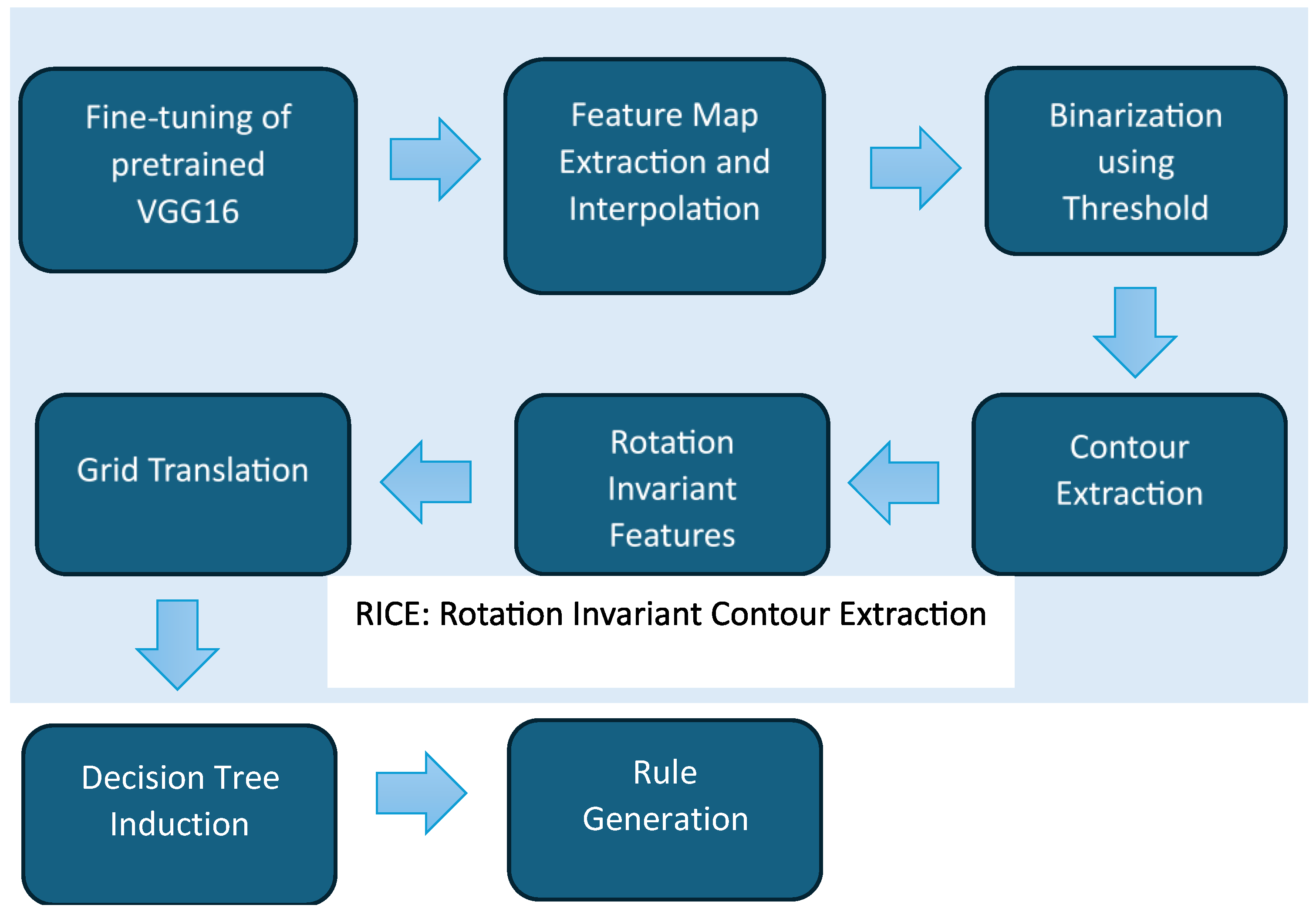
2.1. Overview of Methodology

Our methodology uses a 2-phase process shown in Figure 1. In phase 1, features are extracted from a CNN classification model. We describe our feature extraction method with reference to the VGG-16 [19] architecture, although our feature extraction method is generic and can be used with any CNN architecture.

We used the weights obtained by training a VGG-16 model on the benchmark Imagenet dataset [2]. VGG-16 is a 16-layer CNN that has been extensively used in prior deep neural network research on image classification. VGG-16’s architecture is hierarchical in nature in the sense that it progressively generates more feature maps with increasing depth of the layers, as Figure 2 illustrates. This enables it to capture more fine-grained image features, which are then fed into the 3 dense layers for classification at the end of the last convolutional block of layers.

One of the critical decisions that need to be made in using any pretrained model is to determine the cutoff point at which the set of weights obtained from Imagenet training is frozen. One extreme is retraining from layer 1 onwards, which effectively means that the entire set of weights and feature maps are learnt from layer 1 onwards. At the other extreme is setting the cutoff at layer 16, which means that the weights from the VGG-16 model learned from Imagenet are deployed with no modification. The other extreme is to learn weights from layer 1 itself, which means that the entire CNN is retrained with the custom dataset that is to be targeted for classification. Determining the ideal cutoff point directly affects the number of feature maps that discriminate between the classes. Too high a cutoff point yields a larger number of feature maps with non-zero values, potentially increasing the risk of overfitting. On the other hand, too low a cutoff point has the opposite effect of producing too few feature maps that actually contribute to the classification process.

As our explanatory model is based on a decision tree classifier, it is of critical importance to limit the number of features fed into the decision tree classifier in order to produce a human-interpretable model. Thus, fine-tuning provides opportunities not just for improving interpretability for the decision tree model produced downstream but also for potentially reducing the risk of model overfitting. Fine-tuning was implemented varying the cutoff point until the classification accuracy on the validation set was maximized. This yielded a value of 13 for both of the datasets used in this study. We elaborate on this process in the detailed discussion that follows in Section Feature Extraction from Feature Maps. More details on the methodology, including the fine-tuning process, is provided in [20].

In the next step, the feature maps identified through fine-tuning were processed to extract features. Feature maps were represented by 2-dimensional arrays, and these arrays had to be further processed to obtain scalar valued features that could be fed into a decision tree model. The details of the transformation from 2D arrays to scalar form are presented in Section Feature Extraction from Feature Maps.

In phase 2, the scalar features extracted were used to induce a decision tree model, which was followed by encoding the decisions made at the leaf nodes of the tree with symbolic rules that were human-interpretable.

2.2. Feature Extraction and Rule Generation

We describe the details of feature selection in Section Feature Extraction from Feature Maps and then describe the rule generation processes in Section 3.3.

Feature Extraction from Feature Maps

As described above, the strategy used in feature extraction involved obtaining a small number of feature maps by tuning the number of layers (k) that were retrained using the target custom dataset. This resulted in reducing the number of feature maps responsible for classification from 512 to 3 for the Celeba dataset and to 2 for the Cats vs. Dogs dataset. The value of k ranged between 1 (the layer closest to the first dense classification layer) to 3 (the layer furthest away from the dense layers) in block 5 of the VGG-16 architecture. The k value that yielded the highest accuracy on the validation dataset was used to identify the feature maps that were ultimately used in the feature extraction process. We observed in our experimentation that the optimal value of k produced a certain number of feature maps that consisted entirely of zero values. These feature maps were filtered out, and the remaining maps were selected for feature extraction, as outlined in Figure 1 and further described in Section 3.3.1. We also validated the subset of feature maps that were selected against the set of feature maps F produced by VGG-16 without tuning, i.e., the original features maps at the last convolutional layer. With n as the number of feature maps produced by fine-tuning, we randomly selected 2n, 3n, 4n, …, mn feature maps from F, and then, for each subset selected we again evaluated the accuracy across the validation set. The integer m is given by m = floor(128/n) from set F, where floor returns the smallest multiple of n that is smaller than 128.ationale here was to demonstrate that the features returned from fine-tuning were far superior to randomly selecting up to a large fraction (25%) of the features from the original VGG-16 model without fine-tuning. In both datasets that we experimented with, we found that the feature maps returned from feature selection were far superior to those of random selection from the original set F. In Section 3, we present the detailed results of this experiment.

The next step of the methodology was applying bilinear interpolation [21] to scale each feature map (which was sized 7 by 7 for VGG-16) to the size of the original images (which were sized 128 by 128) for both of the datasets that we used. Interpolation is the process of fitting a linear model to a set of data points in space and then inferring the numerical value of the points not covered by the samples provided in the training data. Bilinear interpolation is a variant of linear interpolation that is applied to 2-dimensional space and is thus appropriate for image processing.

The intention here was to superimpose selected feature maps on the source images. Such superposition enabled us to identify which regions from the source images were responsible for classification by the CNN model. Having performed the superposition, we next performed a binarization operation to isolate significant regions from non-significant ones. To implement this, we used a threshold of 95% on the intensity of the pixels to binarize the image. That is, we selected 5% of the brightest pixels from the superposed image to identify the areas of each image that were critical for classification by the CNN, which we term the critical region.

The contours of the critical region were then extracted for each feature map that yielded irregular shapes that could not be easily represented by scalar features. To produce scalar features, we constructed the minimum bounding box that enclosed the critical region. The minimum bounding box was obtained by applying the convex hull algorithm that returned the minimum enclosing rectangle that spanned a given set of points in space. We used the OpenCVs implementation of the convex hull algorithm for this purpose.

With the minimum bounding box in place, we computed three scalar measures from it, namely, aspect ratio, perimeter, and area. These three measures taken together provided the rotation invariancy of the critical region as they captured the inherent geometry that was insensitive to the angular positioning of the critical region.

The final step in phase 1 was to provide locality information on critical regions relative to the dimensions of the original source image. To implement this, we divided the source image into a number of two-dimensional grids and then recorded the grid positions of each of the four vertices of the minimum bounding box. The motivation for this was to introduce interpretability into the features generated by providing spatial context that enables end users to understand the decision-making process. Thus, for example, on the CelebA dataset, a feature located in the central part of the face such as the cheek helped to distinguish between men and women. Introduction of spatial context in terms of easily identifiable face landmarks is a necessary and powerful method of introducing transparency into the decision-making process used by the CNN.

3. Results

We experimented with two different datasets, namely, the CelebA [22] and the Cats vs. Dogs [23] datasets.

3.1. System Configuration

All experiments were conducted in the Google Collab environment using a paid subscription plan granting access to premium Nvidia T4 GPUs without quota restrictions. Most of the experiments were executed using 15 GB of GPU memory and 12.7 GB of system memory in the Python 3 environment. In certain exceptional situations requiring high performance for testing purposes, 51 GB of RAM was utilized. However, having a high-memory system is not required, and a 15 GB GPU is sufficient to replicate the experiments (high memory was required for plotting the feature maps using matplotlib, and we could have used a 15 GB RAM configuration as well, albeit with a time penalty).

A MacBook Pro with Intel processor and 8 GB of RAM was used as a client machine to access Google Collab in Chrome and Safari browsers. A machine with at least 8 GB is recommended as the browser, as running Collab notebook uses up to 3 GB of memory in certain instances while plotting different feature maps.

3.2. Architecture Exploration

We present here the baseline CNN architecture that was used on both image datasets as a feature extractor. This baseline CNN used certain hyperparameters that were finalized after conducting numerous experiments. For example, the method used to reduce the number of features extracted in the last block of VGG-16 was training the last few convolutional layers with the custom dataset (CelebA [22] or Cats vs. Dogs [23]). However, the question of how many layers to train in order to generate the smallest number of meaningful feature maps to achieve accuracy well above that obtained through random selection was answered after multiple experimental runs covering multiple convolutional VGG-16 layers of the last 2 blocks.

Similarly, other important hyperparameters such as the number of dense layers; number of units in each dense layer; learning rate; requirement of the adaptive learning rate; number of epochs; early stopping, early stopping patience levels; optimizer; dimension of the input images; need for regularization covering L1, L2, and dropout; batch size; and train, test, and validation split were finalized after 100 s of experimental runs. Once these parameters were chosen from the experiments, the same values were used throughout all experiments for different datasets, unless otherwise mentioned specifically in the experiment subsection. These parameter values are given below in

Table 1. CNN architectural parameters used.

Parameter	Description and Value
VGG-16 trainable layers	Last 2 convolutional layers from Block 5
Number of dense layers used	2 dense layers, 1024 units in layer 1 and 512 in layer 2
Learning rate	0.0017
Epochs	50
Batch size	512
Early stopping	Yes, with patience value of 6
Optimizer	Adam
Input image shape	(128,128,3)
Train test validation split	For CelebA, there were 202,599 images in total, out of which 80% was used in training, 10% was used for validation, and 10% was used for testing. For the Cats vs. Dogs dataset, there were 25,000 images in total; the same ratios were used for training/validation/testing as for the CelebA dataset. Both datasets were balance with respect their classes.

for reference.

3.3. Experimental Study

For each dataset, we present the results of feature selection, image superposition, critical region extraction, feature generation, decision tree induction, and finally symbolic rule generation. Before we describe the experimentation in detail, we first present the system configuration we used to promote replicability.

We start with the experimentation on the CelebA dataset.

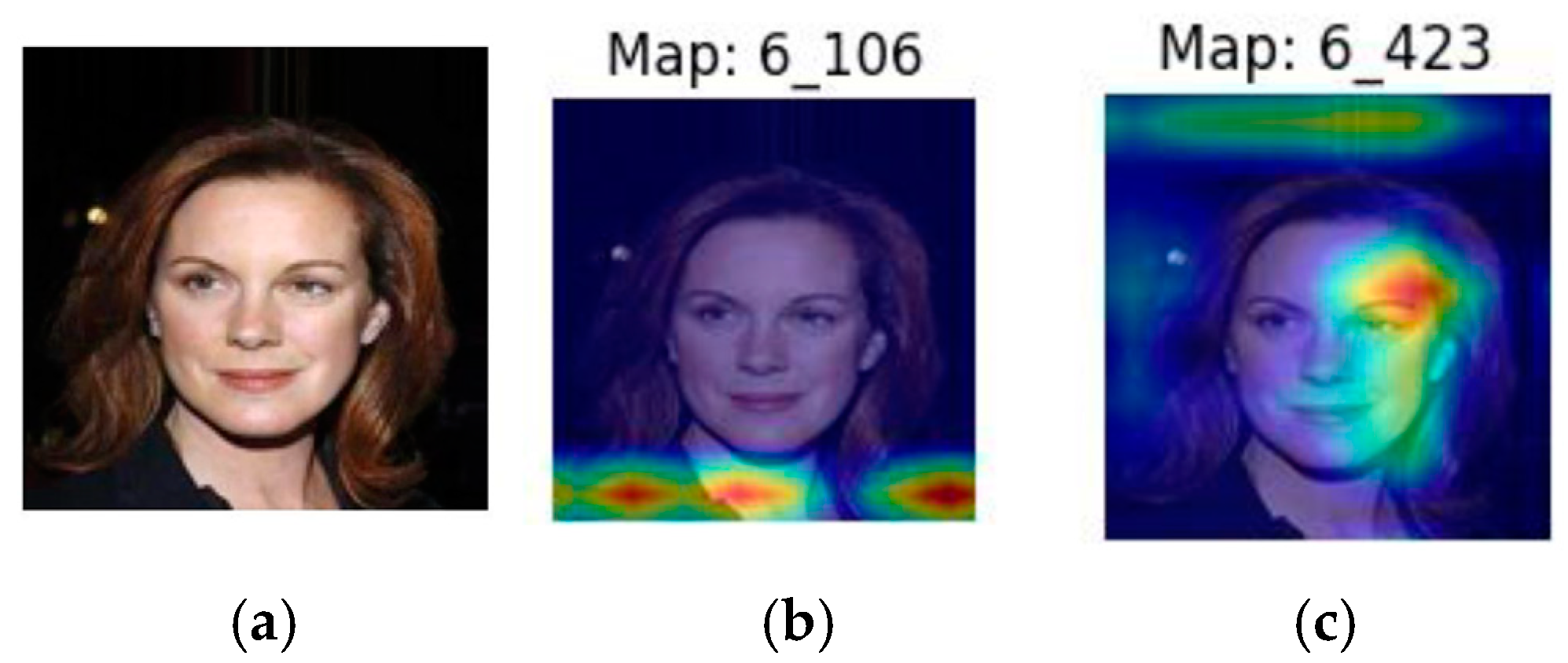
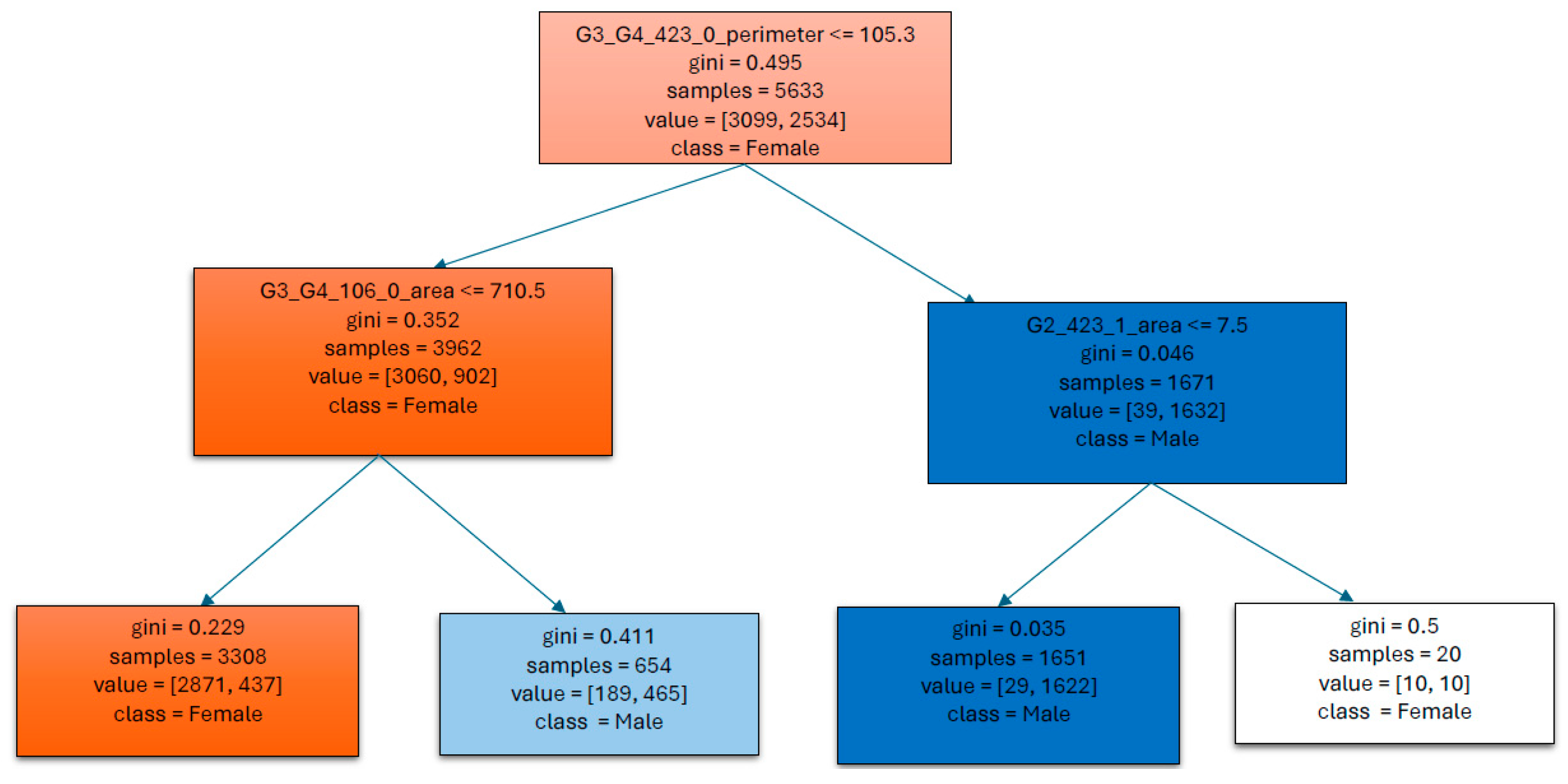
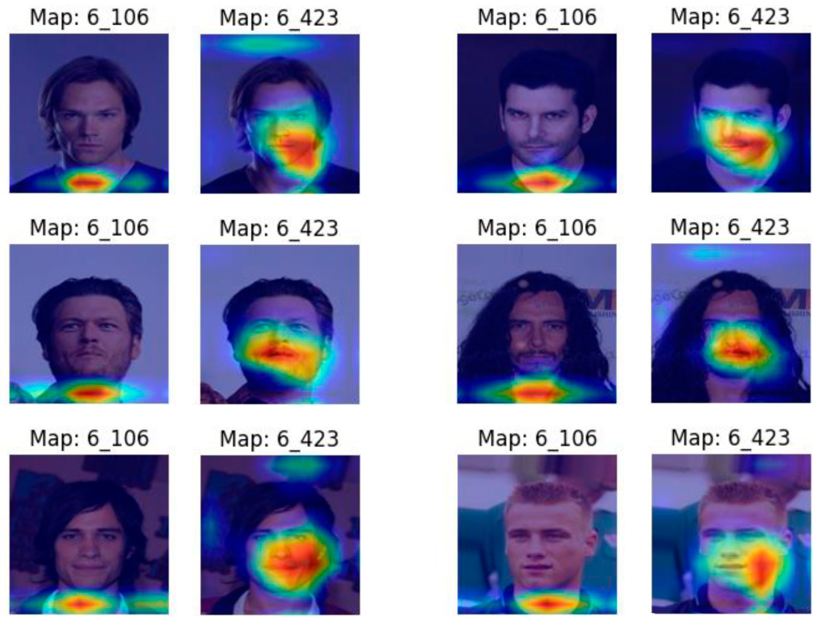
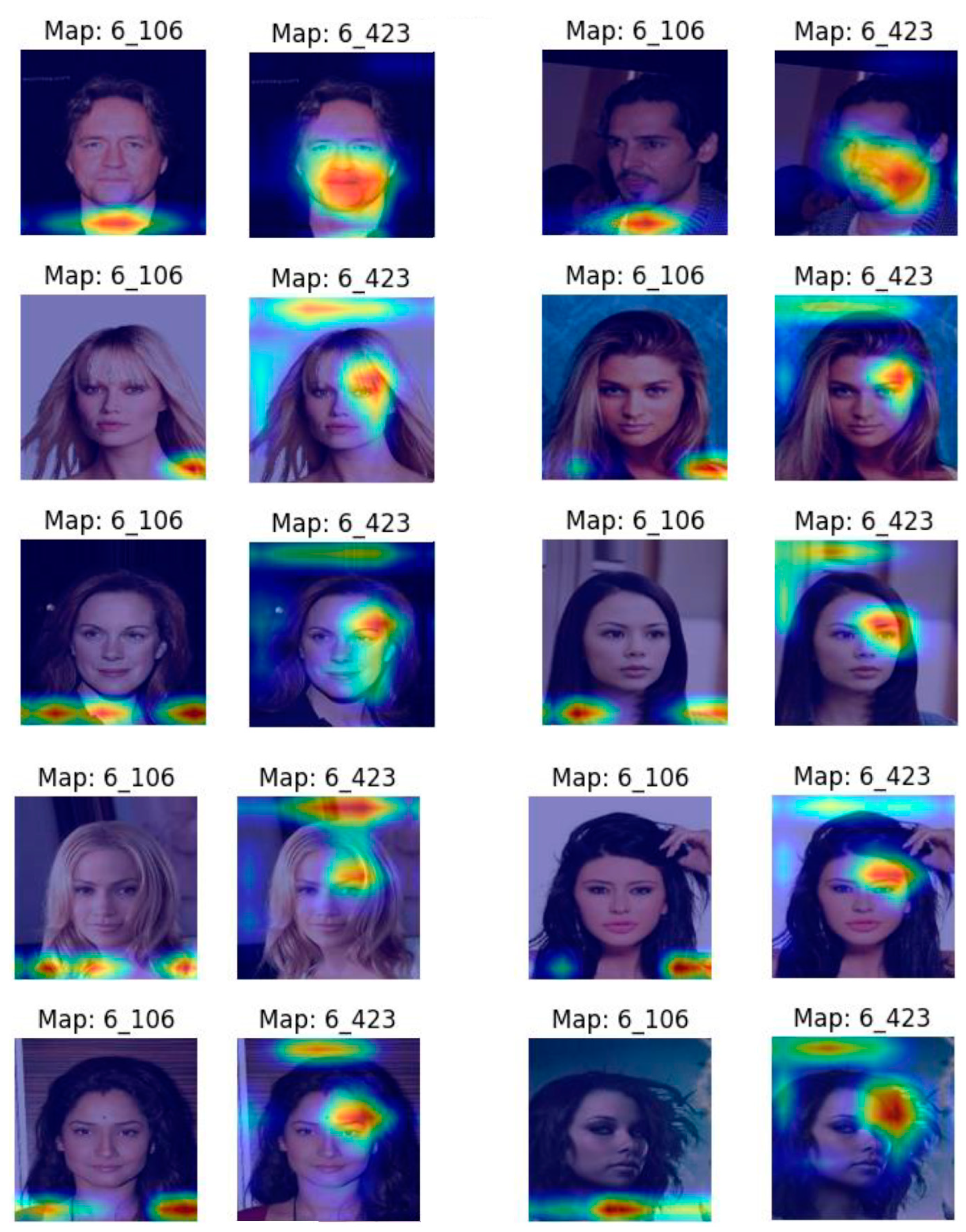
3.3.1. CelebA Case Study: Fine-Tuning, Feature Selection, and Image Superposition

As described in Section 2, fine-tuning was performed on the last two convolutional layers of the VGG-16 model, and the feature maps that had non-zero activation values were selected.

We now discuss in more detail the process of extracting features from the feature maps. Firstly, we created a new convolutional layer (layer 17) with 512 feature maps from the last dense layer (layer 16) of VGG-16. The fine-tuning resulted in layer 13 being identified as the best layer to learn weights from with the custom dataset. The fine-tuning process was highly effective as it resulted in just 2 of the 512 feature maps produced by layer 17 having non-zero activation values.

In the next step, bilinear interpolation, was applied on the feature maps to scale to the source image size to 128 by 128. Bilinear interpolation computes a new pixel value by taking a weighted average of the nearest 4 pixels surrounding the current pixel point to be interpolated. Other interpolation methods like bicubic or higher-order spline methods could also have been used for the rescaling operation. However, we chose bilinear interpolation as it was faster than other higher-order methods and thus efficiently met our requirement of identifying the pixels that contributed the most towards classification decisions by being the brightest (1 − t)% pixels from the source images, where t is a thresholding parameter. We refer to these regions as contours. In extracting contours from such regions, splitting was encountered in some cases, giving rise to two or more disjointed contours.

We experimented with different values of the thresholding parameter t in the range [80, 90, 95, 98] and finally chose 95 as it provided the best balance between validation accuracy and the number of contours generated. We factored in the number of contours as fewer contours leads to fewer features, which in turn enhances interpretability. Lower thresholds produced a smaller number of disjointed contours but reduced the accuracy whereas higher thresholds had the opposite effect.

An example contour and its thresholded version are presented in Figure 3a and Figure 3b, respectively.

Once the thresholded version was produced, the convex hull algorithm was applied to draw the minimum bounding box around the points defined by the contour, as mentioned in Section Feature Extraction from Feature Maps. With the bounding box in place for each contour, features were then created by computing the area, perimeter, and aspect ratio of the minimum bounding box.

As mentioned earlier, the contour extraction process sometimes resulted in disjointed contours being produced and, in such cases, bounding boxes were drawn for each contour produced. Examples of disjointed contours after rescaling and the application of 95% thresholding for feature map 106 (for the CelebA dataset) are given in Figure 4a and Figure 4b, respectively.

We now present a sample image for a man (sample 6) in Figure 5a and the two feature maps (106 and 423, containing non-zero values) superimposed on the sample image in Figure 5b and Figure 5c, respectively.

Figure 5b shows clearly that map 106 for a man captured the lower neck region (the so-called Adam’s apple for men), whereas the chin, lower cheek and mouth regions were captured by map 423. Each of the two contours defined in maps 106 and 423 gave rise to three features defined by their respective minimum bounding rectangles, namely, aspect ratio, perimeter, and area.

We also display the source image for sample 6 within the female group, and the resulting feature maps and their contours are shown in Figure 6a–c.

Figure 6 shows some major differences from Figure 5. Firstly, the location of feature maps is distinct from those of the male image. The female feature maps are located in three separate localities. Secondly, as shown in map 106, the upper shoulder area is highlighted, which captures the long hair of the woman. Map 106 also highlights another area, which is the lower neck, which was highlighted in the male image as well. We additionally see in map 106 an example of contour splitting with splits into three segments, as already described. Finally, we observe in map 423 that the distinctive female arched eyebrow is captured.

These same trends were observed for the Cats vs. Dogs dataset.

Previous XAI research used heatmaps to visualize importance, but in this research the heatmaps (essentially the contours) needed to be taken one step further as the objective was to examine the interactions between contours. Once contours were obtained for each feature map, bilinear interpolation was performed to scale up to the source image to establish the contour footprint via superimposition of the contour on the original source image. This superimposition in turn helped establish the locality of the contour on the image, thus giving the contour an identity in a manner similar to that of features having their own distinctive identities in a classical tabular training dataset. One simple method of establishing identities would have been to use the rectangular grid coordinates defined by the minimum bounding box. However, this simple method has the drawback of anonymity, where the features (derived from the minimum bounding box) are annotated with geometrical coordinates rather than embedding information on locality. Having fine-grained locality information improves the interpretability of features. For example, the distinctive female arched eyebrow feature is associated with a locality such as the upper right quadrant of a human face. Thus, we divided the source image into a number of rectangular grids. Features were then labeled in terms of the grid(s) that the feature fell into. In deciding the number of grids, we took into account the fact that a larger number of grids would lead to features spanning a correspondingly large number of grids, thus making the annotations harder to interpret. On the other hand, too small a value for the number of grids would mean loss of information about locality, as the grids would encompass a large fraction of the image space. In order to work out the optimal value, we experimented with sizes of 2 × 2 (4 quadrants) and 4 × 4 (16 divisions) and ultimately chose 2 × 2 as it gave the best balance between interpretability and validation dataset accuracy.

An example of a grid mapped contour and its corresponding features is shown in Figure 7.

As Figure 7 shows, the contour straddles both the lower (G3 and G4) grids, and hence the contour is named G3_G4_feature-map#, where feature-map# refers to the original feature map that gave rise to the contour at convolutional layer 17. An example of a contour was G3_G4_106_0, which in turn gave rise to three predictor features: G3_G4_106_0_perimeter, G3_G4_106_0_area and G3_G4_106_0_aspect_ratio. As described in Section 2, we used the three basic shape constructs of perimeter, area, and aspect ratio to capture the predictive properties of a feature with the belief that, given any two arbitrary contours X and Y, the combination of the three shape features could discriminate between X and Y to a high degree.

In summary, we observed clear differences between the contours (which were basically our predictor features) across the samples belonging to different classes. Moreover, as we can see from the images, the features are human-interpretable and intuitive, implying that a decision tree induced from such features results in decision paths that end users can relate to, thus paving the way for introducing transparency.

We now created a decision tree using the contours produced after gridding, as described above. The decision tree created on the CelebA dataset was produced by sklearn’s Decision Tree library and achieved a classification accuracy of 89.57%, as shown in Figure 8.

In order to interpret the features produced by the tree, Figure 9 presents a sample of eight images, with four examples from each class.

We validated the generated decision tree with the help of the feature maps derived from the earlier steps and then produced the following simple, yet informative, rules that we condensed from the original rules produced by the tree.

The actual rules derived from the decision tree were as follows:

• Rule-1: If lip and left cheek perimeter is >105.305 and left eyebrow area is ≤7.5 then male, else female.
• Rule-2: If lip and left cheek perimeter is ≤105.305 and neck area is ≤710.5 then female, else male.

The derived symbolic rules with the application of the decision tree threshold values are given below:

• Rule-1: If lip and left cheek perimeter is large and eyebrow area is small then male, else female.
• Rule-2: If lip and left cheek perimeter is small and neck area is also small then female, else male.

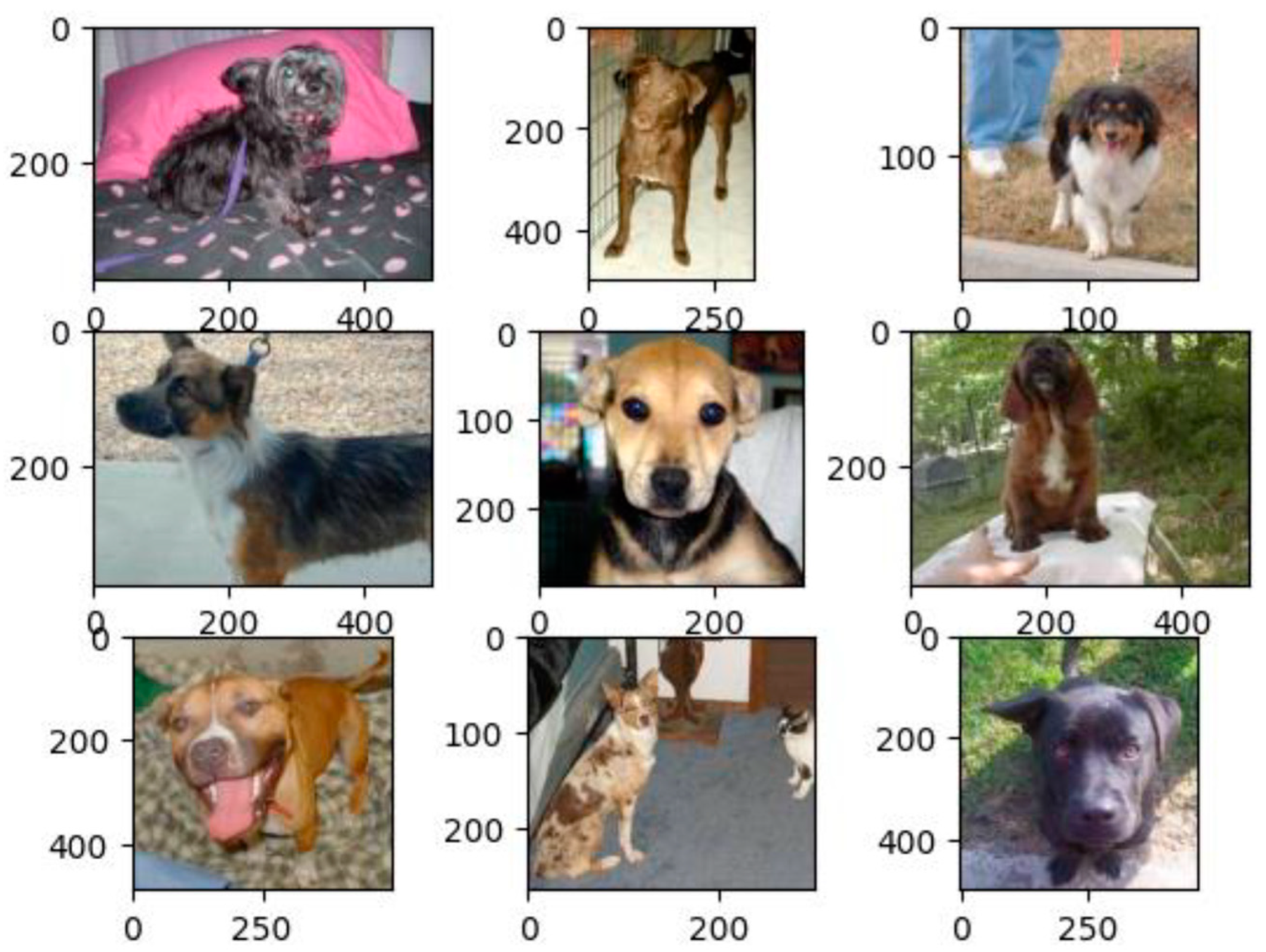
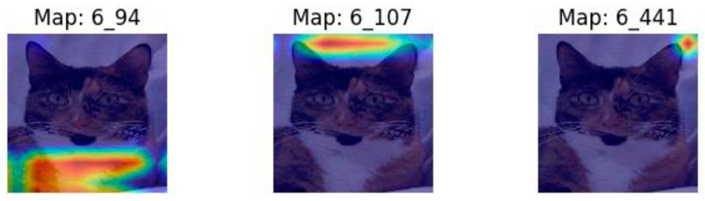
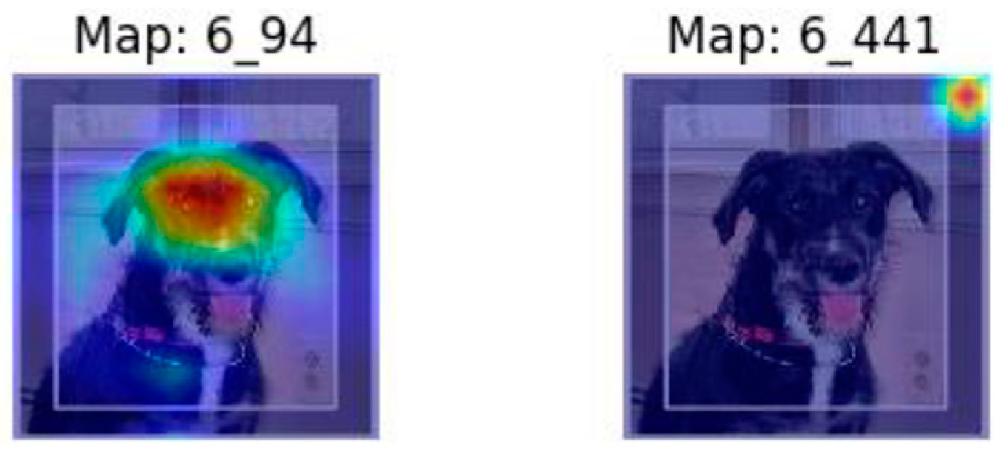
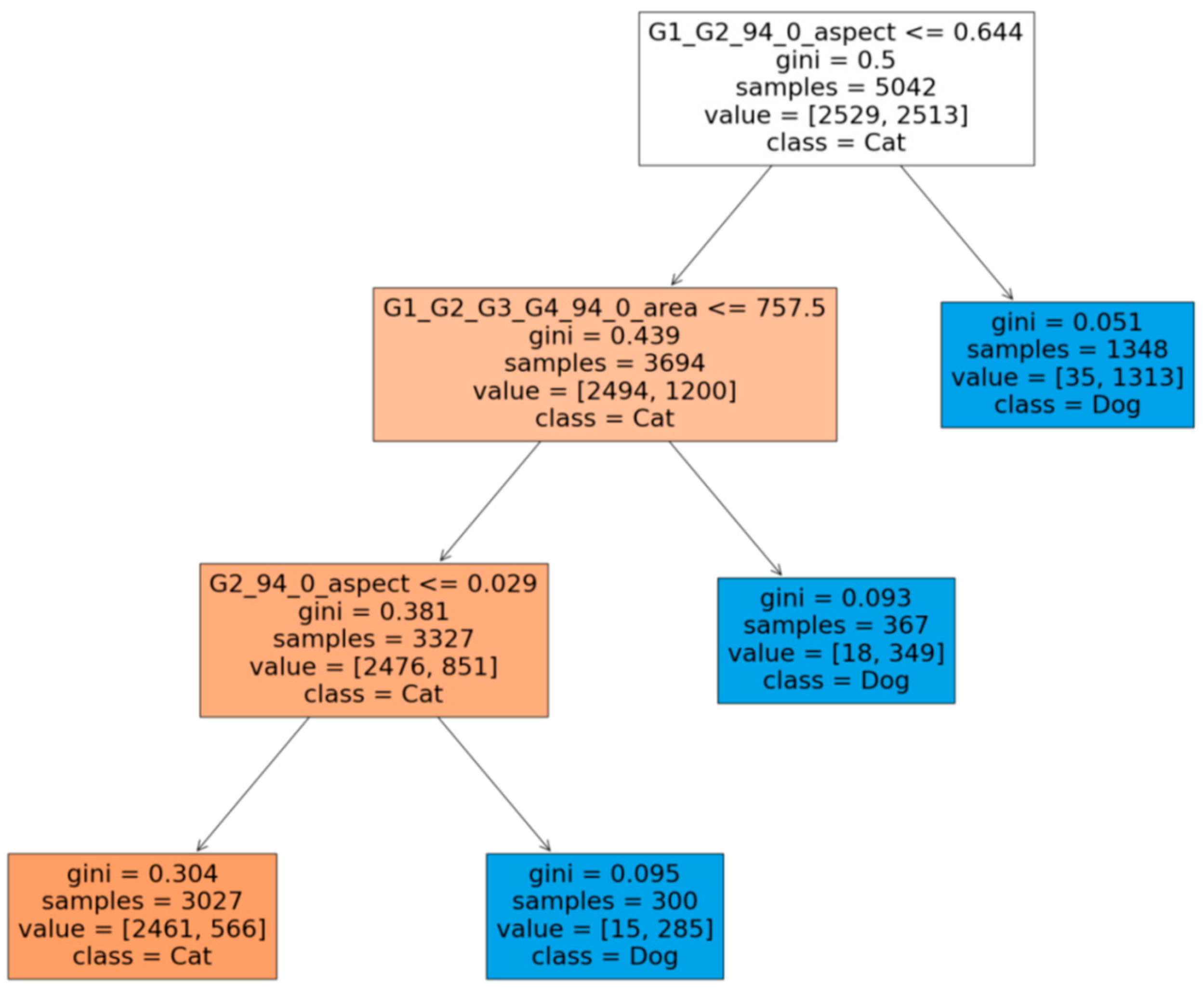
3.3.2. Cats vs. Dogs Case Study: Fine-Tuning, Feature Selection, and Image Superposition

We now present our results on the Cats vs. Dogs dataset.

Similar to the last experiment on the CelebA dataset, this experiment also followed the core methods to explain decision making from a CNN using a baseline VGG-16 with the same methodology of extracting a limited number of features. Our objective was to explain the features learned to classify cats from dogs by tracing through decision trees with grids and contours annotating features.

The dataset used for this experiment contains 25,000 images of cats and dogs, each of varying pixel size. The attribute .csv file has only two features: image_id and the label (1 = dog, 0 = cat). No filters were applied, and the whole dataset was used for training and prediction. We used 75% of the images for training and the rest for testing. Some sample images from each class are shown in Figure 10 and Figure 11.

Images were resized to the same dimension of 128 × 128 × 3, while normalization was performed by dividing the pixels’ values by 255. As with the CelebA dataset, a pretrained VGG-16 model was used for training. Compared to the CelebA dataset, this dataset presented challenges with respect to variation in the size of images, variation in the degree of rotation, and, in some cases, obfuscation of the image caused by background objects. Due to such challenges, the pretrained CNN model achieved a lower 93.1% accuracy, which fell short of the accuracy achieved on the CelebA dataset.

Samples of interpolated feature maps are shown in Figure 12 and Figure 13.

We followed the same approach as with CelebA to predict the test images and extract feature maps of dimensions 8 × 8 from the last convolution layer. We then mapped the 7 × 7 feature maps to the 128 × 128 original images using interpolation with a threshold of 95%, where the intensity of the top 5% brightest pixels was set to 255 and the rest to 0. Applying this threshold resulted in disjointed contours, similar to the last experiment.

For each contour, the area, perimeter, coordinate, and aspect ratio were computed by using coordinates (with height and width). We then translated these features to 2 × 2 grids (G1, G2, G3, G4) and changed the feature names according to the grid coordinates these contours fell in.

New feature names were represented as G2_G4_94_0_perimeter, G2_G4_94_0_area, G2_G4_94_0_aspect_ratio, and so on.

We then created a decision tree with these features with the max_depth parameter set to three, which achieved an accuracy of 87.6%, as shown in Figure 14.

Figure 14 shows that the features derived from feature map 94 dominate the classification process. In fact, all of the divisions in the tree can be attributed to this single feature map. Figure 14 also reveals that the main distinguishing characteristic between dogs and cats is the shape of the face. Dogs tend to have a long and relatively narrow face, with a larger facial area than cats. On the other hand, cats are wider while being less long (smaller height), having a more rounded appearance. Despite cats having more rounded dimensions, overall, their aspect ratio is smaller than that of dogs on account of their smaller facial area. This leads to a division at the top of the tree, where the left branch having a smaller aspect ratio for map 94 breaks in favor of cats with a probability of 3694/5042, or 73.3%, while a higher ratio favors dogs. Amongst the subpopulation of animals having a smaller aspect ratio, a larger facial area separated dogs from cats with a probability of 90.1%.

In total, a set of only three features, all derived from the same feature map, map 94, were needed for separating cats from dogs with 87.6% accuracy.

The actual rules derived from the decision tree were as follows:

• Rule-1: If face aspect ratio is >0.644 then dog, else cat.
• Rule-2: If face aspect ratio is ≤0.644 and face area is ≤757.5 then cat else dog.

The derived symbolic rules with the application of the decision tree threshold values are given below:

• Rule-1: If face aspect ratio is large then dog, else cat → capturing the vast majority of dogs.
• Rule-2: If face aspect ratio is small and face area is also small then cat, else dog → capturing the vast majority of cats but also a small fraction of dogs that happen to be small.

4. Discussion and Conclusions

With images that had a consistent orientation and distance from the camera such as with the CelebA dataset, the decision tree was able to produce high-quality human-interpretable rules with a high accuracy rate of 89.6%. This illustrates that with images that have consistent geometric properties such as orientation and size, the tree model is essentially faithful to the original CNN while producing highly interpretable decision rules.

On the other hand, with images that had large variation in orientation, distance from the camera and obfuscation (such as with cat images in the Cats vs. Dogs dataset), it was more challenging to produce human interpretable rules. Despite this, the decision tree still achieved a high accuracy rate of 87.4%. However, the aforementioned variations made it more difficult to map the features extracted from the heatmaps to physical features (head, ear, etc.), even after analysis of the image samples. Hence, we resorted to providing interpretation at the grid level, so the rules were not as easily interpretable as with the CelebA dataset. With suitable data preprocessing on the features extracted from the heatmaps, we anticipate that more interpretable rules could be produced without the use of abstract geometric grid coordinates.

In summary, the two case studies that we presented provided an interesting contrast between an environment with high-quality images with consistent geometric properties and an environment with images with a higher degree of variation in size, pose, and orientation. We observed that while the latter environment still produced rules with relatively high accuracy, the degree of interpretability of the rules produced was negatively impacted. More research is needed in such challenging environments in order to produce more interpretable features, which in turn would lead to more interpretable decision rules. One possible research direction is to investigate the application of the discrete Fourier transform on localized heatmaps to produce rotation-invariant features such as power spectrum coefficients. Such features would be rotation-invariant while preserving interpretability as they would be applied on meaningful localized areas of the original image.

We observe that both types of environments arise in real-world situations. For example, in controlled environments where images do not vary in orientation, camera distance, or angles (such as in a medical environment with X-rays, CT scans, MRI scans, passport control, etc.), our methodology can be expected to produce a similar level of high-quality human-interpretable rules as with CelebA without the need for further preprocessing methods. However, it is equally true that many environments exist, such as images captured by street cameras for law enforcement, where images have high degrees of variability in their geometric properties, so there is certainly a need for further research into methods of feature extraction. Our final thoughts on this research is that the problem is ultimately a feature selection just as with classical machine learning. The only difference here is that the features are selected not from structured tabular data but from unstructured, complex data such as images.

References

1. Russell, S.; Norvig, P. Artificial Intelligence: A Modern Approach, 4th ed.; Prentice Hall: Englewood Cliffs, NJ, USA, 2020. [Google Scholar]
2. Simonyan, K.; Zisserman, A. Very deep convolutional networks for large-scale image recognition. arXiv 2014, arXiv:1409.1556. [Google Scholar]
3. He, K.; Zhang, X.; Ren, S.; Sun, J. Deep residual learning for image recognition. In Proceedings of the IEEE Conference on Computer Vision and Pattern Recognition, Las Vegas, NV, USA, 27–30 June 2016; pp. 770–778. [Google Scholar]
4. Jia, D.; Wei, D.; Richard, S.; Li, J.L.; Kai, L.; Li, F.-F. Imagenet: A large-scale hierarchical image database. In Proceedings of the 2009 IEEE Conference on Computer Vision and Pattern Recognition, Miami, FL, USA, 20–25 June 2009; pp. 248–255. [Google Scholar]
5. Krizhevsky, A.; Hinton, G. Learning Multiple Layers of Features from Tiny Images. 2009. Available online: http://www.cs.utoronto.ca/~kriz/learning-features-2009-TR.pdf (accessed on 2 February 2024).
6. Szegedy, C.; Liu, W.; Jia, Y.; Sermanet, P.; Reed, S.; Anguelov, D.; Erhan, D.; Vanhoucke, V.; Rabinovich, A. Going deeper with convolutions. In Proceedings of the IEEE Conference on Computer Vision and Pattern Recognition, Boston, MA, USA, 7–12 June 2015; pp. 1–9. [Google Scholar]
7. Tan, M.; Le, Q. Efficientnet: Rethinking model scaling for convolutional neural networks. In Proceedings of the International Conference on Machine Learning, Long Beach, CA, USA, 9–15 June 2019; pp. 6105–6114. [Google Scholar]
8. Sandler, M.; Howard, A.; Zhu, M.; Zhmoginov, A.; Chen, L.C. Mobilenetv2: Inverted residuals and linear bottlenecks. In Proceedings of the IEEE Conference on Computer Vision and Pattern Recognition, Salt Lake City, UT, USA, 18–23 June 2018; pp. 4510–4520. [Google Scholar]
9. Castelvecchi, D. Can we open the black box of AI? Nat. News 2016, 538, 20. [Google Scholar] [CrossRef] [PubMed]
10. Das, A.; Rad, P. Opportunities and challenges in explainable artificial intelligence (xai): A survey. arXiv 2020, arXiv:2006.11371. [Google Scholar]
11. Ribeiro, M.T.; Singh, S.; Guestrin, C. “Why should I trust you? ” Explaining the predictions of any classifier. In Proceedings of the 22nd ACM SIGKDD International Conference on Knowledge Discovery and Data Mining, San Francisco, CA, USA, 13–17 August 2016; pp. 1135–1144. [Google Scholar]
12. Goodman, B.; Flaxman, S. European Union regulations on algorithmic decision-making and a “right to explanation”. AI Mag. 2017, 38, 50–57. [Google Scholar] [CrossRef]
13. Craven, M.; Shavlik, J. Extracting tree-structured representations of trained networks. Adv. Neural Inf. Process. Syst. 1995, 8, 24–30. [Google Scholar]
14. Zeiler, M.D.; Fergus, R. Visualizing and understanding convolutional networks. In Proceedings of the Computer Vision–ECCV 2014: 13th European Conference, Zurich, Switzerland, 6–12 September 2014; Proceedings of the Part I 13. Springer International Publishing: Berlin/Heidelberg, Germany, 2014; pp. 818–833. [Google Scholar]
15. Selvaraju, R.R.; Cogswell, M.; Das, A.; Vedantam, R.; Parikh, D.; Batra, D. Grad-cam: Visual explanations from deep networks via gradient-based localization. In Proceedings of the IEEE International Conference on Computer Vision, Venice, Italy, 22–29 October 2017; pp. 618–626. [Google Scholar]
16. Oh, S.J.; Schiele, B.; Fritz, M. Towards reverse-engineering black-box neural networks. In Explainable AI: Interpreting, Explaining and Visualizing Deep Learning; Springer: Cham, Switzerland, 2019; pp. 121–144. [Google Scholar]
17. Bach, S.; Binder, A.; Montavon, G.; Klauschen, F.; Müller, K.R.; Samek, W. On pixel-wise explanations for non-linear classifier decisions by layer-wise relevance propagation. PLoS ONE 2015, 10, e0130140. [Google Scholar] [CrossRef] [PubMed]
18. Achtibat, R.; Dreyer, M.; Eisenbraun, I.; Bosse, S.; Wiegand, T.; Samek, W.; Lapuschkin, S. From “where” to “what”: Towards human-understandable explanations through concept relevance propagation. arXiv 2022, arXiv:2206.03208. [Google Scholar]
19. Imagenet Dataset. Available online: https://image-net.org/ (accessed on 2 February 2024).
20. Sharma, A.K. Human Interpretable Rule Generation from Convolutional Neural Networks Using RICE: Rotation Invariant Contour Extraction. Master’s Thesis, University of North Texas, Denton Texas, TX, USA, July 2024. [Google Scholar]
21. Press, W.H.; Teukolsky, S.A.; Vetterling, W.T.; Flannery, B.P. Numerical Recipes in C: The Art of Scientific Computing, 2nd ed.; Cambridge University Press: New York, NY, USA, 1992; pp. 123–128. [Google Scholar]
22. Large-Scale CelebFaces Attributes (CelebA) Dataset. Available online: https://mmlab.ie.cuhk.edu.hk/projects/CelebA.html (accessed on 15 January 2024).
23. Kaggle Cats and Dogs Dataset. Available online: https://www.microsoft.com/en-us/download/details.aspx?id=54765&msockid=3d36009b0d73606d12a7146f0c7b6140 (accessed on 2 February 2024).
Figure 1. The feature extraction and rule generation methodology.
Information 16 00230 g001
Figure 2. The VGG-16 architecture of VGG-16. Source: uploaded by Max Ferguson at ResearchGate.
Information 16 00230 g002
Figure 3. (a) An example contour; (b) contour after 95% thresholding.
Information 16 00230 g003
Figure 4. (a) Contours before thresholding; (b) contours after 95% thresholding.
Information 16 00230 g004
Figure 5. (a) Source image for sample 6; (b) with map 106 superimposed; (c) with map 423 superimposed.
Information 16 00230 g005
Figure 6. (a) Source image for sample 6; (b) with map 106 superimposed; (c) with map 423 superimposed.
Information 16 00230 g006
Figure 7. Partitioning of contour to 2 × 2 grids G1, G2, G3 and G4 numbered left to right, top to bottom.
Information 16 00230 g007
Figure 8. Decision tree trained over derived interpretable features from the CelebA dataset.
Information 16 00230 g008
Figure 9. Eight samples from each class, capturing two feature maps and their contours from each image.
Information 16 00230 g009aInformation 16 00230 g009b
Figure 10. Sample images from the Dog class.
Information 16 00230 g010
Figure 11. Sample images from the Cat class.
Information 16 00230 g011
Figure 12. Samples from the Cat class showing feature map 6 and its contours.
Information 16 00230 g012
Figure 13. Samples from the Dog class showing feature map 6 and its contours.
Information 16 00230 g013
Figure 14. Decision tree with depth of 3 trained over the Cats vs. Dogs dataset with derived features.
Information 16 00230 g014