


A Contrastive Learning Framework for Vehicle Spatio-Temporal Trajectory Similarity in Intelligent Transportation Systems


Abstract
1. Introduction
- We propose STT-CL, a contrastive learning model for spatio-temporal trajectory computation. To the best of our knowledge, it is the first work to introduce the contrastive learning method in the study of spatio-temporal trajectory similarity.
- We innovatively introduce the concept of spatio-temporal grids and present two methods of spatio-temporal grid embedding to capture coarse-grained features.
- We design a spatio-temporal trajectory backbone encoder, namely, Spatio-Temporal Trajectory Cross-Fusion Encoder, which focuses on the correlations between coarse-grained features and fine-grained features of trajectories and fuses them into representation. It exhibits better performance for low-quality trajectories compared with previous encoders.
- We conduct extensive experiments on two real-world datasets. The experimental results illustrate that STT-CL surpasses existing baseline models in terms of performance, particularly in terms of robustness when dealing with low-quality trajectories.
2. Related Work
2.1. Spatial Trajectory Similarity
2.2. Spatio-Temporal Trajectory Similarity
2.3. Contrastive Learning for Trajectory Similarity
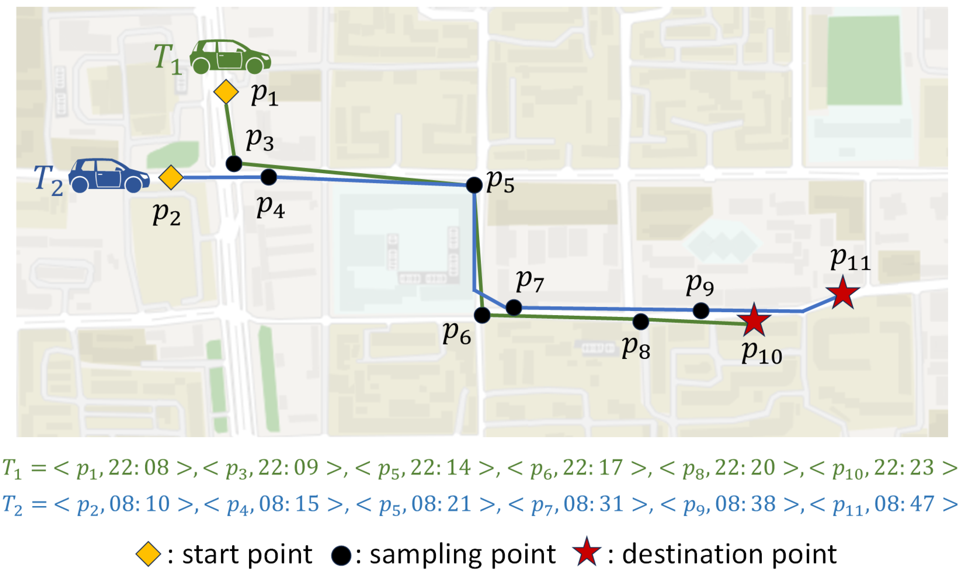
3. Preliminaries
4. The STT-CL Approach
4.1. Framework Overview
4.2. Trajectory Augmentation
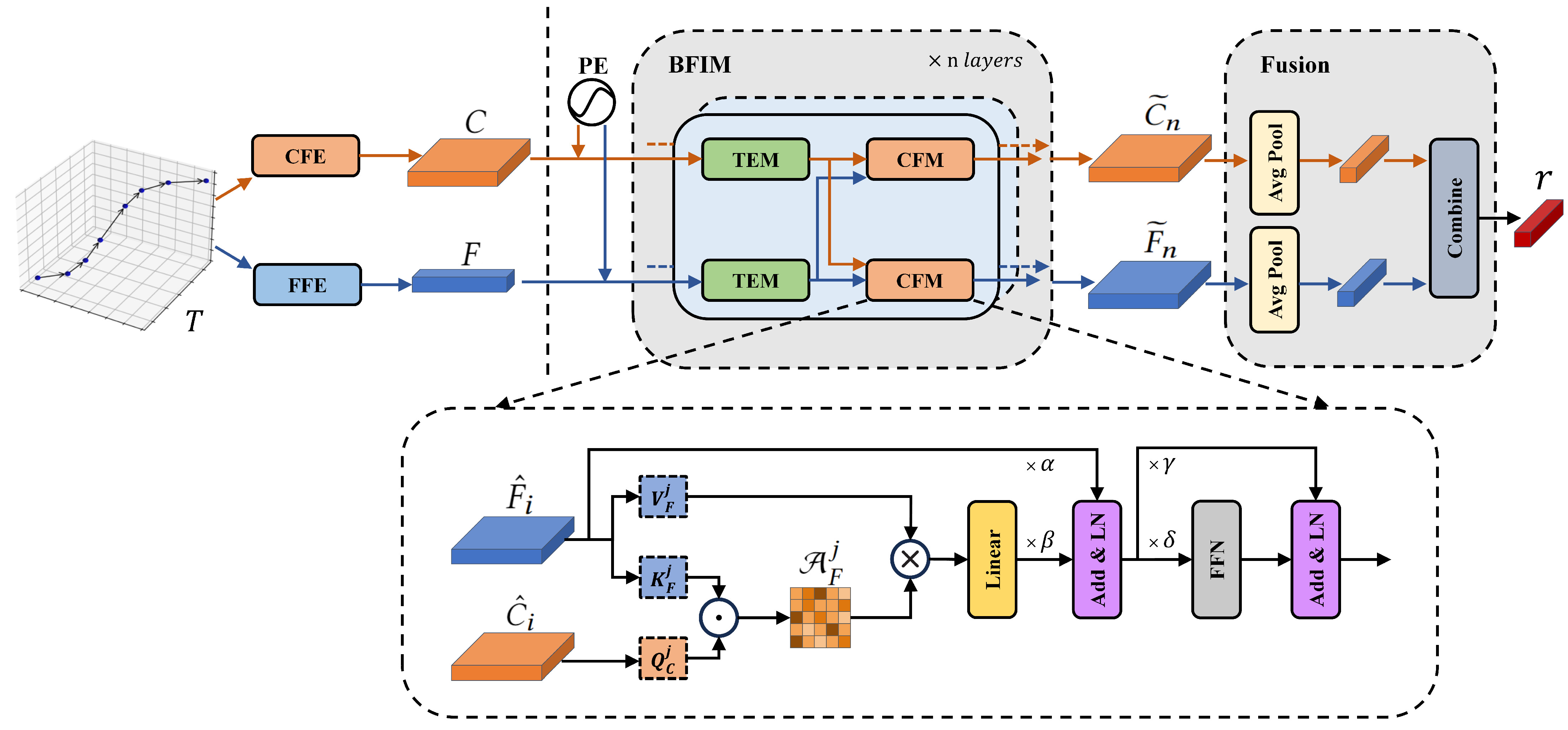
4.3. Coarse-Grained and Fine-Grained Feature Extraction
4.3.1. Coarse-Grained Feature Extraction
4.3.2. Fine-Grained Feature Extraction
4.4. Spatio-Temporal Trajectory Cross-Fusion Encoder
4.4.1. Position Encoding Section
4.4.2. BFIM Section
4.4.3. Fusion Section
4.5. STT-CL Contrastive Learning Procedure
5. Experiments
5.1. Experimental Settings
- Porto comprises 1.7 million GPS trajectory data from taxi fleets in Porto, Portugal, offering rich insights into urban mobility and traffic patterns.
5.2. Experimental Comparison
5.2.1. Effectiveness
5.2.2. Robustness
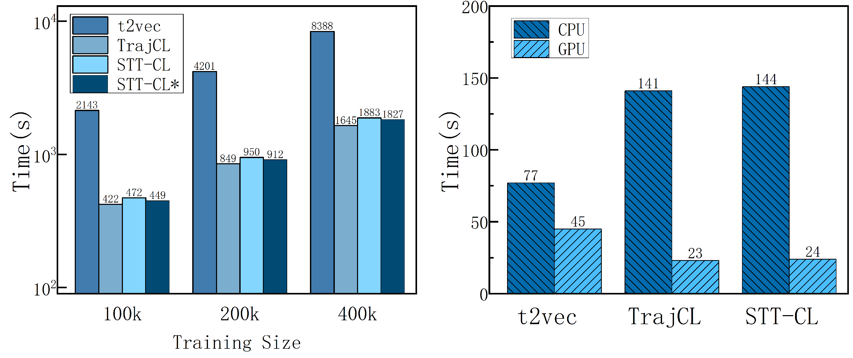
5.2.3. Efficiency
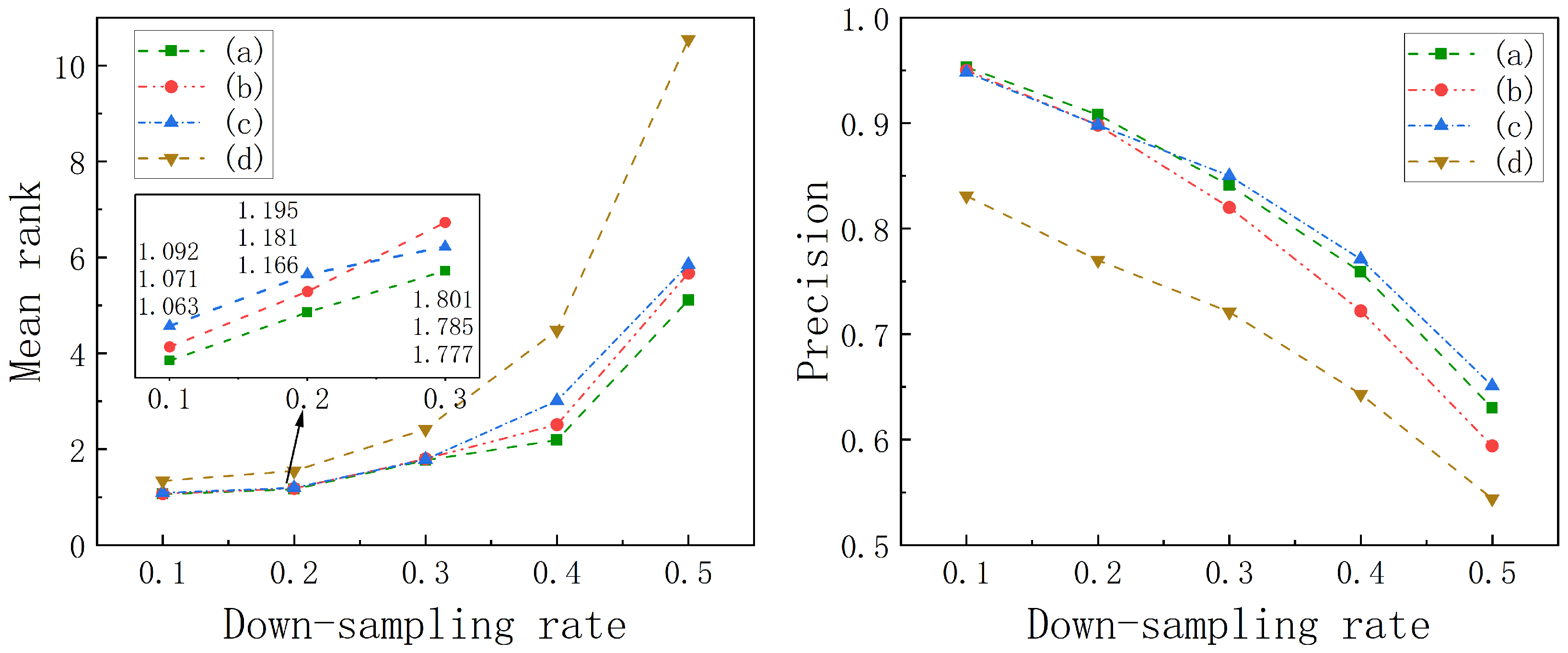
5.3. Ablation Study
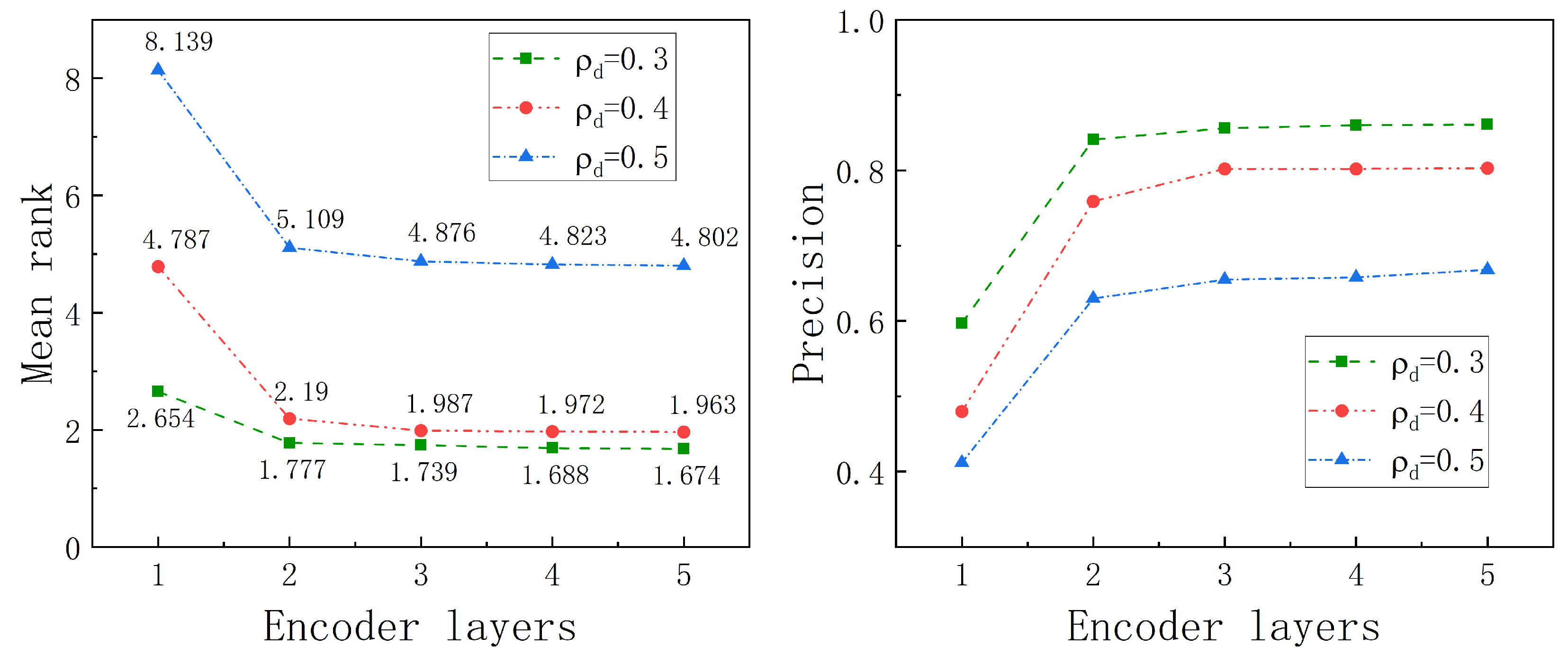
Parameter Study
6. Conclusions
Author Contributions
Funding
Institutional Review Board Statement
Informed Consent Statement
Data Availability Statement
Conflicts of Interest
References
- Zhang, H.; Ge, S.; Luo, G.; Tian, Y.; Ye, P.; Li, Y. Internet of Vehicular Intelligence: Enhancing Connectivity and Autonomy in Smart Transportation Systems. IEEE Trans. Intell. Veh. 2024, 1–5. [Google Scholar] [CrossRef]
- Cheng, X.; Duan, D.; Gao, S.; Yang, L. Integrated sensing and communications (ISAC) for vehicular communication networks (VCN). IEEE Internet Things J. 2022, 9, 23441–23451. [Google Scholar] [CrossRef]
- Amini, A.; Vaghefi, R.M.; de la Garza, J.M.; Buehrer, R.M. Improving GPS-based vehicle positioning for intelligent transportation systems. In Proceedings of the 2014 IEEE Intelligent Vehicles Symposium Proceedings, Dearborn, MI, USA, 8–11 June 2014; pp. 1023–1029. [Google Scholar]
- Jiang, Q.; Yu, L.; Ziran, D.; Shun, S. Behavior pattern mining based on spatiotemporal trajectory multidimensional information fusion. Chin. J. Aeronaut. 2023, 36, 387–399. [Google Scholar] [CrossRef]
- Glake, D.; Panse, F.; Lenfers, U.; Clemen, T.; Ritter, N. Spatio-temporal Trajectory Learning using Simulation Systems. In Proceedings of the 31st ACM International Conference on Information & Knowledge Management, Atlanta, GA, USA, 17–21 October 2022; pp. 592–602. [Google Scholar]
- Sheng, Z.; Xu, Y.; Xue, S.; Li, D. Graph-based spatial-temporal convolutional network for vehicle trajectory prediction in autonomous driving. IEEE Trans. Intell. Transp. Syst. 2022, 23, 17654–17665. [Google Scholar] [CrossRef]
- Li, L.; Erfani, S.; Chan, C.A.; Leckie, C. Multi-scale trajectory clustering to identify corridors in mobile networks. In Proceedings of the 28th ACM International Conference on Information and Knowledge Management, Beijing, China, 3–7 November 2019; pp. 2253–2256. [Google Scholar]
- Hu, D.; Chen, L.; Fang, H.; Fang, Z.; Li, T.; Gao, Y. Spatio-Temporal Trajectory Similarity Measures: A Comprehensive Survey and Quantitative Study. arXiv 2023, arXiv:2303.05012. [Google Scholar] [CrossRef]
- Chen, Y.; Yu, P.; Chen, W.; Zheng, Z.; Guo, M. Embedding-based similarity computation for massive vehicle trajectory data. IEEE Internet Things J. 2021, 9, 4650–4660. [Google Scholar] [CrossRef]
- Yi, B.K.; Jagadish, H.V.; Faloutsos, C. Efficient retrieval of similar time sequences under time warping. In Proceedings of the 14th International Conference on Data Engineering, Orlando, FL, USA, 23–27 February 1998; pp. 201–208. [Google Scholar]
- Chen, L.; Özsu, M.T.; Oria, V. Robust and fast similarity search for moving object trajectories. In Proceedings of the 2005 ACM SIGMOD International Conference on Management of Data, Baltimore, MD, USA, 14–16 June 2005; pp. 491–502. [Google Scholar]
- Alt, H. The computational geometry of comparing shapes. In Efficient Algorithms: Essays Dedicated to Kurt Mehlhorn on the Occasion of His 60th Birthday; Springer: Berlin/Heidelberg, Germany, 2009; pp. 235–248. [Google Scholar]
- Alt, H.; Godau, M. Computing the Fréchet distance between two polygonal curves. Int. J. Comput. Geom. Appl. 1995, 5, 75–91. [Google Scholar] [CrossRef]
- Li, X.; Zhao, K.; Cong, G.; Jensen, C.S.; Wei, W. Deep representation learning for trajectory similarity computation. In Proceedings of the 2018 IEEE 34th International Conference on Data Engineering (ICDE), Paris, France, 16–19 April 2018; pp. 617–628. [Google Scholar]
- Deng, L.; Zhao, Y.; Fu, Z.; Sun, H.; Liu, S.; Zheng, K. Efficient Trajectory Similarity Computation with Contrastive Learning. In Proceedings of the 31st ACM International Conference on Information & Knowledge Management, Atlanta, GA, USA, 17–21 October 2022; pp. 365–374. [Google Scholar]
- Liu, X.; Tan, X.; Guo, Y.; Chen, Y.; Zhang, Z. Cstrm: Contrastive self-supervised trajectory representation model for trajectory similarity computation. Comput. Commun. 2022, 185, 159–167. [Google Scholar] [CrossRef]
- Chen, T.; Kornblith, S.; Norouzi, M.; Hinton, G. A simple framework for contrastive learning of visual representations. In Proceedings of the International Conference on Machine Learning, Virtual, 13–18 July 2020; pp. 1597–1607. [Google Scholar]
- Gao, T.; Yao, X.; Chen, D. Simcse: Simple contrastive learning of sentence embeddings. arXiv 2021, arXiv:2104.08821. [Google Scholar]
- Yang, P.; Wang, H.; Zhang, Y.; Qin, L.; Zhang, W.; Lin, X. T3s: Effective representation learning for trajectory similarity computation. In Proceedings of the 2021 IEEE 37th International Conference on Data Engineering (ICDE), Chania, Greece, 19–22 April 2021; pp. 2183–2188. [Google Scholar]
- Feng, C.; Pan, Z.; Fang, J.; Xu, J.; Zhao, P.; Zhao, L. Aries: Accurate Metric-based Representation Learning for Fast Top-k Trajectory Similarity Query. In Proceedings of the 31st ACM International Conference on Information & Knowledge Management, Atlanta, GA, USA, 17–21 October 2022; pp. 499–508. [Google Scholar]
- Ding, J.; Zhang, B.; Wang, X.; Zhou, C. TSNE: Trajectory similarity network embedding. In Proceedings of the 30th International Conference on Advances in Geographic Information Systems, Seattle, WA, USA, 1–4 November 2022; pp. 1–4. [Google Scholar]
- Jing, Q.; Liu, S.; Fan, X.; Li, J.; Yao, D.; Wang, B.; Bi, J. Can Adversarial Training benefit Trajectory Representation? An Investigation on Robustness for Trajectory Similarity Computation. In Proceedings of the 31st ACM International Conference on Information & Knowledge Management, Atlanta, GA, USA, 17–21 October 2022; pp. 905–914. [Google Scholar]
- Shang, S.; Chen, L.; Wei, Z.; Jensen, C.S.; Zheng, K.; Kalnis, P. Trajectory similarity join in spatial networks. Proc. VLDB Endow. 2017, 10, 1178–1198. [Google Scholar] [CrossRef]
- Li, G.; Hung, C.C.; Liu, M.; Pan, L.; Peng, W.C.; Chan, S.H.G. Spatial-temporal similarity for trajectories with location noise and sporadic sampling. In Proceedings of the 2021 IEEE 37th International Conference on Data Engineering (ICDE), Chania, Greece, 19–22 April 2021; pp. 1224–1235. [Google Scholar]
- Fang, Z.; Du, Y.; Zhu, X.; Hu, D.; Chen, L.; Gao, Y.; Jensen, C.S. Spatio-temporal trajectory similarity learning in road networks. In Proceedings of the 28th ACM SIGKDD Conference on Knowledge Discovery and Data Mining, Washington, DC, USA, 14–18 August 2022; pp. 347–356. [Google Scholar]
- Zhou, S.; Han, P.; Yao, D.; Chen, L.; Zhang, X. Spatial-temporal fusion graph framework for trajectory similarity computation. World Wide Web 2023, 26, 1501–1523. [Google Scholar] [CrossRef]
- Jiang, J.; Pan, D.; Ren, H.; Jiang, X.; Li, C.; Wang, J. Self-supervised Trajectory Representation Learning with Temporal Regularities and Travel Semantics. In Proceedings of the 2023 IEEE 39th International Conference on Data Engineering (ICDE), Anaheim, CA, USA, 3–7 April 2023. [Google Scholar]
- He, K.; Fan, H.; Wu, Y.; Xie, S.; Girshick, R. Momentum contrast for unsupervised visual representation learning. In Proceedings of the IEEE/CVF Conference on Computer Vision and Pattern Recognition, Seattle, WA, USA, 14–19 June 2020; pp. 9729–9738. [Google Scholar]
- Chang, Y.; Qi, J.; Liang, Y.; Tanin, E. Contrastive Trajectory Similarity Learning with Dual-Feature Attention. In Proceedings of the 2023 IEEE 39th International Conference on Data Engineering (ICDE), Anaheim, CA, USA, 3–7 April 2023; pp. 2933–2945. [Google Scholar]
- Grill, J.B.; Strub, F.; Altché, F.; Tallec, C.; Richemond, P.; Buchatskaya, E.; Doersch, C.; Avila Pires, B.; Guo, Z.; Gheshlaghi Azar, M.; et al. Bootstrap your own latent-a new approach to self-supervised learning. Adv. Neural Inf. Process. Syst. 2020, 33, 21271–21284. [Google Scholar]
- Douglas, D.H.; Peucker, T.K. Algorithms for the reduction of the number of points required to represent a digitized line or its caricature. Cartogr. Int. J. Geogr. Inf. Geovisualization 1973, 10, 112–122. [Google Scholar] [CrossRef]
- Bojanowski, P.; Grave, E.; Joulin, A.; Mikolov, T. Enriching word vectors with subword information. Trans. Assoc. Comput. Linguist. 2017, 5, 135–146. [Google Scholar] [CrossRef]
- Vaswani, A.; Shazeer, N.; Parmar, N.; Uszkoreit, J.; Jones, L.; Gomez, A.N.; Kaiser, Ł.; Polosukhin, I. Attention is all you need. In Proceedings of the Advances in Neural Information Processing Systems 30 (NIPS 2017), Long Beach, CA, USA, 4–9 December 2017; Volume 30. [Google Scholar]
- Shen, Z.; Liu, Z.; Xing, E. Sliced recursive transformer. In Proceedings of the European Conference on Computer Vision, Tel Aviv, Israel, 23–27 October 2022; pp. 727–744. [Google Scholar]
- Liu, F.; Gao, M.; Liu, Y.; Lei, K. Self-adaptive scaling for learnable residual structure. In Proceedings of the 23rd Conference on Computational Natural Language Learning (CoNLL), Hong Kong, China, 3–4 November 2019; pp. 862–870. [Google Scholar]
- Wang, J.; Jiang, J.; Jiang, W.; Li, C.; Zhao, W.X. LibCity: An Open Library for Traffic Prediction. In Proceedings of the SIGSPATIAL/GIS, ACM, Beijing, China, 2 November 2021; pp. 145–148. [Google Scholar]
- Ranu, S.; Deepak, P.; Telang, A.D.; Deshpande, P.; Raghavan, S. Indexing and matching trajectories under inconsistent sampling rates. In Proceedings of the 2015 IEEE 31st International Conference on Data Engineering, Seoul, Republic of Korea, 13–17 April 2015; pp. 999–1010. [Google Scholar]


| Dataset | #Trajectories | #Mean Points | #Mean Length (km) |
|---|---|---|---|
| Porto 1 | 1,215,421 | 65 | 7.12 |
| BJ 2 | 846,922 | 80 | 5.26 |
| MR | Precision | ||||||||||
|---|---|---|---|---|---|---|---|---|---|---|---|
| Dataset | Method | 20 k | 40 k | 60 k | 80 k | 100 k | 20 k | 40 k | 60 k | 80 k | 100 k |
| Porto | DTW | 18.14 | 26.178 | 36.14 | 51.487 | 60.571 | 0.531 | 0.512 | 0.491 | 0.475 | 0.456 |
| EDwP | 13.75 | 15.148 | 18.154 | 21.147 | 25.442 | 0.54 | 0.521 | 0.506 | 0.498 | 0.478 | |
| Fr’echet | 10.41 | 11.154 | 15.145 | 17.245 | 19.754 | 0.597 | 0.578 | 0.561 | 0.545 | 0.52 | |
| t2vec | 1.408 | 1.892 | 2.347 | 2.777 | 3.215 | 0.839 | 0.769 | 0.729 | 0.696 | 0.67 | |
| TrajCL | 1.008 | 1.019 | 1.029 | 1.044 | 1.061 | 0.995 | 0.993 | 0.99 | 0.985 | 0.979 | |
| STT-CL | 1.008 | 1.016 | 1.022 | 1.032 | 1.036 | 0.995 | 0.993 | 0.992 | 0.988 | 0.983 | |
| p-value | 0.312 | 0.0387 | 0.0128 | 0.0116 | 0.0013 | 0.512 | 0.465 | 0.231 | 0.0735 | 0.0438 | |
| BJ | DTW | 5.15 | 7.872 | 11.157 | 16.787 | 22.145 | 0.791 | 0.771 | 0.762 | 0.748 | 0.732 |
| EDwP | 3.54 | 5.45 | 8.461 | 13.457 | 16.45 | 0.841 | 0.83 | 0.814 | 0.795 | 0.781 | |
| Fr’echet | 2.541 | 4.145 | 6.45 | 9.571 | 12.154 | 0.868 | 0.851 | 0.838 | 0.815 | 0.801 | |
| t2vec | 1.104 | 1.149 | 1.179 | 1.228 | 1.27 | 0.923 | 0.897 | 0.884 | 0.864 | 0.849 | |
| TrajCL | 1.003 | 1.003 | 1.004 | 1.007 | 1.009 | 0.997 | 0.997 | 0.996 | 0.994 | 0.994 | |
| STT-CL | 1.002 | 1.003 | 1.003 | 1.005 | 1.007 | 0.998 | 0.997 | 0.997 | 0.995 | 0.994 | |
| p-value | 0.583 | 0.653 | 0.477 | 0.407 | 0.393 | 0.654 | 0.781 | 0.541 | 0.47 | 0.487 | |
| MR | Precision | ||||||||||
|---|---|---|---|---|---|---|---|---|---|---|---|
| Dataset | Method | 0.1 | 0.2 | 0.3 | 0.4 | 0.5 | 0.1 | 0.2 | 0.3 | 0.4 | 0.5 |
| Porto | DTW | 72.148 | 110.12 | 150.215 | 200.406 | 270.587 | 0.412 | 0.354 | 0.287 | 0.254 | 0.212 |
| EDwP | 32.145 | 42.254 | 61.12 | 70.875 | 91.276 | 0.321 | 0.451 | 0.432 | 0.394 | 0.351 | |
| Fréchet | 28.124 | 51.242 | 75.45 | 125.548 | 179.412 | 0.387 | 0.341 | 0.31 | 0.281 | 0.264 | |
| t2vec | 8.763 | 26.954 | 42.572 | 79.063 | 300.898 | 0.623 | 0.549 | 0.466 | 0.395 | 0.295 | |
| TrajCL | 1.089 | 1.318 | 2.248 | 8.89 | 27.642 | 0.949 | 0.812 | 0.756 | 0.597 | 0.481 | |
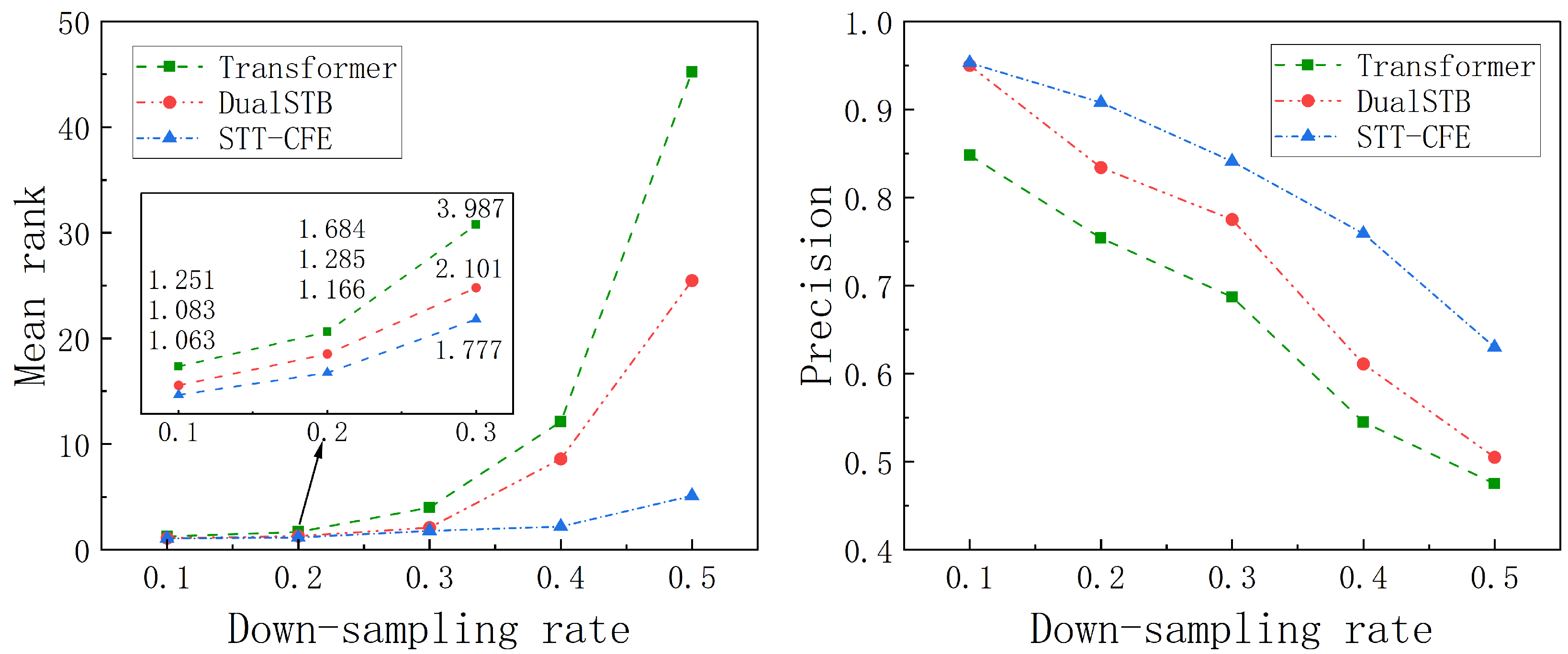
| STT-CL | 1.063 | 1.166 | 1.777 | 2.19 | 5.109 | 0.953 | 0.908 | 0.841 | 0.759 | 0.63 | |
| p-value | 0.0008 | <0.0001 | <0.0001 | <0.0001 | <0.0001 | 0.0016 | <0.0001 | <0.0001 | <0.0001 | <0.0001 | |
| BJ | DTW | 30.154 | 36.45 | 44.18 | 88.15 | 150.487 | 0.712 | 0.641 | 0.612 | 0.512 | 0.419 |
| EDwP | 18.45 | 21.109 | 22.62 | 24.375 | 30.26 | 0.725 | 0.701 | 0.687 | 0.658 | 0.635 | |
| Fréchet | 15.154 | 18.1 | 26.48 | 49.548 | 75.412 | 0.756 | 0.675 | 0.598 | 0.512 | 0.425 | |
| t2vec | 1.336 | 1.462 | 1.786 | 2.368 | 4.119 | 0.832 | 0.803 | 0.741 | 0.678 | 0.563 | |
| TrajCL | 1.021 | 1.04 | 1.098 | 1.298 | 1.87 | 0.985 | 0.97 | 0.925 | 0.865 | 0.712 | |
| STT-CL | 1.008 | 1.022 | 1.059 | 1.117 | 1.338 | 0.993 | 0.987 | 0.958 | 0.933 | 0.871 | |
| p-value | 0.0208 | 0.0093 | 0.0003 | <0.0001 | <0.0001 | 0.0411 | 0.0103 | 0.0012 | <0.0001 | <0.0001 | |
| Dataset | Method | 0.1 | 0.2 | 0.3 | 0.4 | 0.5 |
|---|---|---|---|---|---|---|
| Porto | DTW | 0.0312 | 0.0359 | 0.0398 | 0.0435 | 0.047 |
| EDwP | 0.0075 | 0.0198 | 0.0301 | 0.0358 | 0.0401 | |
| Fréchet | 0.0085 | 0.0221 | 0.033 | 0.0402 | 0.0485 | |
| t2vec | 0.0217 | 0.0266 | 0.0312 | 0.0355 | 0.0445 | |
| TrajCL | 0.0085 | 0.0132 | 0.0199 | 0.0251 | 0.0298 | |
| STT-CL | 0.012 | 0.0159 | 0.0197 | 0.0231 | 0.0287 | |
| p-value | 0.0062 | 0.0212 | 0.6328 | 0.0231 | 0.0412 | |
| BJ | DTW | 0.0236 | 0.0288 | 0.0356 | 0.0448 | 0.0497 |
| EDwP | 0.0032 | 0.0121 | 0.0188 | 0.0268 | 0.0351 | |
| Fréchet | 0.0048 | 0.0098 | 0.0189 | 0.0284 | 0.0374 | |
| t2vec | 0.0201 | 0.0216 | 0.0237 | 0.0258 | 0.0287 | |
| TrajCL | 0.0076 | 0.0089 | 0.0169 | 0.0215 | 0.0253 | |
| STT-CL | 0.0098 | 0.0121 | 0.0146 | 0.0173 | 0.0212 | |
| p-value | 0.0673 | 0.0056 | 0.0181 | <0.0001 | <0.0001 |
Disclaimer/Publisher’s Note: The statements, opinions and data contained in all publications are solely those of the individual author(s) and contributor(s) and not of MDPI and/or the editor(s). MDPI and/or the editor(s) disclaim responsibility for any injury to people or property resulting from any ideas, methods, instructions or products referred to in the content. |
© 2025 by the authors. Licensee MDPI, Basel, Switzerland. This article is an open access article distributed under the terms and conditions of the Creative Commons Attribution (CC BY) license (https://creativecommons.org/licenses/by/4.0/).
Share and Cite
Tong, Q.; Xie, Z.-C.; Ni, W.; Li, N.; Hou, S. A Contrastive Learning Framework for Vehicle Spatio-Temporal Trajectory Similarity in Intelligent Transportation Systems. Information 2025, 16, 232. https://doi.org/10.3390/info16030232
Tong Q, Xie Z-C, Ni W, Li N, Hou S. A Contrastive Learning Framework for Vehicle Spatio-Temporal Trajectory Similarity in Intelligent Transportation Systems. Information. 2025; 16(3):232. https://doi.org/10.3390/info16030232
Chicago/Turabian StyleTong, Qiang, Zhi-Chao Xie, Wei Ni, Ning Li, and Shoulu Hou. 2025. "A Contrastive Learning Framework for Vehicle Spatio-Temporal Trajectory Similarity in Intelligent Transportation Systems" Information 16, no. 3: 232. https://doi.org/10.3390/info16030232
APA StyleTong, Q., Xie, Z.-C., Ni, W., Li, N., & Hou, S. (2025). A Contrastive Learning Framework for Vehicle Spatio-Temporal Trajectory Similarity in Intelligent Transportation Systems. Information, 16(3), 232. https://doi.org/10.3390/info16030232