A Comparison of Different Transformer Models for Time Series Prediction

Abstract

Accurate estimation of the Remaining Useful Life (RUL) of lithium-ion batteries is essential for enhancing the reliability and efficiency of energy storage systems. This study explores custom deep learning models to predict RUL using a dataset from the Hawaii Natural Energy Institute (HNEI). Three approaches are investigated: an Encoder-only Transformer model, its enhancement with SimSiam transfer learning, and a CNN–Encoder hybrid model. These models leverage advanced mechanisms such as multi-head attention, robust feedforward networks, and self-supervised learning to capture complex degradation patterns in the data. Rigorous preprocessing and optimisation ensure optimal performance, reducing key metrics such as mean squared error (MSE) and mean absolute error (MAE). Experimental results demonstrated that Transformer–CNN with Noise Augmentation outperforms other methods, highlighting its potential for battery health monitoring and predictive maintenance.

1. Introduction

The growing reliance on renewable energy sources has amplified the need for advanced energy storage systems that are efficient and reliable. Lithium-ion (Li-ion) batteries have become a cornerstone of modern energy storage solutions [1], thanks to their high energy density, extended cycle life, and low self-discharge rates. These characteristics have made them integral to applications ranging from portable electronics to electric vehicles and large-scale grid storage. However, maintaining their optimal performance and extending their lifespan remain significant challenges, particularly due to the complexity of predicting their Remaining Useful Life (RUL) [2,3].

RUL is a critical metric that defines the number of cycles or durations for which a battery can function effectively before its performance degrades below an acceptable threshold. Accurate RUL prediction is essential for implementing predictive maintenance strategies, preventing unexpected failures, and enhancing the operational efficiency of energy storage systems. Traditional RUL estimation methods, such as empirical models and basic machine learning approaches, often struggle to capture the intricate and nonlinear degradation patterns exhibited by Li-ion batteries, and they have limited predictive accuracy [2].

Recent advances in deep learning, particularly Transformer models, have shown immense potential for overcoming these challenges. Originally developed for natural language processing [4], Transformers excel at handling sequential data, making them well suited for Time Series (TS) analysis required in battery health monitoring. Their self-attention mechanism enables the capture of complex dependencies and relationships within the data [5], enabling effective forecasting and feature extraction, helping them to provide a significant improvement over conventional methods.

This study explores the application of advanced transformer architectures for RUL prediction of Li-ion batteries, leveraging a dataset provided by the Hawaii Natural Energy Institute (HNEI). Initially, two primary approaches are investigated: an Encoder-only Transformer model and a CNN-Transformer hybrid model. The Encoder-only Transformer serves as a baseline for sequential modeling using self-attention. The CNN–Transformer model integrates the feature extraction capabilities of Convolutional Neural Networks (CNNs) with the temporal modeling strengths of Transformers, aiming to improve predictive accuracy. To further improve the Encoder-only Transformer, SimSiam employs a self-supervised learning approach to optimize feature space alignment between augmented views, enhancing the model’s ability to extract invariant and discriminative features from unlabeled data. This work underscores the transformative potential of Transformer-based models [6] in the prediction of RUL, paving the way for future research into their application to other battery chemistries and energy storage systems.

Data preprocessing plays a pivotal role in this research in addressing challenges such as high dimensionality, missing values, and outliers. Techniques such as normalization and sequence structuring ensure compatibility with the proposed models. The performance of these models is rigorously evaluated through extensive experiments and compared against traditional machine learning baselines.

The findings demonstrate the superior performance of both the Transformer-based and CNN–Transformer hybrid models in capturing the complex degradation patterns of Li-ion batteries. By incorporating advanced deep learning techniques, this study highlights the potential for developing next-generation battery management systems. These results contribute to improving the reliability and efficiency of energy storage technologies, with implications for a wide range of applications, including the integration of renewable energy and electric mobility.

In the next section, first the dataset used in this research is described. Then, the applied approaches are introduced. In Section 4, experimental results are demonstrated. Finally, the paper is concluded in Section 5.

2. Literature Review

Researchers have used two main approaches to predict the RUL of lithium-ion batteries: model-driven and data-driven methods [7,8]. In model-driven approaches, a mathematical model is used to predict RUL by considering the internal degradation mechanisms of the battery. However, constructing an accurate model is challenging due to the complexity of these mechanisms. Various optimization techniques, such as particle filter-based methods [9,10,11] have been employed to improve prediction accuracy. Given the involvement of multiple complex degradation processes, the accuracy of model-based approaches is limited. To address this, different recent methods such as the method using grey models [7] have been developed to enhance performance. In contrast, data-driven methods are based on the collection of historical data related to RUL. Due to the chronological and sequential nature of this data, time series processing techniques are commonly applied to improve prediction accuracy.

Several deep learning methods have demonstrated the ability to automatically learn features for TS processing. These methods are trained to extract the appropriate features using deep neural networks. For instance, in [12], stacked denoising autoencoders (SDAEs) are used to process the input data. CNN and LSTM were used to process the TS data in [13,14]. Recurrent neural network (RNN) autoencoders have been employed to extract suitable representations for TS processing [15,16,17]. Echo State Networks are also a class of deep learning methods that are used to create representations of TS that capture its dynamics [18,19,20,21]. A CNN-based structure was designed in [22] to automatically learn features that reflect the distance between a pair of TS inputs. The ability to take two TS as input increases the number of distinct instances available to train the proposed network. In [23], an Asymmetric–Symmetric Autoencoder was proposed to map scalp EEG signals to intracranial EEG, which is an expensive signal requiring an invasive and costly recording method to capture brain activity compared to EEG.

Recent studies on lithium-ion battery RUL prediction have adopted various deep learning models, with recurrent networks such as LSTM and GRU being widely applied for temporal sequence modeling [1,24]. Although effective in capturing short- and medium-term dependencies, their sequential structure limits scalability and hinders performance on long TS. CNN-based models address this by efficiently extracting local features [25], but lack the ability to capture long-range temporal relations. Transformer-based architectures have recently gained attention due to their self-attention mechanism, which enables parallel modeling of complex global dependencies [5].

In [2], a CNN–Transformer framework was developed that achieved robust state-of-health (SOH) predictions by integrating convolutional layers for local pattern extraction with self-attention for temporal dependencies. Similarly, a transferable Transformer–CNN model was introduced in [26] that demonstrated strong cross-domain generalization on NASA and CALCE datasets. Their comparative analysis also showed that this hybrid structure consistently outperformed the standalone CNN, LSTM, or Transformer baselines by leveraging complementary strengths. Building on these developments, the present study investigates three complementary directions: an Encoder-only Transformer as a baseline for sequence modeling, a CNN–Transformer hybrid to combine spatial and temporal feature learning, and a SimSiam-enhanced Transformer that incorporates self-supervised learning to improve feature invariance and adaptability across datasets.

3. Dataset

TS is a sequential collection of data that represents observations collected over time. TS analysis is crucial for applications such as forecasting, anomaly detection, and predictive modeling in various domains, including finance, healthcare, and energy. In this research, we used a TS data called RUL.

The prediction of RUL of lithium-ion batteries requires comprehensive datasets encompassing numerous charging and discharging cycles to ensure accurate model validation. This study uses the dataset provided by the Hawaii Natural Energy Institute (HNEI) [27], which offers detailed operational parameters recorded over multiple battery cycles. These parameters serve as a robust foundation for developing and validating predictive models.

The dataset, available in the repository [27], includes detailed records of these aging profiles.

The dataset utilized in this research comprises 15,064 rows and 9 features, which capture detailed operational parameters of lithium-ion batteries during their charge-discharge cycles. Key attributes include Cycle_Index, representing the sequential cycle number, discharge time (s), indicating the duration of the discharge process, and RUL (Remaining Useful Life), which specifies the remaining cycles before the end of battery life. Additional features, such as Max. Voltage Discharge (V), Min. voltage charge (V), and the time-constant current (s), provide insights into the electrical performance and temporal behavior of the battery. Figure 1 shows the first 1000 time steps of eight features for a single sample. The definition of the parameters is as follows:

• Cycle Index tracks the number of completed cycles, enabling analysis of performance degradation over time.
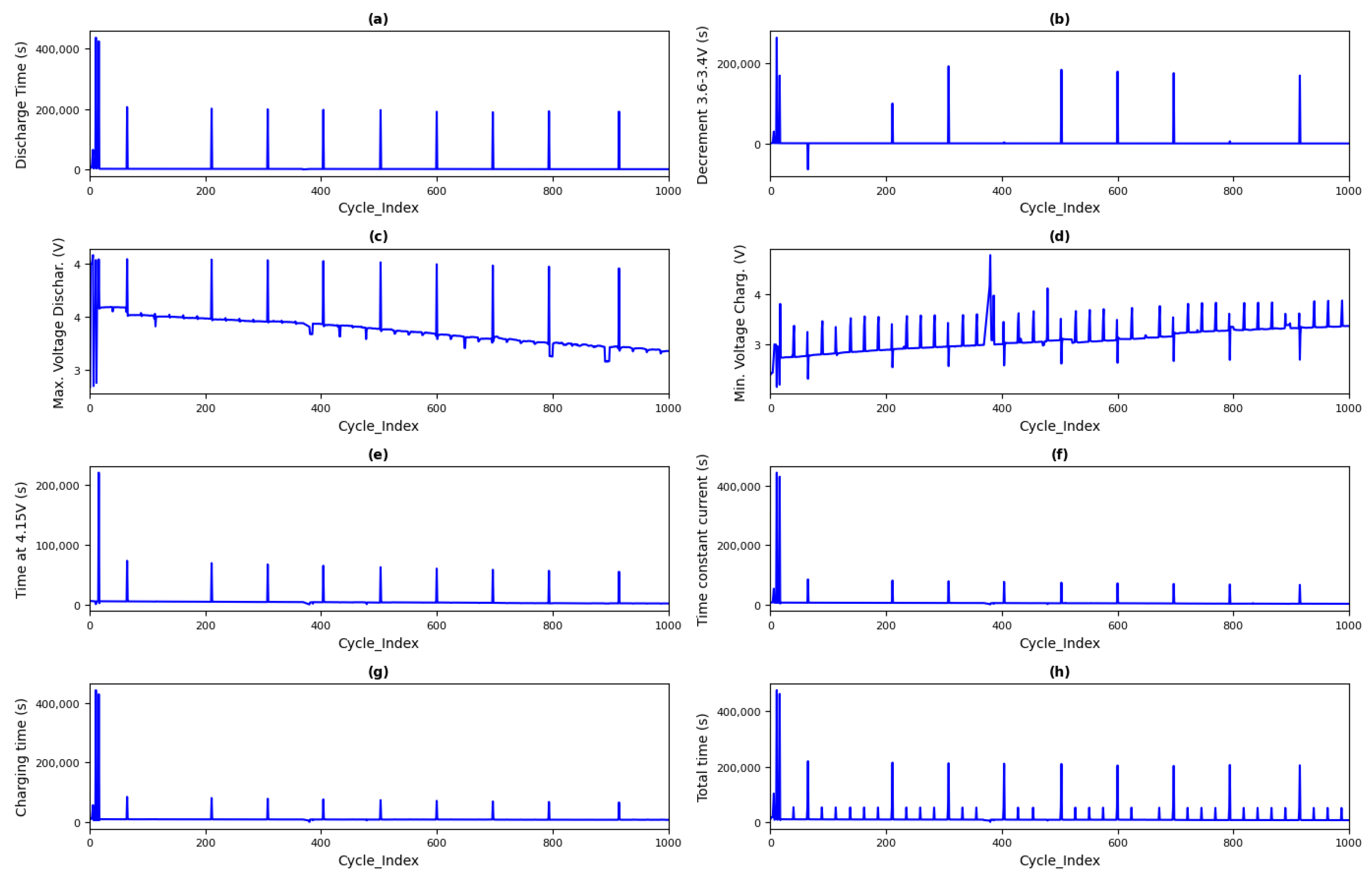
• Voltage and Current Profiles include maximum and minimum voltages during charge and discharge cycles, alongside charging durations and discharge times (Figure 1).
• Charging and Discharging Metrics detail the time spent at specific voltage levels, providing information for understanding the battery efficiency and operational behavior.

A key feature of this dataset is RUL column, which indicates the estimated number of cycles a battery can complete before its capacity falls below a threshold. This feature is derived from observed degradation patterns, which makes it invaluable for predictive maintenance and battery management strategies.

In this study, 15,064 samples are divided into training and testing sets with a ratio of 70:30. As a result

• The training set consists of 10,545 samples.
• The testing set consists of 4519 samples.

Validation data is generated during the training process using a hyperparameter tuning callback (tuner.search).

4. Applied Approaches

This study investigates three advanced deep learning approaches for predicting the RUL of lithium-ion batteries: the Encoder-only Transformer, a hybrid CNN Transformer model, and a SimSiam-based transfer learning model. Each model is designed to address specific challenges in the processing of TS data, leveraging cutting-edge architectures, and systematically optimizing training methodologies.

4.1. Data Preprocessing

Effective preprocessing ensures that the dataset is structured and normalized for efficient training, addressing variability, scaling, and sequence generation. The following steps were implemented to prepare the data for the models:

• Feature-Target Separation: The features, including sensor data such as voltage and current, were isolated from the target RUL variable to establish clear input–output relationships, as shown in

  Table 1. Separation of features and target (RUL).

  Cycle Index	Discharge Time (s)	Max. Voltage Discharge (V)	…	RUL
  1	2595.30	3.67	…	1112
  2	7408.64	4.246	…	1111
  3	7393.76	4.249	…	1110
  4	7385.50	4.250	…	1109

  where RUL is the target variable that is put in the final column.
• Scaling:

  -

  MinMax Scaling was applied to the Transformer and SimSiam models, for normalizing feature values to the range [0, 1] to ensure a uniform contribution during training.

  -

  Standard Scaling was used for the CNN–Transformer model to standardize the data with zero mean and unit variance, enhancing the functionality of the convolutional layers.

• Sequence Formation: Overlapping windows of 15 time steps were generated to capture temporal dependencies, providing context for accurate RUL predictions.
• Data Augmentation: Techniques such as Gaussian noise injection and masking were employed to simulate real-world uncertainties and improve the generalization capabilities of the models.
  Mask Augmentation: It is a data augmentation technique used in machine learning and deep learning, especially for TS data. A binary mask is generated by sampling from a Bernoulli distribution with a fixed masking probability of 0.1. This mask is applied to the input feature matrix $X\in {\mathbb{R}}^{n\times d}$, where n is the sequence length and d the number of features. A total of 10% of the values are randomly selected and replaced with zeros. The masking operation is defined in Equation (1).

  $$\tilde{X}=X\times (1-M)$$

  (1)

  where M is a binary mask matrix with the same shape as X, and the multiplication is applied element-wise. A total of 10% of the entries in M are 1.
  By simulating partial sensor dropout or data loss, the augmented dataset is created by concatenating the original and masked inputs, along with their labels, effectively doubling the training data size and improving model robustness to missing or corrupted features.
  Noise Augmentation: This technique adds Gaussian noise with a fixed standard deviation (e.g., 0.01) independently to each feature in the input sequence $X\in {\mathbb{R}}^{n\times d},$ where n is the sequence length and d the number of features. The noisy input is defined in Equation (2).

  $$\tilde{X}=X+ϵ,$$

  (2)

  where $ϵ\sim \mathcal{N}(0,{\sigma }^2)$ is a noise matrix of the same shape as X. Combining the original and augmented data increases dataset size, improving model robustness and generalization by simulating sensor noise and variability in real-world inputs.

4.2. Encoder-Only Transformer Model

The Encoder-Only Transformer model employs self-attention mechanisms to analyze sequential battery data, effectively capturing dependencies across multiple time steps [24]. Inspired by state estimation methodologies for electric vehicles, this model enhances feature extraction by leveraging its key architectural components:

• Multi-Head Attention: It facilitates simultaneous focus on various temporal segments, identifying key relationships in the data.
• Feedforward Network: It combines non-linear and linear transformations to uncover complex patterns within the input features.
• Layer Normalization and Dropout: It ensures numerical stability during training and prevents overfitting by regularizing the network.

Building on the insights from Demirci et al. [24], the Encoder-Only Transformer model demonstrates the potential of attention mechanisms to efficiently model the complex relationships present in lithium-ion battery data.

The model was optimized using the Adam optimizer, with Mean Squared Error (MSE) as the primary loss function and Mean Absolute Error (MAE) as a supplementary evaluation metric. Bayesian optimization was used to adjust the hyperparameters, ensuring optimal performance while balancing computational efficiency.

4.3. Hybrid CNN–Transformer Model

The Hybrid CNN–Transformer model combines the spatial feature extraction capabilities of Convolutional Neural Networks (CNNs) with the sequential modeling strengths of Transformers [26]. The model consists of two main components:

• CNN Component:

  -

  Convolutional Filters: Convolutional filters in CNNs extract localized patterns, such as edges, textures, or features, from the input data. These filters help identify significant trends or anomalies relevant to the task.

  -

  Global Pooling: It reduces dimensionality while preserving essential features, and ensuring compatibility with Transformer layers.

• Transformer Component: It processes extracted spatial features to capture long-term temporal dependencies using self-attention and feedforward layers.

This architecture effectively captures both local and global dependencies, making it suitable for TS tasks [25]. The model was trained using Adam Optimizer, with Bayesian search employed to optimize key hyperparameters, including the number of layers, attention heads, and learning rates.

4.4. SimSiam-Based Transfer Learning Model

The SimSiam model integrates self-supervised learning [28] with Transformers to address scenarios with limited labeled data. This approach pre-trains the model on unlabeled data before adapting it for the RUL prediction task. The methodology includes the following:

• Pre-Training: The model learns to match feature representations from different augmented views of the same sequence, encouraging invariance to minor perturbations.
• Cosine Similarity Loss: This loss function guides the pretraining process by maximizing the similarity between paired feature representations while avoiding trivial solutions through gradient control mechanisms.

The results of the pretrained stage is a backbone model pretrained on unlabelled data. After pretraining, the SimSiam model is reconfigured and trained on labelled RUL data to align its learned features with task-specific requirements, ensuring robust and accurate predictions.

The reconfiguration process includes two distinct approaches regarding the backbone model in the Transformer model:

• Untrainable Backbone: In this configuration, the backbone model remains frozen (untrainable) during the second phase of training. This allows the pre-trained features to remain intact, with the additional layers adapting these features to the RUL prediction task. This approach reduces the risk of overfitting, but may limit the model’s ability to adapt to task-specific details in the labelled data.
• Trainable Backbone: In this configuration, the layers in the backbone model are made trainable during the second phase of training (Supervised training phase). This allows the pre-trained features to be fine-tuned for the RUL prediction task, enhancing the model’s adaptability and alignment with the specific dataset. However, it also introduces a greater risk of overfitting if not managed with care.

These two configurations were evaluated to understand the impact of freezing or fine-tuning the backbone model on the final model’s performance. The results demonstrated that making the backbone trainable led to a better alignment of the learned features with task-specific requirements, resulting in more accurate RUL predictions.

4.5. Hyperparameter Tuning

Hyperparameter tuning is the process of optimizing the hyperparameters of a machine learning model, such as learning rates, batch sizes, and network architectures. Proper tuning ensures improved model performance and avoids overfitting or underfitting.

The hyperparameters were systematically tuned using Keras Tuner and Bayesian optimization, ensuring a balance between model performance and computational feasibility. Key hyperparameters included the following:

• Attention Heads: Explored between 2 and 8 to capture diverse feature subspaces without excessive computational costs.
• Feedforward Dimensions: Tuned between 128 and 512 units to balance the model’s learning capacity with the risk of overfitting.
• Dropout Rates: Adjusted between 0.01 and 0.3 to enhance generalization while retaining critical features.
• Learning Rates: Evaluated on a logarithmic scale from $1\times {10}^{-4}$ to $1\times {10}^{-2}$ to ensure efficient convergence during training.
• Transformer Layers (Hybrid Model): Limited to 1 to 4 layers to capture long-range dependencies while maintaining computational efficiency.

These hyperparameters were optimized to minimize validation loss and maximize accuracy, with Bayesian optimization providing an efficient exploration strategy to identify the best configurations for the models.

4.6. Theoretical and Mathematical Framework

In this section, the theoretical backgrounds of the Encoder-only Transformer, and Transformer–CNN models are described using mathematical equations to clarify the applied models.

4.6.1. Theoretical Background of the Encoder-Only Transformer Model

The Encoder-only Transformer captures temporal dependencies in battery sequences through self-attention mechanism, which evaluates relationships between all positions simultaneously, inspired by the original transformer model [4]. It contains a multi-head attention module that consists of multiple self-attention blocks. Each self-attention block creates three vectors called query, key, and value using three different linear layers. A dot product is used to compare the query with the key to calculate the attention weights, as shown in Equation (3).

$$A=\mathrm{softmax}\left({\displaystyle \frac{Q{K}^{\top }}{\sqrt{d_k}}}\right)$$

(3)

where Q, K, V are query, key, and value matrices. $dk$ is the dimension of each row in Q, and K. This formulation enables the model to highlight the most informative features while down-weighting irrelevant signals effectively. The generated attention is multiplied by V to generate the output of the multi-head attention module.

Stability during training is achieved by combining residual connections, dropout, and normalization together, expressed in Equation (4).

$$X^{\prime }=\mathrm{LayerNorm}(X+\mathrm{Dropout}\left(\mathrm{MHA}\left(X\right)\right))$$

(4)

where $MHA(.)$ is the multi-head attention block.

4.6.2. Theoretical Background of the Transformer–CNN Model

To complement global self-attention with localized feature extraction, convolutional layers are incorporated before the Transformer encoder [2]. In this research, local patterns are captured using Equation (5).

$$U=\mathrm{Conv}1\mathrm{D}(X;C,k)$$

(5)

where C represents the number of filters and k denotes the chosen kernel size. The feature maps are then reduced with global average pooling across all time steps using Equation (6).

$$g={\displaystyle \frac{1}{T^{\prime }}}\sum U[:,t,:]$$

(6)

where $T^{\prime }$ is the total number of time steps in each sample in U, which is a convolved form of a batch of the input time series X. This pooled representation is subsequently repeated along the time axis to reconstruct a sequence input for the Transformer as shown in Equation (7).

$$S=\mathrm{repeat}(g,T)$$

(7)

By combining convolutional layers for capturing short-term patterns with self attention for long-range dependencies, this hybrid design effectively models both fine-grained fluctuations and overall battery degradation trends [26].

5. Experimental Results

The experimental evaluation of Encoder-Only Transformer, and CNN–Transformer hybrid models without any augmentation and with two augmentation methods, and SimSiam Transfer Learning was conducted to assess their effectiveness in predicting the Remaining Useful Life (RUL) of lithium-ion batteries. The models were evaluated using metrics such as Mean Absolute Error (MAE), Mean Squared Error (MSE), and validation loss. Visual comparisons between predicted and actual RUL values further highlighted their performance.

5.1. Evaluation Metrics

The performance of the models was measured using the following metrics:

• Mean Absolute Error (MAE): Measures the average magnitude of errors in predictions. Lower MAE indicates better accuracy.

  $$\mathrm{MAE}={\displaystyle \frac{1}{n}}\sum _{i=1}^n\left|y_i-{\widehat{y}}_i\right|$$

  (8)

  where n is the number of observations, $y_i$ is the actual value and ${\widehat{y}}_i$ is the predicted value.
• Mean Squared Error (MSE): Focuses on the average squared differences between predicted and actual values. It is sensitive to larger errors.

  $$\mathrm{MSE}={\displaystyle \frac{1}{n}}\sum _{i=1}^n{\left(y_i-{\widehat{y}}_i\right)}^2$$

  (9)
  The same metric was used as Validation Loss to quantify the model’s ability to generalize during training.
• Coefficient of Determination ($R^2$): Represents the proportion of variance in the target variable explained by the model, with values closer to 1 indicating a better fit.

  $$R^2=1-{\displaystyle \frac{{\sum }_{i=1}^n{\left(y_i-{\widehat{y}}_i\right)}^2}{{\sum }_{i=1}^n{\left(y_i-\overline{y}\right)}^2}}$$

  (10)

5.2. Results of the Encoder-Only Transformer Model

The Encoder-Only Transformer model was trained for 200 epochs. The final training and validation losses (MSE) were 47.07 and 41.07, respectively, as seen in Figure 2. The MAE for training was 4.51, while the validation MAE was 3.99. Based on the results shown in the figure, the validation loss is lower than the training loss. This indicates that the model has good generalization ability and is not overfitting. One possible reason for this is the use of a single Transformer encoder layer, which significantly reduces the number of training parameters compared to models with multiple Transformer layers. Fewer parameters can limit the model’s capability to overfit the training data, which may explain the relatively high training loss observed in Figure 2. However, this also contributes to a comparatively low validation loss, as the model remains less complex and more generalizable. The predicted vs. actual RUL bar chart for a number of samples, shown in Figure 3, demonstrates the alignment of the model with the actual values. Detailed numerical results for selected test samples are shown in

Table 2. Numerical predictions vs. actual values for the encoder-only Transformer model.

Sample	Actual RUL	Predicted RUL
1	63.00	63.89
2	874.00	879.69
3	891.00	891.67
4	301.00	296.32
5	345.00	342.22

.

5.3. Results of the Transformer–CNN Hybrid Model Without Augmentation

The Transformer–CNN hybrid model without augmentation yielded comparatively lower performance metrics than the augmented models. After 200 epochs, the training loss was 4.12, and the validation loss reached 9.78. The MAE for training was 1.87, while the MAE for validation was 2.34, indicating less accurate predictions compared to the augmented approaches.

5.4. Results of the Transformer-CNN with Mask Augmentation

The Transformer-CNN model with mask augmentation demonstrated strong performance after 200 training epochs. The final training and validation losses were 3.28 and 8.41, respectively, as shown in Figure 4. The MAE for training was 1.34, and the validation MAE was 1.75. Training loss stabilized after epoch 100 while validation loss increased slightly beyond epoch 150 indicating moderate overfitting. Performance remained robust due to mask augmentation applied to all input features at a %1 probability. This augmentation was implemented by randomly masking elements of the input features which increased the diversity of inputs and reduced the model’s reliance on specific local patterns, thereby improving generalization across varying battery operating conditions.

5.5. Results of the Transformer–CNN Hybrid Model with Noise Augmentation

The Transformer–CNN model with noise augmentation achieved the best results among the models. After 200 training epochs, training and validation losses were 3.19 and 3.85, as shown in Figure 5. The training MAE was 1.33, and the validation MAE was 1.39. The loss curves are closely aligned and plateaued around epoch 150, indicating strong convergence and no overfiting. The small gap between training and validation metrics confirms well performed generalization, due to noise augmentation introducing realistic variability that helps the model adapt to unseen conditions.

A comparison of Figure 2 and Figure 5 shows that the Transformer–CNN hybrid model with noise augmentation demonstrates better learning performance than the Encoder-Only Transformer model. As shown in Figure 2, the training and validation losses stop decreasing significantly and reach a near-constant level around a higher loss range (40–50), stabilizing after approximately 100 epochs. In contrast, in Figure 5, the losses converge within a much lower range (below 5) and gradually flatten after 150 epochs. In Figure 4, the training and validation losses reach a range below 15 after 150 epochs, showing better convergence compared to Figure 2.

Table 3. Comparison of hybrid model performance with and without augmentation.

Model	Loss (MSE)	MAE	R2 Score
Transformer–CNN (Without Augmentation)	9.78	2.34	0.99985
Transformer–CNN (Mask Augmentation)	4.31	1.39	0.999958
Transformer–CNN (Noise Augmentation)	3.47	1.22	0.999966

compares different metrics for Transformer–CNN, Transformer–CNN with mask augmentation, and Transformer–CNN with noise augmentation. The results show that Transformer–CNN with noise augmentation has the best performance. It has the minimum error, and it also has the maximum $R^2$ value.

5.6. Results of the SimSiam Transfer Learning Model

The SimSiam Transfer Learning model was evaluated using two configurations:

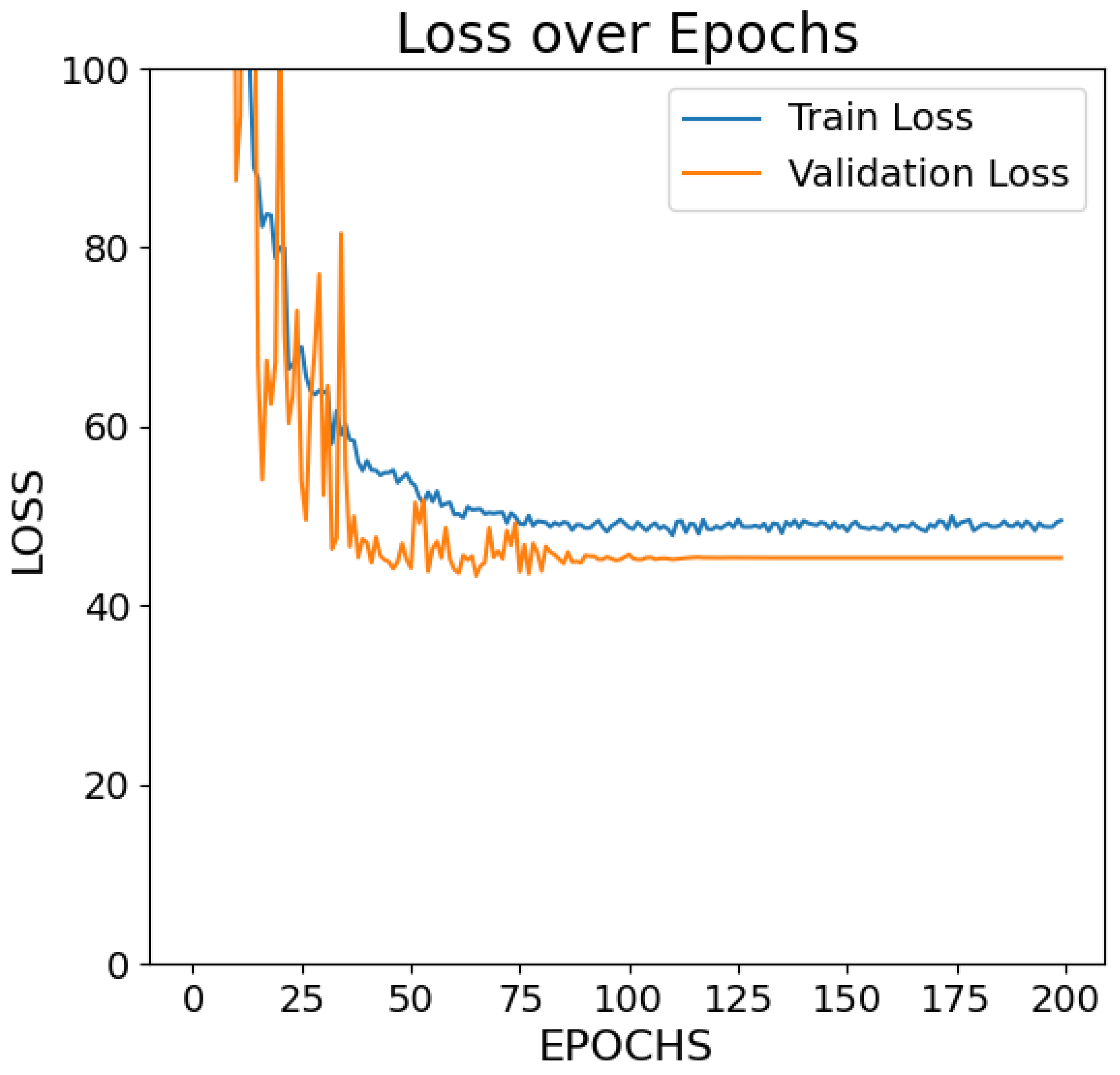
• Untrainable backbone model: The backbone remained untrainable during the second phase of training. Training and validation losses were 903.54 and 716.93, respectively, with MAE values of 19.90 and 16.35. Significant deviations in the predicted versus actual RUL highlight the model’s limitations.
• Adaptable backbone model: In this configuration, the backbone layer of the SimSiam model was allowed to adjust during the second training phase. Training and validation losses reduced to 80.63 and 51.53, respectively, with MAE values of 6.62 and 4.96. Detailed numerical results are provided in the last row of

  Table 4. Performance metrics for all models on the test set.

  Model	Loss (MSE)	MAE	R2 Score
  Encoder-Only Transformer	41.07	3.99	0.99960
  Transformer–CNN (Without Aug.)	9.78	2.34	0.99985
  Transformer–CNN (Mask Aug.)	4.31	1.39	0.99996
  Transformer–CNN (Noise Aug.)	3.47	1.22	0.99997
  SimSiam Transfer Learning (Untrainable)	716.93	16.35	0.99020
  SimSiam Transfer Learning (Adaptable)	51.53	4.96	0.99910

  .
  Table 5. Best performing hyperparameters for all applied methods.

  Model	Number of Heads	Feed Forward Network Dimensionality (dff)	Dropout Rate	Learning Rate
  Encoder-Only Transformer	2	512	0.01	0.00103
  Transformer–CNN (Without Aug.)	2	256	0.01	0.00045
  Transformer–CNN (Mask Aug.)	2	384	0.01	0.00075
  Transformer–CNN (Noise Aug.)	2	256	0.01	0.00055
  SimSiam Transfer Learning (Untrainable)	4	512	0.02	0.04500
  SimSiam Transfer Learning (Adaptable)	4	512	0.02	0.01500

  shows the best values for the hyperparameters of different models. An additional hyperparameter, Number of Layers, was tuned exclusively for the Transformer–CNN models. It defines the number of Transformer encoder layers in the architecture and was not applicable to the Encoder-Only Transformer or SimSiam Transfer Learning models.

The performance metrics of the test set for all models are summarized in Table 4. The Transformer–CNN with Noise Augmentation exhibited the most accurate predictions and the lowest errors, achieving an MSE of 3.47, an MAE of 1.22, and an R² score of 0.99997. This model outperformed the others, highlighting its robustness and effectiveness in RUL prediction. No other model achieved such high levels of accuracy and precision in evaluating this dataset.

6. Conclusions

This study evaluated the effectiveness of Transformer-based models in predicting the RUL of lithium-ion batteries. Different Transformer methods including CNN–Encoder-Only Transformer, Encoder-Only Transformer, and SimSiam Transfer were tested. These models leverage advanced mechanisms, including multi-head attention and feedforward networks, to capture complex temporal dependencies and data patterns. Rigorous data preprocessing, hyperparameter optimization, and incorporation of dropout regularization and layer normalization were pivotal in enhancing model performance and preventing overfitting.

The proposed transformer-based models are well suited for integration into real-world battery management systems (BMS) in electrical vehicles, renewable energy storage, and industrial power units. They enable real-time RUL prediction, support condition-based maintenance, and reduce unexpected failures. The models can be optimized using frameworks like TensorFlow Lite or ONNX for on-device deployment, allowing efficient inference on embedded hardware with limited resources.

While this study demonstrates the effectiveness of transformer-based models on the HNEI dataset (NMC-LCO 18650 cells), we acknowledge that the dataset does not capture other battery chemistries and form factors. This represents a limitation of the current work. Evaluating the proposed models on modern datasets to further assess their generalizability to contemporary battery technologies is an important direction for future research.

Although the HNEI dataset provides realistic operational conditions with dynamic load cycles and variations in ambient temperature, the scope remains limited to a specific battery chemistry and manufacturer. Future work should explore model generalization across other publicly available datasets, such as NASA or CALCE, and investigate robustness to previously unseen chemistries (e.g., LFP, NMC), form factors (e.g., pouch, prismatic), and extreme environmental conditions.

In conclusion, this research establishes a strong foundation for applying Transformer models in predictive maintenance, and it improves the RUL prediction accuracy. This contributes to more reliable, and sustainable energy storage solutions. These advancements support the global transition to renewable energy and electric mobility.

References

- Adithya, C.H.; Hegde, A.R.; Prasad, S. Early Prediction of Remaining Useful Life for Li-ion Batteries Using Transformer Model with Dual Auto-Encoder and Ensemble Techniques. In Proceedings of the 2024 IEEE 9th International Conference for Convergence in Technology (I2CT), Pune, India, 5–7 August 2024; IEEE: New York, NY, USA, 2024; pp. 1–7. [Google Scholar]
- Gu, X.; See, K.W.; Li, P.; Shan, K.; Wang, Y.; Zhao, L.; Lim, K.C.; Zhang, N. A novel state-of-health estimation for the lithium-ion battery using a convolutional neural network and transformer model. Energy 2023, 262, 125501. [Google Scholar] [CrossRef]
- Demirci, O.; Taskin, S.; Schaltz, E.; Demirci, B.A. Review of battery state estimation methods for electric vehicles-Part II: SOH estimation. J. Energy Storage 2024, 96, 112703. [Google Scholar] [CrossRef]
- Vaswani, A.; Shazeer, N.; Parmar, N.; Uszkoreit, J.; Jones, L.; Gomez, A.N.; Kaiser, L.; Polosukhin, I. Attention is all you need. arXiv 2017, arXiv:1706.03762. [Google Scholar]
- Song, W.; Wu, D.; Shen, W.; Boulet, B. A remaining useful life prediction method for lithium-ion battery based on temporal transformer network. Procedia Comput. Sci. 2023, 217, 1830–1838. [Google Scholar] [CrossRef]
- Kim, G.; Choi, J.G.; Lim, S. Using transformer and a reweighting technique to develop a remaining useful life estimation method for turbofan engines. Eng. Appl. Artif. Intell. 2024, 133, 108475. [Google Scholar] [CrossRef]
- Wang, S.; Li, Y.; Zhou, S.; Chen, L.; Michael, P. Remaining useful life prediction of lithium-ion batteries using a novel particle flow filter framework with grey model. Sci. Rep. 2025, 15, 3311. [Google Scholar] [CrossRef] [PubMed]
- Jiao, R.; Peng, K.; Dong, J. Remaining useful life prediction of lithium-ion batteries based on conditional variational autoencoders-particle filter. IEEE Trans. Instrum. Meas. 2020, 69, 8831–8843. [Google Scholar] [CrossRef]
- Miao, Q.; Xie, L.; Cui, H.; Liang, W.; Pecht, M. Remaining Useful Life Prediction of Lithium-Ion Battery with Unscented Particle Filter Technique. Microelectron. Reliab. 2013, 53, 805–810. [Google Scholar] [CrossRef]
- Qiu, X.; Wu, W.; Wang, S. Remaining Useful Life Prediction of Lithium-Ion Battery Based on Improved Cuckoo Search Particle Filter and a Novel State of Charge Estimation Method. J. Power Sources 2020, 450, 227700. [Google Scholar] [CrossRef]
- Wang, S.; Han, W.; Chen, L.; Zhang, X.; Pecht, M. Experimental Verification of Lithium-Ion Battery Prognostics Based on an Interacting Multiple Model Particle Filter. Trans. Inst. Meas. Control 2020, 42, 01423312. [Google Scholar] [CrossRef]
- Hu, Q.; Zhang, R.; Zhou, Y. Transfer learning for short-term wind speed prediction with deep neural networks. Renew. Energy 2016, 85, 83–95. [Google Scholar] [CrossRef]
- Taherkhani, A.; Cosma, G.; Alani, A.A.; McGinnity, T.M. Activity Recognition from Multi-modal Sensor Data Using a Deep Convolutional Neural Network. In Intelligent Computing; SAI 2018; Advances in Intelligent Systems and Computing; Arai, K., Kapoor, S., Bhatia, R., Eds.; Springer: Cham, Switzerland, 2019; Volume 857. [Google Scholar] [CrossRef]
- Fulsunder, S.; Umar, S.; Taherkhani, A.; Liu, C.; Yang, S. Hand Gesture Recognition Using a Multi-modal Deep Neural Network. In Intelligent Information Processing XII; IIP 2024; IFIP Advances in Information and Communication Technology; Shi, Z., Torresen, J., Yang, S., Eds.; Springer: Cham, Switzerland, 2024; Volume 704. [Google Scholar] [CrossRef]
- Malhotra, P.; Vig, L.; Agarwal, P.; Shroff, G. TimeNet: Pre-trained deep recurrent neural network for time series classification. In Proceedings of the 25th European Symposium on Artificial Neural Networks, Computational Intelligence and Machine Learning, Bruges, Belgium, 26–28 April 2017. [Google Scholar]
- Mehdiyev, N.; Lahann, J.; Emrich, A.; Enke, D.; Fettke, P.; Loos, P. ScienceDirect ScienceDirect time series classification using deep learning for process planning: A case from the process industry. Proc. Comput. Sci. 2017, 114, 242–249. [Google Scholar] [CrossRef]
- Rajan, D.; Thiagarajan, J.J. A Generative Modeling Approach to Limited Channel ECG Classification. In Proceedings of the 40th Annual International Conference of the IEEE Engineering in Medicine and Biology Society (EMBC), Honolulu, HI, USA, 18–21 July 2018; pp. 2571–2574. [Google Scholar]
- Aswolinskiy, W.; Reinhart, R.F.; Steil, J. Time series classification in reservoir- and model-space: A comparison. In Artificial Neural Networks in Pattern Recognition; Schwenker, F., Abbas, H.M., El Gayar, N., Trentin, E., Eds.; Springer International Publishing: Cham, Switzerland, 2016; pp. 197–208. [Google Scholar]
- Bianchi, F.M.; Scardapane, S.; Jenssen, R. Reservoir computing approaches for representation and classification of multivariate time series. arXiv 2018, arXiv:1803.07870. [Google Scholar] [CrossRef] [PubMed]
- Chouikhi, N.; Ammar, B.; Alimi, A.M.; Member, S. Genesis of basic and multi-layer echo state network recurrent autoencoder for efficient data representations. arXiv 2018, arXiv:1804.08996. [Google Scholar] [CrossRef]
- Ma, Q.; Shen, L.; Chen, W.; Wang, J.; Wei, J.; Yu, Z. Functional echo state network for time series classification. Inf. Sci. 2016, 373, 1–20. [Google Scholar] [CrossRef]
- Taherkhani, A.; Cosma, G.; McGinnity, T.M. A Deep Convolutional Neural Network for Time Series Classification with Intermediate Targets. SN Comput. Sci. 2023, 4, 832. [Google Scholar] [CrossRef]
- Antoniades, A.; Spyrou, L.; Martin-Lopez, D.; Valentin, A.; Alarcon, G.; Sanei, S.; Took, C.C. Detection of interictal discharges with convolutional neural networks using discrete ordered multichannel intracranial EEG. IEEE Trans. Neural Syst. Rehabil. Eng. 2017, 4320, 1–10. [Google Scholar] [CrossRef] [PubMed]
- Chen, D.; Hong, W.; Zhou, X. Transformer network for remaining useful life prediction of lithium-ion batteries. IEEE Access 2022, 10, 19621–19628. [Google Scholar] [CrossRef]
- Costa, N.; Sánchez, L.; Anseán, D.; Dubarry, M. Li-ion battery degradation modes diagnosis via Convolutional Neural Networks. J. Energy Storage 2022, 55, 105558. [Google Scholar] [CrossRef]
- Gui, X.; Du, J.; Song, L.; Yan, Z.; Guo, L. A Transformer-CNN Based Transferable Model for State-of-Health Prediction of Lithium-ion Batteries. In Proceedings of the 2023 Global Reliability and Prognostics and Health Management Conference (PHM-Hangzhou), Hangzhou, China, 12–15 October 2023; IEEE: New York, NY, USA, 2023; pp. 1–8. [Google Scholar]
- GitHub. Battery RUL Prediction Dataset. Available online: https://github.com/ignavinuales/Battery_RUL_Prediction/blob/main/Datasets/HNEI_Processed/Final%20Database.csv (accessed on 7 August 2025).
- Chen, X.; He, K. Exploring simple siamese representation learning. In Proceedings of the IEEE/CVF Conference on Computer Vision and Pattern Recognition, Nashville, TN, USA, 20–25 June 2021; pp. 15750–15758. [Google Scholar]