CLARE: Context-Aware, Interactive Knowledge Graph Construction from Transcripts

Abstract

Knowledge graphs (KGs) represent a promising approach for detecting and correcting errors in automated audio and video transcripts. Yet the lack of accessible tools leaves human reviewers with limited support, as KG construction from media data often depends on advanced programming or natural language processing expertise. We present the Custom LLM Automated Relationship Extractor (CLARE), a system that lowers this barrier by combining context-aware relation extraction with an interface for transcript correction and KG refinement. Users import time-synchronized media, correct transcripts through linked playback, and generate an editable, searchable KG from the revised text. CLARE supports over 150 large language models (LLMs) and embedding models, including local options suitable for privacy-sensitive data. We evaluated CLARE on the Measure of Information in Nodes and Edges (MINE) benchmark, which pairs articles with ground-truth facts. With minimal parameter tuning, CLARE achieved 82.1% mean fact accuracy, exceeding Knowledge Graph Generation (KGGen, 64.8%) and Graph Retrieval-Augmented Generation (GraphRAG, 48.3%). We further assessed interactive refinement by revisiting the twenty-five lowest-scoring graphs for fifteen minutes each and found that the fact accuracy rose by an average of 22.7%. These findings show that CLARE both outperforms prior methods and enables efficient user-driven improvements. By streamlining ingestion, correction, and filtering, CLARE makes KG construction more accessible for researchers working with unstructured data.

1. Introduction

1.1. Motivation and Background

Automated audio and video transcription has become a wide and rapidly growing industry, powering applications in education, healthcare, media, and business. However, these transcripts remain prone to errors, and human reviewers have few effective tools to detect and correct them [1]. Knowledge graphs (KGs) represent a promising method for improving transcript quality by linking content to structured representations of entities and relationships, enabling both error detection and richer downstream analysis. Yet constructing KGs from media data is still difficult for most potential users, as it requires advanced expertise in natural language processing, data integration, and graph engineering [2]. A recent study identified three distinct types of KG users: builders, analysts, and consumers. Builders ingest and maintain data pipelines. Consumers rely on insights derived from the graph without interacting with its structure. Analysts possess the domain knowledge needed to interpret graph content, but often lack the technical skills required to create or refine graphs [3].

Recent systems have made progress toward making KG construction more approachable. For example, GraphRAG provides interactive features such as community summaries that help users interpret clusters of related entities [4]. These advances highlight the value of adding interpretive tools on top of automatically generated graphs. However, to the best of our knowledge, there are currently no open-source knowledge graph construction and visualization pipelines that operate entirely without coding by the user, either during setup or when querying the graph. This technical barrier prevents many domain experts from fully engaging with the data. Our system is designed to remove this obstacle by providing an intuitive graphical user interface (GUI) that allows users without programming expertise to create, explore, and refine KGs. Figure 1 shows an example of a generated graph in our visual editor, designed to make this process more approachable.

Interest in automatically generated KGs continues to grow across disciplines. In marketing, researchers have converted news articles and press releases into dynamic graphs that help analysts detect emerging technology trends. They found that effective graph construction requires coordinated expertise in natural language processing, knowledge representation, and information management [5]. Healthcare researchers are turning doctor–patient conversations and intake interviews into longitudinal graphs that support cohort analysis, temporal tracking of patient conditions, and transparent decision making [6]. Despite these promising applications, smaller teams often struggle to adopt KG technologies because they lack specialized personnel and must comply with privacy regulations.

These difficulties stem from a combination of technical complexity, limited resources, and the need to handle sensitive data responsibly. A key challenge is that existing pipelines depend on advanced techniques such as named entity recognition, relation extraction, and entity linking, all of which typically require familiarity with complex natural language processing (NLP) toolkits. Manual graph construction is labor-intensive, especially in high-stakes domains such as biomedicine. Privacy constraints also restrict the use of cloud-based application programming interfaces (APIs) when working with sensitive data such as medical or legal records. As a result, many institutions require on-device or local processing solutions to comply with regulations such as the General Data Protection Regulation (GDPR) [7]. Lastly, outsourcing graph creation to consultants or contractors with the necessary technical skills can be prohibitively expensive for smaller organizations or research teams.

The availability of open-source tools has expanded in recent years, making it easier for researchers to adopt advanced computational methods without deep technical expertise. For example, the aTrain system provides a user-friendly interface that grants access to automated speech recognition (ASR) and speaker labeling for nontechnical users [8]. Inspired by these efforts to make complex processes more accessible, we present the Custom LLM Automated Relationship Extractor (CLARE). This open-source system bridges automated transcript processing with KG generation and interactive text and graph refinement. CLARE combines two complementary capabilities into a single, analyst-focused workflow. It includes a context-aware construction pipeline powered by large language models (LLMs) and an integrated graphical interface for correction and exploration.

1.2. Related Works

1.2.1. Automated Transcription Tools

Automatic speech recognition (ASR) has advanced considerably in recent years, with leading models achieving word error rates (WER) as low as 5–10% under benchmark conditions. For example, OpenAI’s Whisper demonstrates near-state-of-the-art performance on evaluation sets such as LibriSpeech, TED-LIUM, and Common Voice, approaching human-level accuracy in quiet environments with clearly articulated speech [9,10]. However, this performance significantly degrades in practical deployment settings. Real-world evaluations of medical transcription systems report WERs ranging between 18–65%, highlighting a substantial gap between benchmark and practical performance [10,11].

Speaker diarization, the task of identifying the active speaker at each moment, presents similar challenges. Recent clinical studies report diarization error rates ranging from 1.8–13.9% in structured settings [10]. While these figures indicate strong performance, even small diarization errors can create downstream issues, which makes post-processing especially important. Recent work demonstrates that LLM-based methods can substantially improve diarization accuracy. For example, DiarizationLM reduced the word diarization error rate by 55.5% on the Fisher dataset and 44.9% on CallHome by fine-tuning a language model on compact transcript prompts [12]. A separate approach using an ensemble of models trained on different ASR systems reduced diarization errors by up to 30% and delivered more consistent results across varied inputs [13]. Even so, these post-processing gains rely on a reasonably accurate initial transcript, and most authors still recommend human review for high-stakes data such as healthcare consultations [10].

Building on recent progress in transcription and diarization, a growing set of tools now combine both capabilities in accessible, end-to-end workflows. Among open-source options, aTrain stands out as a research-focused solution that integrates transcription and speaker labeling into a pipeline that runs entirely on local hardware. It uses Whisper for transcription and PyAnnote for diarization, and runs entirely on the user’s central processing unit (CPU) or graphics processing unit (GPU) after a one-time model download. By keeping the processing local, aTrain is especially useful for GDPR-sensitive projects or institutional research [7,8]. However, it does not provide users with a way to edit the generated transcripts or construct a KG from them, so additional tools are needed to support correction and structured analysis in downstream applications.

Other open-source tools serve more specialized roles in refining or annotating existing transcripts rather than generating them from scratch. ELAN, for example, supports richly layered, time-aligned annotations for linguistic or ethnographic analysis, while Gentle automates forced alignment by syncing prewritten transcripts to audio at the word level [14,15]. Commercial platforms like Descript and Trint provide fully automated transcription along with intuitive interfaces for editing the results. Users can revise transcripts themselves or, for an added cost, pay for professional editing by the platform’s staff. While these services offer convenience and polished workflows, their reliance on cloud-based processing makes them unsuitable for handling sensitive or regulated data. Additionally, their pricing models may be out of reach for researchers or organizations with limited budgets.

Across these offerings, a clear pattern emerges. High-quality ASR still requires human correction, and no current open-source editor propagates those corrections directly into a live KG. This gap leaves analysts juggling separate applications for transcript cleanup, entity extraction, and graph construction, motivating an integrated solution that can keep data local while linking text edits to downstream structure.

1.2.2. Bridging Transcription and Knowledge Graph Generation

Existing research that integrates automatic speech transcription with KG construction remains limited, particularly when focusing on the spoken content of videos rather than visual scenes. Much of the video-to-KG literature emphasizes the extraction of objects and spatial relations directly from visual frames. For example, previous work has focused on constructing KGs from video metadata and scene analysis, without incorporating audio or transcribed dialogue as part of the input [16,17]. In contrast, relatively few studies have investigated methods for generating structured graphs from the textual content of speech.

One notable exception is a multi-stage pipeline for generating KGs from YouTube subtitles [18]. The authors aimed to offset common shortcomings of automated transcripts by restoring punctuation, segmenting sentences, and applying rule-based extraction of subject–predicate–object triples. These adjustments lessened the problems but did not remove them entirely. Lingering gaps in punctuation, sentence cohesion, and named-entity coverage still reduced extraction accuracy and caused many segments to be skipped during graph construction. Moreover, the pipeline provides no user interface for reviewing or correcting the transcript or the resulting graph, which limits its adaptability in real-world settings.

In addition to academic efforts, commercial platforms offer transcript-to-graph visualization tools. While functional, these services are closed-source, require a paid subscription, and perform processing on remote servers. This raises concerns about data privacy, particularly in research or clinical contexts where local processing is preferred or required.

Together, these limitations reveal a gap in the current landscape. Existing approaches either focus on non-verbal content, rely on rigid offline pipelines, or restrict accessibility due to proprietary constraints. None offer an integrated, interactive environment that combines human-in-the-loop transcript correction with real-time, automated KG generation. CLARE addresses this need by tightly coupling a transcript editor with downstream graph construction, visualization, and editing, facilitating an efficient and privacy-conscious workflow.

1.2.3. Context-Aware Knowledge Graph Construction

Converting unstructured text into structured KGs is an active research area. Most frameworks for KG construction follow a three-stage pipeline: NER, entity linking or disambiguation, and relation extraction [19]. Together, these steps identify key entities, resolve their meanings, and establish the connections between them to build a coherent graph for downstream querying and reasoning. However, a recent survey found that the main bottleneck in this process is not any single component but the ability to use context across sentences or paragraphs [20]. Another paper demonstrates that many important relations span multiple turns and sentences, and that models must capture these cross-sentence dependencies to infer relations correctly [21]. In other words, context-aware extraction must take into account discourse cues when determining whether two mentions refer to the same entity or whether a proposed relation truly holds.

Traditional information extraction relied on manually defined schemas and ontologies, which constrained portability and limited the range of relations that could be captured. The introduction of Open Information Extraction (OpenIE) marked a shift away from this paradigm, with Stanford OpenIE demonstrating that clause-based decomposition could automatically generate subject–predicate–object triples from unrestricted text. Each triple receives a confidence score that reflects the system’s estimate of extraction correctness and can be used by downstream users to rank or threshold extractions [22]. Like later systems, OpenIE’s output can be viewed as a graph, with entities as nodes and semantic relations as edges, but the relations are surface-level phrases and are restricted to single sentences, which often yields graphs that are broad in coverage yet fragmented or redundant. CLARE shares OpenIE’s goal of interpretable, edge-labeled graphs and also employs numeric scores, but the scoring is applied earlier in the pipeline; candidate edges are scored and low-confidence candidates are filtered out before a semantic relation is assigned. In addition, CLARE leverages modern large language models, applies block-level context to capture discourse-wide dependencies, and disambiguates entities across mentions.

Building on this line of work, later systems sought to capture context beyond single sentences in order to reduce fragmentation and improve semantic coherence. Among these, AutoKG offers a distinct approach to context-aware relation extraction. While both OpenIE and AutoKG incorporate context to improve relation extraction, AutoKG emphasizes semantic retrieval by constructing lightweight association graphs rather than focusing on formal relation labeling. AutoKG feeds entire multi-sentence text blocks into a small language model to extract keywords. This full-block input enables the LLM to interpret entities and concepts within their broader discourse context, making it more likely to resolve pronouns, merge paraphrases, and surface salient terms. The process begins by dividing the corpus into overlapping blocks, embedding them, and clustering the embeddings to group semantically related passages. Within each cluster, the LLM extracts representative keywords, which become the nodes of the graph. Edges are then computed using a graph Laplacian approach that encodes co-occurrence and semantic proximity, producing an undirected graph with weighted edges. These weights reflect association strength rather than labeled semantics. At query time, AutoKG performs hybrid retrieval by first identifying top text blocks through vector similarity, then it uses graph walks to collect additional context connected through the graph structure. This approach allows AutoKG to surface passages that are semantically relevant even when they share no lexical overlap, improving the quality of context fed into a downstream language model [23]. Because AutoKG does not assign specific labels to edges, its graphs cannot directly answer predicate-focused queries or support logical reasoning based on relation types. The AutoKG methodology demonstrated strong potential for extracting entities and identifying edges between them, making it a suitable foundation for CLARE. To enable its use as a predicate-typed knowledge graph, additional steps were introduced to define semantic relations for edges and to assign their directions. Further extensions incorporated user controls for setting the number of entities to extract, along with a mechanism for regulating edge density.

Knowledge Graph Generation (KGGen) applies context-aware prompting to generate explicitly labeled subject–predicate–object triples directly from text. By feeding the full input segment to a language model, KGGen captures relational meaning that spans sentence boundaries and diverse phrasings. To address the problem of redundancy, where similar entities or relations may appear in slightly different forms, KGGen applies clustering to the raw LLM outputs. This step merges synonymous mentions and relation variants, performing basic entity disambiguation to ensure that a single node represents repeated references to the same concept. As a result, the generated graphs are denser and less fragmented than those produced through naïve prompting alone. KGGen places particular emphasis on entity and relation consolidation [19]. CLARE implements a comparable step for entity disambiguation, where the LLM is asked to merge overlapping or duplicate entities, but relation consolidation was not required since the prompting strategy typically yields a single relation for each entity pair. Aside from this distinction, the overall workflow and objective are closely aligned as both systems aim to produce directed, semantically rich knowledge graphs, differing mainly in the details of how each stage is executed.

To evaluate the informativeness of its output, KGGen introduces the Measure of Information in Nodes and Edges (MINE) evaluation set. The set contains 105 articles and applies a predetermined set of 15 facts per document to test whether the generated graph contains enough information to recover each fact. Fact accuracy is the percentage of these reference facts that can be correctly identified from the graph, thereby quantifying the amount of unique and relevant content encoded in its nodes and edges. Graphs constructed with KGGen achieved higher fact accuracy, indicating that they preserve semantic content from the source text more effectively than the other tested models [19].

While KGGen emphasizes explicit relation typing and semantic consolidation through clustering, Graph Retrieval-Augmented Generation (GraphRAG) trades formal relation typing for a retrieval-oriented design, using summarization and weighted edges to support efficient context gathering. GraphRAG uses an LLM to extract entities and their associated relations in natural-language form, drawing from entire text chunks to capture broader discourse context. It then merges repeated pairs into nodes connected by weighted edges, where weights reflect extraction frequency. These edges retain human-readable summaries of the relations but are undirected and lack standardized predicates. The resulting graph is partitioned into communities using clustering, and each community is summarized by an LLM to create compact, context-rich retrieval units [4]. GraphRAG has become an extremely popular framework because these community summaries substantially improve question-answering over large corpora, allowing it to outperform traditional RAG, and because strong community and industry support have made it accessible to programmers. This design allows GraphRAG to efficiently integrate KG construction with retrieval, avoiding the overhead of explicit relation typing. However, its merging strategy can introduce conflicts when sources disagree, and its lack of directionality limits fine-grained reasoning. The early use of an LLM to summarize communities also risks baking hallucinated facts into the retrieval index.

CLARE shares GraphRAG’s reliance on block-level text processing, which is crucial for maintaining discourse context across multi-sentence segments. However, the two systems diverge in their outputs; GraphRAG is optimized for retrieval over large collections, while CLARE is designed to generate a semantically precise knowledge graph for a single document. Instead of undirected weighted edges with concatenated relation text, CLARE produces directed edges with explicit predicates, providing greater interpretability when supporting fine-grained reasoning over document content.

An empirical study of dialogue relation extraction found that many relations span multiple turns, especially when speakers use pronouns to refer back to entities introduced earlier. To address this issue, Landre was created [21]. Landre is a relation extractor that constructs a sparse reasoning graph capturing cross-turn dependencies and processes it with a lightweight graph neural network to infer relations throughout the conversation. On the DialogRE benchmark, this approach achieves more than a five-point gain in F1 score, the harmonic mean of precision and recall, compared to models limited to individual sentences. Their ablation analysis also reveals that performance drops sharply when the model is restricted to only the current speaker’s turn, reinforcing the survey insight that discourse context is indispensable [21]. Landre assumes transcripts are already clean and speakers are correctly separated, yet it offers no mechanism to fix the noisy ASR or diarization errors that typically precede KG construction. Implementing the pipeline also demands substantial programming effort. Researchers must write custom prompts, data-pre-processing code, and graph-storage routines, making adoption difficult for analysts without software engineering support.

These systems take varied approaches to incorporating context, by processing multi-sentence segments, modeling across dialogue turns, or clustering related content to enrich extraction. Most rely on LLMs to interpret relationships beyond sentence boundaries, allowing them to resolve pronouns, infer implicit connections, and surface semantically linked ideas. However, they trade off either explicit relation typing, user accessibility, or robustness to noisy inputs. A compact, side-by-side summary of these design choices appears in

Table 1. Feature comparison across KG construction approaches (✓ present, ✕ absent).

	Open IE	Auto KG	KG Gen	Graph RAG	CLARE (Ours)
Works directly on raw transcripts	✕	✕	✕	✕	✓
Multi-sentence context blocks	✕	✓	✓	✓	✓
Multi-document support	✓	✓	✕	✓	✕
Explicit relation typing	✓	✕	✓	✓	✓
Directed edges	✓	✕	✓	✕	✓
Entity de-duplication/consolidation	✕	✓	✓	✓	✓
Source-linked relations	✕	✓	✕	✓	✕
Human-in-the-loop editing GUI	✕	✕	✕	✕	✓
Domain adaptability	✓	✓	✓	✓	✓
Built-in Local/offline option	✕	✕	✓	✕	✓

. These systems require custom programming to deploy or adapt and lack mechanisms for interactive refinement. CLARE builds on these approaches by combining context-aware relation extraction with an interactive interface that allows analysts to create and adjust graphs directly without coding.

1.2.4. Graph Visualizers and Editors

Graph visualization and editing systems have advanced significantly in the past decade, enabling users to intuitively explore and modify graph structures. Beyond structural manipulation, interactive graph editors are increasingly used in AI workflows to enhance user control and interpretability. One system allows users to edit a KG that guides story generation, and participants in a user study reported a stronger sense of control and engagement when they could directly modify entities and relationships in the graph [24]. Similarly, a recent conference presentation described InteractiveGNNExplainer, a tool that lets users perform “what-if” edits, such as adding or removing edges, and observe the resulting effects on a graph neural network’s predictions [25]. These examples demonstrate how editable graph interfaces can function as context-aware control panels, providing fine-grained, visual feedback loops for interacting with complex AI systems.

A variety of general-purpose graph editors now support the interactive creation and manipulation of nodes and edges. Chisio, for example, is an open-source tool that supports hierarchical layouts and compound graph structures through a user-friendly interface. While well-suited for general graph visualization, it lacks integration with NLP pipelines, does not support semantic typing, and offers no tools for constructing KGs from text. Its Java-based architecture also requires setup and technical expertise, limiting its accessibility for non-programmers. These factors reduce its utility for modern KG applications [26]. Mainstream graph databases such as Neo4j and JanusGraph also include visual exploration interfaces, but these typically emphasize querying and viewing rather than editing. As a recent comparison notes, many existing platforms excel at visualization and search on large-scale graphs but fall short in supporting human-in-the-loop refinement [27]. This gap has driven interest in more interactive and context-aware graph tools.

Domain-specific interactive graph editors have emerged to address particular use cases. Heron is one such system, designed for building experimental pipelines by visually assembling them as a KG. Heron’s interface acts as a “Graph designer”, allowing users to create and delete nodes (representing experiment components) and connect them with directed links in a GUI-based node editor. This visual approach mirrors an experimenter’s mental model, allowing users to modify the graph structure on the fly without writing code. Earlier visual programming environments like Simulink and LabVIEW pioneered similar node-link paradigms, and Heron builds on that tradition by coupling a visual graph editor with underlying Python code for each node [28]. This example illustrates how interactive graph UIs can be tailored to specific contexts, providing users with direct manipulation of the graph structure relevant to their domain.

In parallel, a growing body of research has focused on developing interactive tools specifically aimed at refining and correcting automatically generated KGs. Many existing graph platforms lack easy mechanisms for domain experts to intervene and correct a KG. CleanGraph is a notable example of a system that addresses this gap. It is a web-based tool explicitly designed for human-in-the-loop refinement of automatically constructed KGs. CleanGraph provides comprehensive create, read, update, and delete (CRUD) operations to interact with the nodes and edges. The underlying KGs in CleanGraph adhere to a property graph model, enabling nodes and edges to carry descriptive attributes. When a user selects a node or link, its properties and any flagged issues are displayed, and the user can apply corrections or remove elements directly. The interface also tracks which nodes and edges have been reviewed. Unvisited elements appear with dashed lines, while previously inspected ones are shown as solid, helping users manage progress during graph refinement. Notably, CleanGraph integrates plugin-based automation by using NLP or machine learning (ML) models to highlight potential errors or missing links. Users can then accept suggestions with a single click. This tight coupling of automated KG quality checks with an interactive editor demonstrates the state of the art in KG refinement tools [27]. Despite these strengths, CleanGraph lacks built-in support for generating KGs from raw text, limiting its use to post-processing. Its interface, while feature-rich, can be challenging for new users to navigate. Additionally, the system requires either configuring the React/FastAPI server locally or uploading sensitive data to a third-party instance, which may pose barriers for researchers without technical support or strict privacy requirements. These factors reduce its accessibility as a streamlined, end-to-end solution.

While CleanGraph and Neo4j provide robust platforms for KG visualization and editing, they are often oriented toward users familiar with graph databases or formal schema design. CleanGraph supports comprehensive graph refinement workflows, including node/edge editing, direction reversal, and property manipulation, but assumes the graph is already available in a structured form. Neo4j offers visual interfaces for querying and exploring graph data, though its editing capabilities are more limited and often require familiarity with Cypher or administrative setup. In contrast, our system combines transcript correction, automatic graph generation, and visual editing within a single GUI tailored for usability. Although we do not support node or edge properties, the interface allows non-expert users to perform core editing operations and to export the result in a portable comma-separated values (CSV) format. This integrated, lightweight approach lowers the entry barrier for users who wish to refine KGs extracted from unstructured transcripts without relying on complex graph database infrastructure.

1.3. Our Approach and Contributions

CLARE’s first core capability is its model-agnostic construction pipeline, which supports over 150 LLM and embedding models from eight providers, including Ollama-served local models and cloud APIs such as OpenAI, giving users control over cost, accuracy, and privacy. By leveraging the reasoning strengths of modern language models, the pipeline significantly improves relation extraction quality on noisy or conversational data compared to rule-based approaches. Complementing this, CLARE’s second core capability stems from its interactive interface that streamlines the process of transcript correction and graph refinement. Once users import transcripts and media files, they can correct transcription errors with synchronized playback before generating a KG in a single click. The interface then renders the graph for filtering, searching, and manual adjustment of nodes and edges, with seamless export to platforms like Neo4j. Figure 2 illustrates how these capabilities integrate within the system. In settings where privacy and domain expertise are critical, such as healthcare, CLARE enables small teams to transform unstructured data into meaningful, customizable KGs without writing code. Guided by these design choices and the needs outlined above, we advance two hypotheses:

Hypothesis 1 (H1)

Incorporating context-aware relation extraction will enable CLARE to achieve higher fact accuracy in knowledge graph construction than existing systems such as KGGen and GraphRAG.

Hypothesis 2 (H2)

CLARE’s interactive interface will allow users to refine knowledge graphs more efficiently than relying on automated methods alone, leading to measurable improvements in fact accuracy with modest effort.

To assess its effectiveness, we evaluated CLARE on the MINE KG benchmark, where performance is judged by how accurately the system’s extracted relationships cover a standardized set of ground-truth facts. We define an article’s fact accuracy as the percentage of its ground-truth facts that are supported by the KG. We report both the mean fact accuracy across methods and the distribution of their scores. CLARE attained higher mean fact accuracy than KGGen, GraphRAG, and OpenIE by sizable margins. To gauge practical usability, we then selected some of CLARE’s worst evaluated graphs and performed up to fifteen minutes of targeted edits per graph in the CLARE editor. Upon re-evaluation using MINE, the edits significantly improved their fact accuracy on average. These results highlight CLARE as a promising new option for researchers seeking to construct KGs from conversational or domain-specific data, especially when privacy or transparency is a concern. By abstracting away the low-level technical details and focusing user attention on transcript and graph corrections that still benefit from human judgment, CLARE widens access to KG technology for researchers and practitioners working with sensitive or domain-specific data.

In summary, CLARE contributes (1) an open-source, model-agnostic pipeline that improves relation extraction on noisy text and (2) an interactive interface that unifies transcript correction with graph refinement, together making knowledge-graph construction more accessible to domain specialists.

The remainder of this paper is structured as follows. Section 2 describes the system design of CLARE, including its KG construction pipeline, transcript editor, and KG visualizer and editor. Section 3 presents experimental results from the MINE KG benchmark. Section 4 discusses the results and directions for future work.

2. Materials and Methods

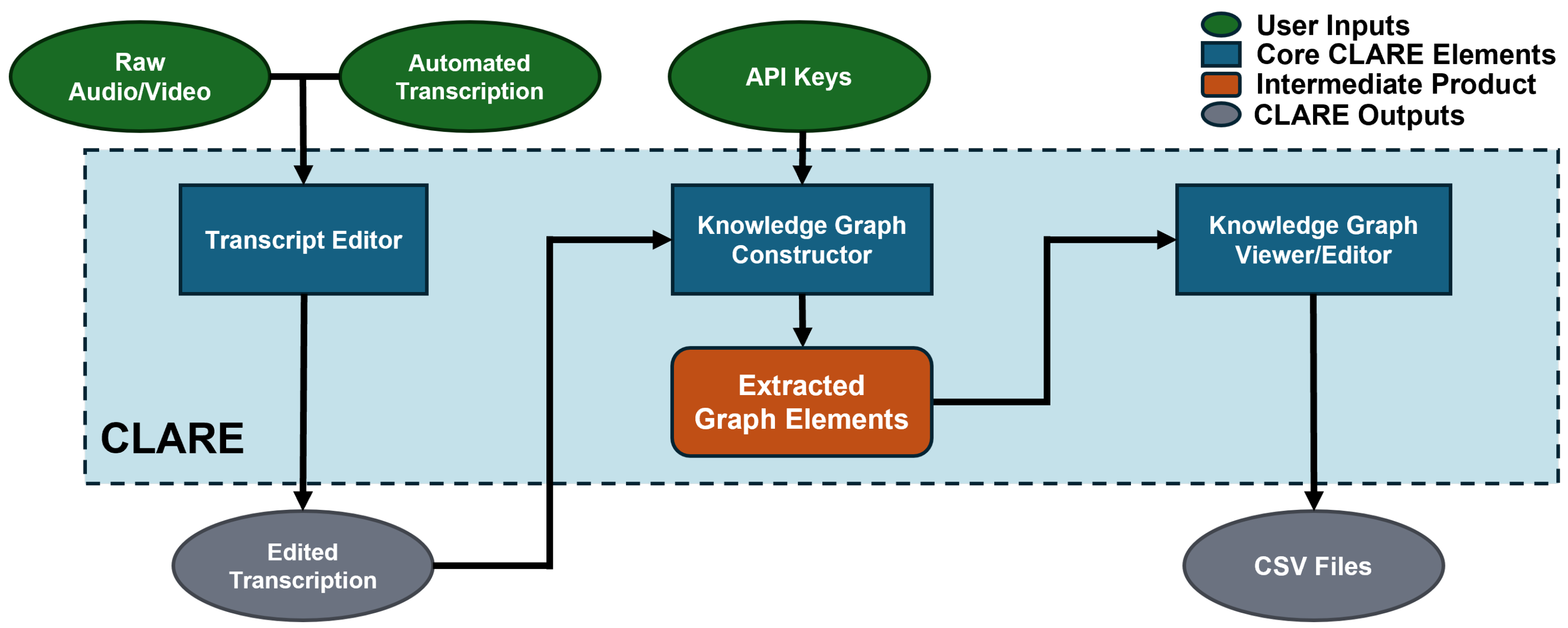
CLARE introduces a unified system for transcript-based KG construction composed of three modular, interoperable components. These are time-synchronized transcript correction, customizable KG construction, and interactive graph editing. Our primary contribution lies in extending AutoKG with a context-aware pipeline that transforms corrected transcripts into semantically labeled triples. We therefore begin by describing the KG construction process in detail. Afterward, we discuss the supporting components for transcript correction and graph refinement, which together enable seamless workflows for domain experts.

2.1. Knowledge Graph Construction

Our system’s KG construction uses a context-aware pipeline that extracts triples with awareness of surrounding discourse, which improves relation accuracy and coherence. In the “Knowledge Graph” tab, users can generate and visualize graphs from their transcripts within an integrated workspace that combines all generation, customization, and exploration tools. To accommodate diverse research needs, we provide model flexibility through the LiteLLM Python package, which supports independent selection of embedding models and LLMs from a variety of providers. These options include both cloud-based services and local execution through Ollama. With LiteLLM, users may run Ollama models on a local server for either embeddings or LLMs, gaining the privacy and cost benefits of on-device inference. In addition, bundled sentence-transformers models are available for local embeddings, which are lightweight enough to run directly within the application. These local choices reduce costs and improve speed while keeping sensitive data off external servers.

CLARE permits many model choices through LiteLLM and sentence-transformers. For the experiments reported in this paper, we used OpenAI’s gpt-4o-mini for all LLM prompting tasks (entity extraction, entity consolidation, and relation extraction) and sentence-transformers’ all-mpnet-base-v2 for text and entity embeddings. Relation extraction evaluated up to 30 candidate pairs per request and the dynamic threshold was set to 50%. The LLM prompts and specific configurations used for our evaluation are available in the Supplementary Materials and our Github page at https://github.com/ryanwaynehenry/CLARE (accessed on 26 September 2025), along with the full source code and executable for CLARE.

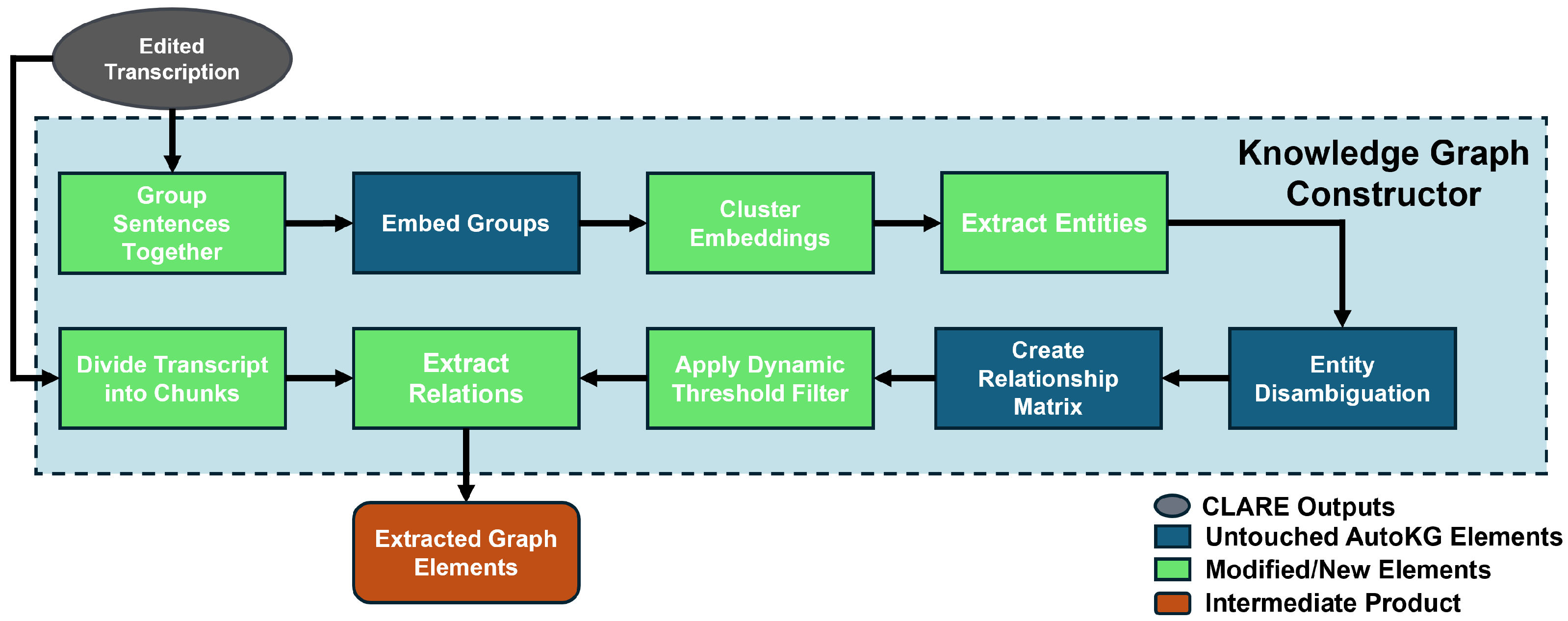
The knowledge graph construction process is initiated by the user within the interface. Before generating a graph, users may provide a central theme to filter irrelevant entities and may also set advanced parameters through the clustering options dialog box. Once ready, they can click the generate KG button to begin graph creation. Our system, illustrated in Figure 3, extends the AutoKG framework [23] by adding semantic relations between nodes and introducing modifications that improve context sensitivity and control over clustering behavior.

The KG process begins by preprocessing the input transcript through block-level segmentation and embedding to transform raw text into a form suitable for clustering. Adjacent transcription cells from the same speaker are concatenated to form discourse blocks. Let the sequence of raw utterances be denoted as $\{u_1,u_2,\dots ,u_n\}$. The segmentation function S produces a sequence of segments $\{s_1,s_2,\dots ,s_m\}$, where each $s_i$ satisfies the constraint $|s_i|\le 100$ words and aligns with sentence boundaries. Each segment $s_i$ is then passed through an embedding function $f:\mathcal{T}\to {\mathbb{R}}^d$, where $\mathcal{T}$ is the space of text segments and d is the embedding dimension. This yields a set of vectors $X=\{x_1,x_2,\dots ,x_m\}$ with $x_i=f\left(s_i\right)$. These vectors are used to capture the semantic content of the transcript in a high-dimensional space.

To identify thematically similar segments, the system applies the k-means clustering algorithm to the embedded set X. Users may specify the number of clusters k and the maximum number of entities per cluster l in the advanced options. If l is not provided, a preset default is used. If k is not provided, the system determines it automatically by evaluating several candidate values of k and selecting the one that maximizes the average silhouette coefficient $\overline{s}$. The silhouette coefficient measures clustering quality by comparing the cohesion of a point within its own cluster against its separation from other clusters. It is defined as

$$\overline{s}={\displaystyle \frac{1}{m}}\sum _{i=1}^m{\displaystyle \frac{b\left(i\right)-a\left(i\right)}{max\left\{a\right(i),b(i\left)\right\}}}$$

where $a\left(i\right)$ is the average intra-cluster distance for point $x_i$ and $b\left(i\right)$ is the lowest average inter-cluster distance to any other cluster. A higher value of $\overline{s}$ indicates better-separated and more cohesive clusters [29]. The clustering procedure yields a set of k clusters, either user-defined or chosen by silhouette-based selection, that are then processed independently.

After clustering the block embeddings, the system extracts entities (keywords) from each cluster using the AutoKG procedure [23]. Let cluster $C_j$ contain segments $\{s_{j1},\dots ,s_{j{n}_j}\}$ with embeddings $\{x_{j1},\dots ,x_{j{n}_j}\}$. From $C_j$, we sample $2c$ segments, with c nearest to the cluster centroid and c chosen at random, and prompt the LLM to propose up to l candidate entities. This produces the candidate set $K_j$ with $\left|K_j\right|\le l$. The system maintains a global entity set $\widehat{\mathcal{E}}$, which has each candidate’s set $K_j$ added to it. Once all the clusters have had their candidates extracted, the LLM is given $\widehat{\mathcal{E}}$ to consolidate duplicates, split overly broad items, and remove low-utility items from the concatenated list of candidates. The resulting $\mathcal{E}$ serves as the node vocabulary for downstream association.

For each entity $e_i\in \mathcal{E}$, we compute its embedding $y_i=f\left(e_i\right)$. We use this embedding to identify which texts are most and least similar in semantic meaning to a given entity based on cosine similarity.

$$d_{\angle }(y_i,x_j)=arccos\left({\displaystyle \frac{y_i^{\top }{x}_j}{\parallel y_i\parallel \parallel x_j\parallel }}\right)$$

Like in AutoKG, we apply Graph Laplacian Learning on X to obtain association scores between an entity and each text [23]. In Graph Laplacian Learning, we first select seed nodes by labeling the $n_1$ closest blocks to $y_i$ as positive (score 1) to indicate a strong relationship and the $n_2$ farthest blocks as negative (score 0) to indicate no relation. It then assigns scores to all remaining text blocks, requiring each score to equal the weighted average of its neighbors’ values. This iterative process propagates the seed labels through the graph until a stable equilibrium is reached [30]. Let h be the function produced by Graph Laplacian Learning, yielding a function $h(y_i,x_j)\in [0,1]$ that measures the association between entity embedding $y_i$ and block embedding $x_j$. To convert these continuous scores into binary associations, we define the indicator function $\eta (y_i,x_j)$ as

$$\eta (y_i,x_j)=\left\{\begin{array}{cc}1\hfill & \mathrm{if}h(y_i,x_j)\ge 0.5,\hfill \\ 0\hfill & \mathrm{if}h(y_i,x_j)<0.5.\hfill \end{array}\right.$$

where we set the threshold of $0.5$, so that only texts with high values of correlation will be associated with entity. We then form the set $A_{y_i}$ that encompasses all block embeddings from X that are linked to entity $y_i$.

$$A_{y_i}=\{x_j\in X\mid \eta (y_i,x_j)=1\}.$$

Using these sets, we create an entity–entity adjacency matrix $W\in {\mathbb{R}}^{M\times M}$, where $M=\left|\mathcal{E}\right|$

$$W_{ij}=|A_{y_i}\cap A_{y_j}|,$$

which counts how many blocks are jointly associated with $y_i$ and $y_j$. This yields symmetric, nonnegative integer weights between entities that indicate how strongly connected the two are likely to be. We remove self-edges by setting the diagonal to zero, $W_{ii}=0$.

We will use this matrix to identify which entities are likely to have relationships between them. The entities will form the nodes of the KG and the relationships will be the edges that connect them. The user has the ability to set a dynamic threshold based on a selected percentile of the edges they would like to evaluate. Let $p\in [0,100]$ be the user-selected retention percentile. The pipeline chooses a threshold h so that p% of the nonzero off-diagonal entries of W are at least h. We then overwrite W in place by setting

$$W_{ij}\leftarrow \left\{\begin{array}{cc}{W}_{ij}\hfill & \mathrm{if}i\ne j\mathrm{and}{W}_{ij}\ge h,\hfill \\ 0\hfill & \mathrm{otherwise}.\hfill \end{array}\right.$$

This keeps roughly the top $p\%$ of nonzero edges and zeros the rest, preventing those relationships from being considered. This pruning step is specific to our system and differs from AutoKG, which uses W without pruning. We then form the candidate pair set for relation extraction

$$\mathcal{P}=\{(e_i,e_j)\mid i<j,W_{ij}>0\}.$$

Rather than relying solely on the unidirectional weight $W_{ij}$ to represent relationships between entities as in AutoKG [23], the pipeline generates a short relation phrase by using the source text as context. The pipeline begins by querying an LLM to determine whether a meaningful relationship exists between entity pairs and to identify its form. First, the full transcript T is divided into overlapping chunks $\left\{T_k\right\}$ of at most $\lambda =t-m_{\mathrm{safe}}$ tokens, where t denotes the model’s token limit and $m_{\mathrm{safe}}$ is a safety margin that ensures there are enough tokens for the prompt and entity pairs. These chunks are generated by the sliding-window procedure in Algorithm 1, which enforces an overlap ratio o between the chunks. Within each chunk $T_k$, we extract the local candidate set

$${\mathcal{P}}_k=\left\{(e_i,e_j)\in \mathcal{P}\mid e_i,e_j\mathrm{appear}\mathrm{in}{T}_k\right\}$$

which contains all entity pairs co-occurring in that chunk. To balance efficiency and accuracy, we prompt the LLM to evaluate multiple potential relationships per query, partitioning ${\mathcal{P}}_k$ into batches of at most $B_{max}=30$ pairs. Each batch is sent to the user-selected LLM via LiteLLM with few-shot prompting [31]. The LLM responds with a list of $(e_i,r_{ij},e_j)$, where r is the semantic relation identified by the model. The response also includes the direction of the relation and a brief explanation for each relationship, as we found that having the LLM explain its reasoning improves the result. The LLM may also indicate that no relationship exists or that multiple relationships are present between each pair of entities. In the latter case, each relationship for a pair is listed together with its corresponding direction and explanation.

In some cases, an entity pair $(e_i,e_j)$ may never appear together within any transcript chunk, leaving the system without direct co-occurrence evidence to evaluate their relationship. This absence raises the question of how to gather sufficient context for such pairs. Users may enable a fallback option for these entity pairs in the advanced options menu. We define this set of entity pairs with

$${\mathcal{P}}_{\mathrm{miss}}=\{(e_i,e_j)\in C\mid \forall k,(e_i,e_j)\notin {\mathcal{P}}_k\}.$$

where ${\mathcal{P}}_{miss}$ represents the set of all entity pairs that never co-occur in the same transcript chunk.

When the fallback option is enabled, the system compiles, for each entity, a list of the sentence indices in which it appears within the transcript. Let the transcript be divided into sentences $\mathrm{\Sigma }=\{{\sigma }_1,\dots ,{\sigma }_q\}$. For an entity e, define the index set of mentions

$$\iota \left(e\right)=\{r\in \{1,\dots ,q\}\mid e\mathrm{appears}\mathrm{in}{\sigma }_r\}.$$

To provide local context, the set of sentences associated with an entity is expanded by adding the immediately preceding and following sentences for each of its members. This helps resolve pronouns and nearby references. We define the one-step neighborhood

$${\mathcal{B}}_1\left(r\right)=\{r-1,r,r+1\}\cap \{1,\dots ,q\},$$

and the contextual set for e

$$I\left(e\right)=\bigcup _{r\in \iota \left(e\right)}{\mathcal{B}}_1\left(r\right).$$

For a pair $(e_i,e_j)$, we take the combined context $I(e_i,e_j)=I\left(e_i\right)\cup I\left(e_j\right)$.

Algorithm 1 Sliding Window Transcript Chunking

1: Input T full transcript; t token limit; m safety margin; o overlap ratio $(0<o<1)$; $\mathrm{Tok}(·)$ token counter 2: Output ${\left\{T_k\right\}}_{k=1}^K$ chunks 3: $\lambda \leftarrow t-m_{\mathrm{safe}}$                                                                                ▹ max tokens per chunk 4: $\mathcal{L}\leftarrow \mathrm{split}\_\mathrm{words}(T)$                                                                                          ▹ list of words 5: $N\leftarrow \left|\mathcal{L}\right|$ 6: Initialize empty list $\left\{T_k\right\}$ and empty buffer B 7: $N_s\leftarrow min(20,N)$                                                                                ▹ sample size in words 8: ${\tau }_s\leftarrow \mathrm{Tok}\left(\mathrm{join}\left(\mathcal{L}[1...N_s]\right)\right)$                                                                  ▹ tokens in the sample 9: $\rho \leftarrow {\displaystyle \frac{N_s}{{\tau }_s}}$                                                                                       ▹ words per token estimate 10: ${\delta }_{\mathrm{tok}}\leftarrow \lfloor \lambda ·o\rfloor$                                                                      ▹ overlap measured in tokens 11: ${\delta }_w\leftarrow \lfloor {\delta }_{\mathrm{tok}}·\rho \rfloor$                                                                     ▹ overlap measured in words 12: $i\leftarrow 1$ 13: while  $i\le N$  do 14:     $end\leftarrow min(i+{\delta }_w-1,N)$ 15:     $\mathit{cand}\leftarrow \mathrm{join}(B,\mathcal{L}[i...end\left]\right)$ 16:     if $\mathrm{Tok}\left(\mathit{cand}\right)<\lambda$ then 17:         $B\leftarrow \mathit{cand}$ 18:         $i\leftarrow end+1$ 19:     else 20:         binary search for maximal fit 21:         $low\leftarrow i,high\leftarrow end,best\leftarrow i,count\leftarrow 0$ 22:         while $low\le high$ and $count<6$ do 23:            $mid\leftarrow \lfloor (low+high)/2\rfloor$ 24:            $\mathit{test}\leftarrow \mathrm{join}(B,\mathcal{L}[i..mid\left]\right)$ 25:            if $\mathrm{Tok}\left(\mathit{test}\right)\le \lambda$ then 26:                $best\leftarrow mid,low\leftarrow mid+1$ 27:            else 28:                $high\leftarrow mid-1$ 29:            end if 30:            $count\leftarrow count+1$ 31:         end while 32:         finalize current chunk 33:         $B\leftarrow \mathrm{join}(B,\mathcal{L}[i...best\left]\right)$ 34:         append B to $\left\{T_k\right\}$ 35:         prepare overlap buffer 36:         $\omega \leftarrow \lfloor \lambda ·o·\rho \rfloor$                                                                                ▹ overlap size in words 37:         $B\leftarrow (w_{\nu -\omega +1},\dots ,w_{\nu }),B=(w_1,\dots ,w_{\nu })$                                ▹ retain last $\omega$ words in buffer 38:         $i\leftarrow best+1$ 39:     end if 40: end while 41: return  $\left\{T_k\right\}$

We then group pairs in ${\mathcal{P}}_{\mathrm{miss}}$ by a greedy procedure described in Algorithm 2. The goal is to reuse overlapping sentences and to keep the number of groups small. Each group g must satisfy two constraints. The group size satisfies $\left|g\right|\le B_{max}$, with $B_{max}=30$. The concatenated context of its sentences must fit within the model budget $t-m$ tokens. For each pair, the algorithm places it in the group that results in the minimal increase in token count, ensuring that all constraints remain satisfied. Once all the groups are finalized, sentences in each group are concatenated in transcript order. Ellipses are inserted between non-adjacent sentences to signal discontinuity to the model. If the context for a single pair exceeds the token budget, we truncate that context to fit while preserving the most relevant sentences. After all groups are formed, we send each group context $T_g$, together with its pair set ${\mathrm{\Pi }}_g$, to the selected LLM using few-shot prompting. The LLM responds with the same format of triples, direction, and explanation as it did for the co-occurring pairs.

Algorithm 2 Fallback Relationship Extraction for Non-Co-Occurring Pairs

1: Input non co–occurring pairs ${\mathcal{P}}_{\mathrm{miss}}$; transcript T; token limit t; safety margin m; max batch size $B_{max}$; token counter $\mathrm{Tok}(·)$; mention-indexing function $\iota \left(e\right)$; extraction procedure $\mathsf{RelExtract}(\mathrm{context},\mathrm{pairs})$ 2: Output triples for pairs in ${\mathcal{P}}_{\mathrm{miss}}$ 3: $\lambda \leftarrow t-m_{\mathrm{safe}}$                                                                        ▹ token budget per query 4: if $\mathrm{Tok}\left(T\right)\le \lambda$ then          ▹ if the full transcript fits, use it once for all pending pairs 5:     $\mathsf{RelExtract}(T,{\mathcal{P}}_{\mathrm{miss}})$ 6:     return 7: end if 8: Split T into sentences $\mathrm{\Sigma }=({\sigma }_1,\dots ,{\sigma }_q)$                               ▹ sentence segmentation 9: for  $k=1$  to  q  do 10:     ${\tau }_k\leftarrow \mathrm{Tok}\left({\sigma }_k\right)$                                                              ▹ token count per sentence 11: end for 12: Initialize empty list $\mathcal{L}$                                                 ▹ will hold tuples $(p,J_p,c_p)$ 13: for all  $p=(e_i,e_j)\in {\mathcal{P}}_{\mathrm{miss}}$  do 14:     ${\iota }_i\leftarrow \iota \left(e_i\right),{\iota }_j\leftarrow \iota \left(e_j\right)$                               ▹ indices where each entity appears 15:     $J_p\leftarrow \left({\bigcup }_{r\in {\iota }_i}{\mathcal{B}}_1\left(r\right)\right)\cup \left({\bigcup }_{r\in {\iota }_j}{\mathcal{B}}_1\left(r\right)\right)$          ▹ context indices using a one–step neighborhood 16:     $c_p\leftarrow {\sum }_{k\in J_p}{\tau }_k$                                                  ▹ token cost of the pair’s context 17:     if $c_p>\lambda$ then              ▹ trim if a single pair’s context exceeds the budget 18:         Select a subset $J_p^{\prime }\subseteq J_p$ emphasizing indices near ${\iota }_i\cup {\iota }_j$ such that ${\sum }_{k\in J_p^{\prime }}{\tau }_k\le \lambda$ 19:         $J_p\leftarrow J_p^{\prime }$,    $c_p\leftarrow {\sum }_{r\in J_p}{\tau }_r$ 20:     end if 21:     Append $(p,J_p,c_p)$ to $\mathcal{L}$                  ▹ record pair, its context indices, and cost 22: end for 23: Sort $\mathcal{L}$ by $c_p$ in descending order         ▹ pack larger contexts first to maximize reuse 24: Initialize empty group list $\mathcal{G}$ 25: for all  $(p,J_p,c_p)\in \mathcal{L}$  do 26:     Find $g\in \mathcal{G}$ minimizing the marginal token increase 27:     $\mathrm{\Delta }(g,p)={\sum }_{k\in J_p\setminus J_g}{\tau }_k$        ▹ measures the extra token cost of adding p to g 28:     ${\mathrm{\Pi }}_g$,    $J_g$             ▹ the set of entity pairs in g, the set of sentence indices in g. 29:     Adding $(p,J_p,c_p)$ to a group is subject to two constraints 30:        1. $|{\mathrm{\Pi }}_g|<B_{max}$ 31:        2. ${\displaystyle \sum _{k\in J_g\cup J_p}{\tau }_k\le \lambda }$ 32:     if such a group g exists then                  ▹ greedy packing with overlap reuse 33:         ${\mathrm{\Pi }}_g\leftarrow {\mathrm{\Pi }}_g\cup \left\{p\right\}$,    $J_g\leftarrow J_g\cup J_p$,    $c_g\leftarrow {\sum }_{r\in J_g}{\tau }_r$ 34:     else 35:         Create a new group g with ${\mathrm{\Pi }}_g\leftarrow \left\{p\right\}$, $J_g\leftarrow J_p$, and $c_g\leftarrow {\sum }_{r\in J_g}{\tau }_r$; append to $\mathcal{G}$ 36:     end if 37: end for 38: for all $g\in \mathcal{G}$ do                   ▹ build context strings and extract relations 39:     Let ${\mathrm{\Sigma }}_g$ be the sentences indexed by $J_g$, ordered increasingly by index. 40:     Build $T_g$ by concatenating ${\left\{{\sigma }_k\right\}}_{k\in {\mathrm{\Sigma }}_g}$, inserting “...” between nonadjacent indices 41:     $\mathsf{RelExtract}(T_g,{\mathrm{\Pi }}_g)$ 42: end for

For final processing, we merge the outputs across all the groups, for both co-occurring and fallback pairs. For each candidate triple $(e_i,r,e_j)$ returned by the model with direction tag $d\in \{\mathrm{forward},\mathrm{reverse},\mathrm{none}\}$, we proceed as follows. If $d=\mathrm{forward}$, we keep $(e_i,r,e_j)$. If $d=\mathrm{reverse}$, we swap the arguments and form $(e_j,r,e_i)$. If $d=\mathrm{none}$, we discard the item. The finalized set of directed triples defines the edges of the KG, denoted by $\mathrm{\Gamma }$, where each node corresponds to an extracted keyword. We pass $\mathrm{\Gamma }$ to the visualizer for interactive exploration and filtering.

2.2. Interface Design and Functionality

This section describes the two workspaces that support end-to-end analysis in our system. The “Transcript Editor” enables precise, time-aligned correction of source material. The “Knowledge Graph” serves as a workspace for graph generation, visualization, and post hoc editing. Together, they allow a workflow that begins with raw media and ends with an editable, exportable KG without external conversion utilities.

2.2.1. Transcript Editor

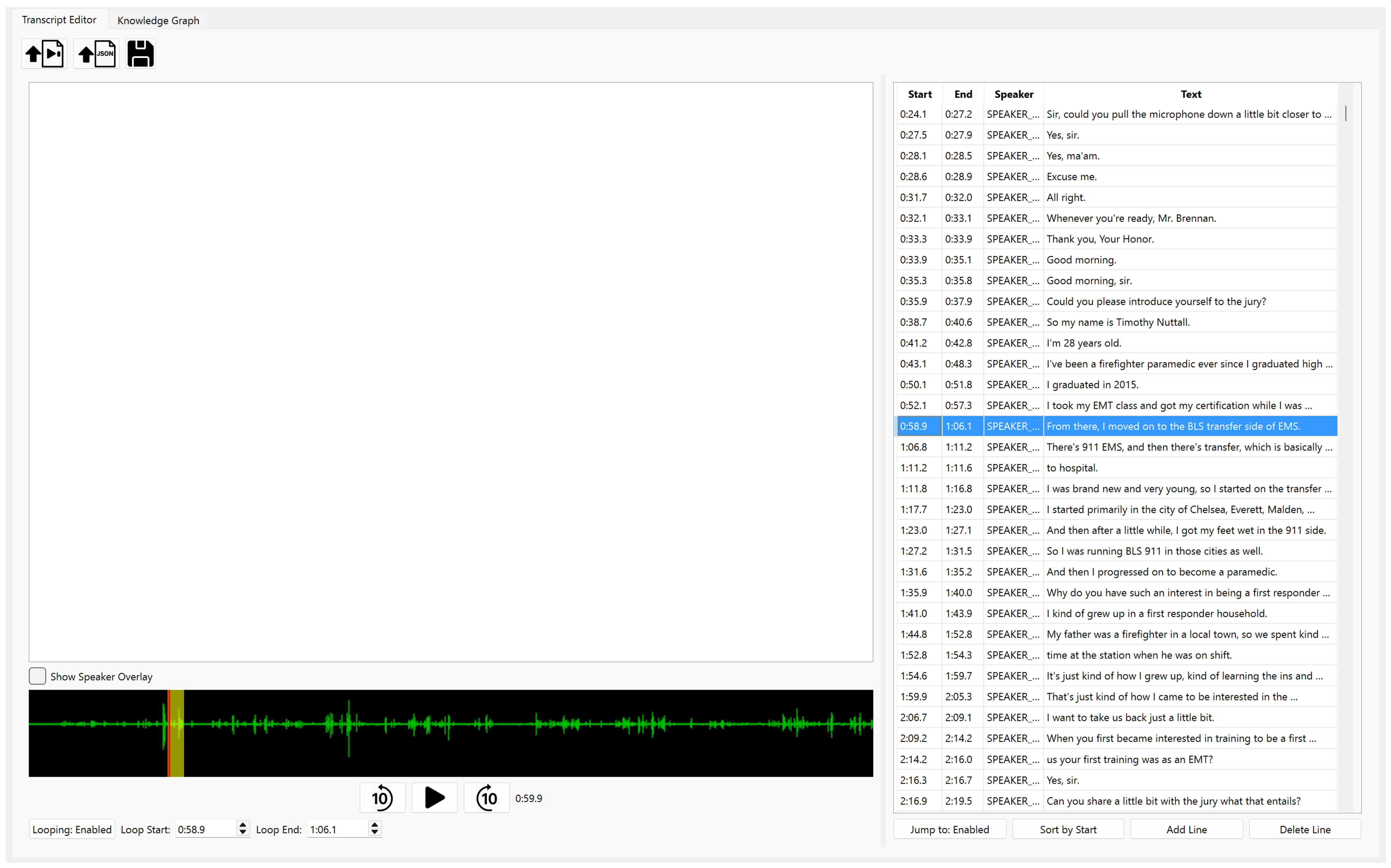
The transcript editor shown in Figure 4 presents the source media and its time-aligned transcript side by side so that users can verify and correct content with minimal effort. Two JavaScript Object Notation (JSON) formats are supported for import. The first is a simple per-line structure with start time, end time, speaker label, and text. The second is the JSON file produced by the aTrain GUI [8]. By supporting aTrain’s output, the editor lets users move from source media to an edited transcript and KG using only two applications. No intermediate conversion utilities are required. This lowers the technical barrier for domain experts outside computer science and aligns with our goal of reducing reliance on programmer workflows.

The design supports efficient transcription by placing playback tools and transcript editing in dedicated panels. The left panel contains a waveform visualization with standard playback controls and a timeline slider, allowing users to navigate recordings efficiently. If the media is a video, it is displayed in this panel above the waveform to keep the playback and visual context together. A vertical bar indicates the current playback time, giving users a clear reference point for precise positioning within the audio. When a transcript segment is selected in the right panel, the corresponding region of the waveform is automatically highlighted between its start and end times. The right panel contains an editable table of transcript rows with columns for start time, end time, speaker label, and text. By default, selecting a transcript row moves playback to the beginning of that segment, and it will automatically repeat the audio between its start and end times. This looping is especially helpful when passages are unclear or when speakers overlap. Simple toggles control both the seek and looping features, so users who prefer full manual navigation can turn them off at any time.

Editing operations are designed to be immediate and intuitive, allowing users to make corrections directly within the transcript without additional steps. Rows can be inserted, moved, or deleted. Edits are applied directly in place within the same interface, allowing users to adjust timing, text, or speaker labels without breaking their workflow. When users modify start or end times, the highlighted region of the waveform updates instantly to reflect the change, providing immediate visual feedback. When transcript rows are reordered or start and end times are adjusted, the transcript can drift out of chronological sequence. Users can restore the chronological sequence of the transcript by clicking the “Sort by Start Time” button below it. This ability to quickly recover a coherent timeline is particularly useful during heavy editing, where structural changes might otherwise leave the transcript fragmented or confusing. Users have the option to save the transcript at any stage, either for resuming editing later or for archiving as the finalized version.

The editor is integrated with the KG workflow so that graphs are generated directly from the transcript. In the intended CLARE process, the first steps are to refine the transcript thoroughly and then build the graph. If later exploration reveals a mistake such as a spurious node, a missing entity, or an ambiguous relation, the user can return to the editor, correct the transcript, and regenerate. When the issue is small, the user may instead apply a targeted fix in the graph view, which can be faster than a full rebuild for long transcripts. After each build, search and filtering in the graph view help verify the effect of changes. This process balances up-front transcript quality with selective corrections and produces a transcript that is accurate for archival use and well structured for entity extraction.

Transcript fidelity directly affects the reliability of the KG. Precise segment boundaries align entity mentions with the correct text blocks, which stabilizes association scores and reduces spurious co-occurrences. Consistent speaker labels reduce the likelihood of false merges during clustering, ensuring that utterances from different individuals remain properly separated. Clean punctuation and sentence boundaries improve segmentation and embeddings. The editor is not only a convenience. It serves as a control surface for improving downstream graph construction through small, targeted corrections that can be verified in the visualization.

2.2.2. Knowledge Graph Visualizer and Editor

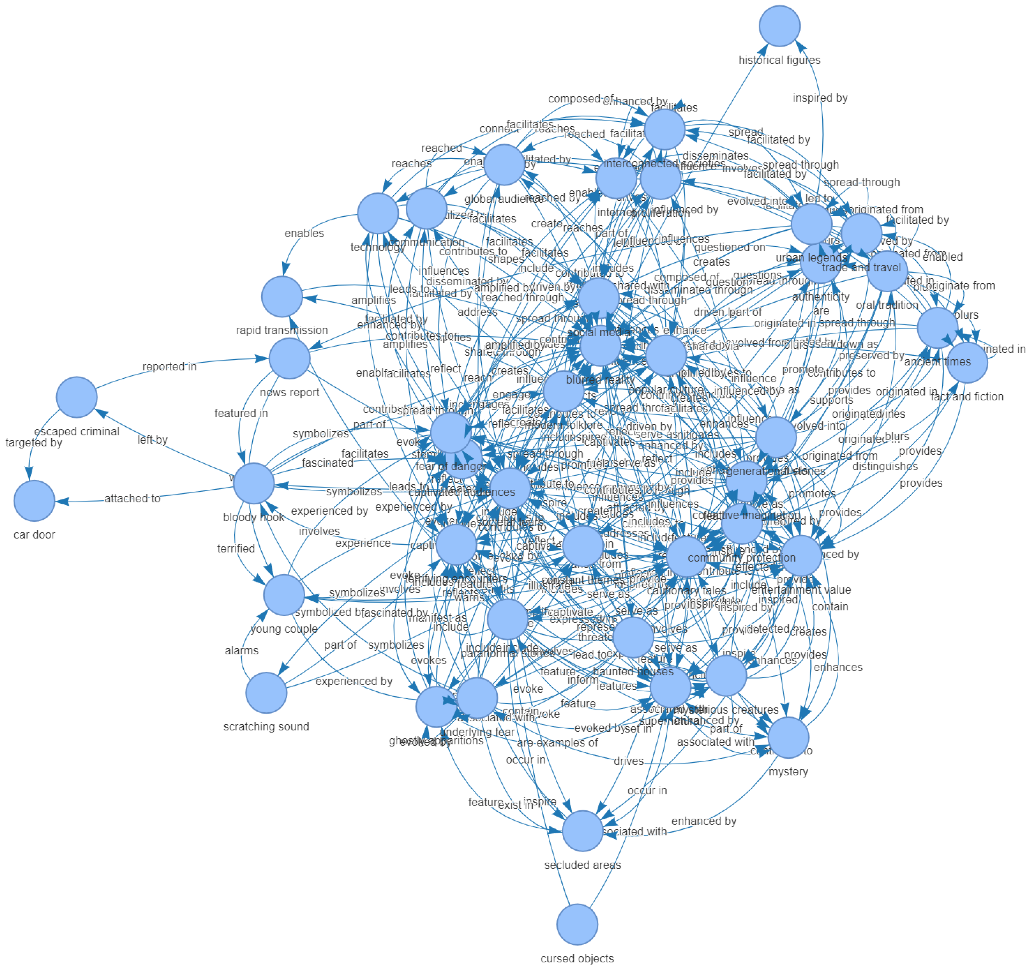
The Knowledge Graph tab shown in Figure 1 includes a ribbon at the top of the window that groups KG generation controls, input and output options, and later editing tools. The KG generation controls section includes a Central Topic field that accepts a phrase that filters off-topic entities and edges. The adjacent Clustering Options button opens an advanced dialog for clustering and relation-extraction parameters. Users can set the number of clusters for grouping text segments and the per-cluster cap on candidate entities. Raising this cap increases the number of entities considered and typically produces a larger graph at the cost of a longer processing time. The dialog also includes a Dynamic Threshold setting that keeps only the top $p\%$ of candidate edges by score. Next to the Clustering Options button in the ribbon are the Model Selection menus. Users must choose an embedding model and a language model, then provide credentials through the API Keys button, which stores keys locally. Both the API keys used by Hosted services and the server address required for local deployments will be provided by the user in the API Keys window. After the model selections keys are provided, and any optional parameters are set, the user clicks the Generate KG button to run the pipeline on the currently loaded transcript.

The Knowledge Graph view complements automated construction with an interactive workspace for exploration and refinement. Graphs can be generated directly from the transcript pipeline or imported from CSV files that contain node and edge lists. A search bar in the upper-right corner lets users locate entities by name. To manage visual complexity, two filters provide focused views. The Direct Connections filter shows each selected entity together with its immediate neighbors and hides unrelated edges. The Overlapping Connections filter uses a stricter rule, displaying only relationships between entities within the current selection. This focused visibility enables users to examine interaction patterns in densely connected regions without being distracted by superfluous information.

At the core of the interface is the canvas, which displays the graph and allows users to manipulate it directly. Users can drag entities to improve legibility, uncover crossings, or group related concepts. Common editing actions are placed prominently in the top ribbon, allowing users to delete relationships, remove nodes, or reverse edge directions with minimal effort. The ribbon layout and single-click controls make these corrections efficient, so that graph adjustments remain a seamless part of the analytical process. A collapsible side panel exposes the advanced editing options. Researchers can add new nodes, rename existing nodes, merge duplicates into a single entity, and create or adjust relationships. The interface includes a selection buttons that speed up filtering and advanced edits. Instead of typing names manually, users can click directly on nodes or relationships to add them to the active filter or editing panel.

KG construction is a complex task in which some errors are to be expected. Our interface addresses this reality by emphasizing efficient error detection and correction, enabling users to iteratively refine the graph instead of relying on a one-time, error-free output. Users explore the automatically generated structure with search and filters, then apply editing operations to refine it, including by removing spurious nodes, correcting edge directions, merging entities, and adding missing links. Small issues in the generated KG should be corrected using this interface. But for severe, cascading issues, the root cause is likely an error in the transcript itself, and it is likely more efficient to correct the issue there and regenerate the KG. This loop supports steady convergence toward a representation that matches the user’s understanding of the source material.

When a graph meets the user’s needs, it can be exported as CSV files for nodes and edges. Exported CSV files can be reloaded into CLARE at any time for continued editing and exploration, or imported into external environments such as Neo4j for extended analysis. Together, the transcript editor and graph viewer form a unified workflow; one ensures accurate input, and the other provides the means to refine and interpret its output. This integration allows users to iteratively improve both transcript quality and graph clarity within a single environment.

3. Results

We carried out our experiments on the MINE benchmark, which provides 105 Wikipedia-style articles drawn from a wide range of topics (e.g., butterfly life cycles, urban legends, ancient cultures, AI ethics, and cooking). Each article is paired with fifteen ground-truth facts. For every fact, MINE generates a context from the KG. This process begins by loading the graph’s nodes and edges, then embedding both the fact and the node labels into the same vector space. For each fact, cosine similarity is used to compare the fact’s embedding with each node embedding, and the k most similar nodes are selected as entry points. Once the seed nodes are identified, MINE constructs the context by forming a set of all triples in which each of these nodes participates. To capture the broader structure, it then expands outward. For each of the selected nodes, it follows their neighbors in the graph up to a depth of two, adding the associated triples at each step. The union of these triples is concatenated into a single textual context. This context, along with the ground-truth fact, is provided as input to an LLM, which is prompted to judge whether the fact is supported by the evidence in the context. The model returns a binary judgment for each fact. We define fact accuracy as the percentage of the fifteen facts that are marked as supported for each article.

We began by tuning CLARE hyperparameters on the first five MINE articles. Increasing the entity cap per cluster improved node coverage, but also introduced many low-value edges. To control for this, we use the dynamic threshold to filter out weaker similarity scores. This pruning cut processing time for the pilot set nearly in half, with only a negligible effect on fact accuracy. The resulting KGs were large and densely connected. Figure 5 shows an example graph from an article on urban legends, where numerous relationships link entities both within and across clusters.

The final configuration adopted for the MINE evaluation was a cap of thirty entities per cluster and the dynamic threshold set to 50%. We used GPT-4o-mini for relation extraction to balance accuracy, runtime, and cost. During early testing, we also evaluated GPT-4o and found that it produced slightly better results, but GPT-4o-mini’s performance was satisfactory while being substantially cheaper and faster. For embeddings, we tested both OpenAI’s text-embedding-3-large and the Sentence-Transformers model all-mpnet-base-v2. Since performance differences were negligible, we adopted all-mpnet-base-v2 because it is faster, cheaper, and can be run locally. Our choice of GPT-4o-mini and all-mpnet-base-v2 was also motivated by accessibility; we sought to demonstrate that CLARE performs well even with modest models that smaller research groups are more likely to adopt.

We evaluated CLARE on all 105 MINE articles. On the full set, CLARE achieved a mean fact accuracy of 83.3% with a standard deviation of 13.05%. For direct, like-for-like comparisons with prior systems, we restrict reporting to the 87 articles for which KGGen, GraphRAG, OpenIE, and CLARE all have results. On this overlapping set, CLARE’s mean fact accuracy was 82.1% with a standard deviation of 12.96%. Figure 6 shows that most article-level accuracies on this set fall between 73.3% (11/15 facts correct) and 100%, with a kernel density estimate (KDE) peak just over 90%. A small number of articles fall below 67%, largely due to relevant entities not being extracted from the text.

The non-CLARE curves in Figure 6 are derived from raw evaluation files released by the KGGen authors on GitHub [32], which also include baselines for OpenIE and GraphRAG [4,22]. Because those releases omit a few articles for each baseline, all cross-system statistics are computed on the 87-article intersection.

Table 2. Distribution of article-level fact accuracy scores in the MINE benchmark, reported as the number of articles at each accuracy level.

Percent of Facts in KG	GraphRAG	OpenIE	KGGen	CLARE
0.0%	1	4	2	0
6.7%	0	7	0	0
13.3%	2	7	1	0
20.0%	4	12	0	0
26.7%	4	20	2	0
33.3%	13	14	2	0
40.0%	11	8	4	1
46.7%	12	4	7	0
53.3%	9	5	11	3
60.0%	12	3	8	4
66.7%	8	2	10	9
73.3%	10	1	11	8
80.0%	0	0	13	16
86.7%	0	0	10	15
93.3%	1	0	4	24
100.0%	0	0	2	7

presents the raw values corresponding to the histogram, and the mean fact accuracy for each model appears in

Table 3. Mean fact accuracy of different systems on the MINE benchmark.

System	Mean Fact Accuracy
OpenIE	29.2%
GraphRAG	48.3%
KGGen	64.8%
CLARE (Ours)	82.1%

. On the overlap, CLARE achieved 82.1% fact accuracy, exceeding KGGen, GraphRAG, and OpenIE by 17.9%, 35.5%, and 52.9%, respectively. The primary trade-off for this improvement is runtime, as generating each article-level KG required roughly twenty-five minutes on our hardware, driven largely by the number of LLM calls.

To assess the robustness of these improvements, we applied Wilcoxon signed-rank tests [33] at the per-article level. The Wilcoxon tests use the pairwise article overlap between CLARE and each individual baseline, whereas the mean-accuracy comparison from Table 3 relies on the four-model intersection. Each baseline includes some article results that the other models do not have. As a result, both the mean differences $\mathrm{\Delta }$ and the number of articles included in each test in

Table 4. Wilcoxon signed-rank comparison of per-article accuracies against CLARE on MINE. $\mathrm{\Delta }$ reports CLARE − System in percentage points; positive values favor CLARE. Here, n is the number of matched articles, p is the Wilcoxon p-value, Z is the large-sample normal approximation, $r=\left|Z\right|/\sqrt{N}$ is the effect size, and the 99% CI is a percentile bootstrap confidence interval for the mean $\mathrm{\Delta }$.

System	n	p-Value	Z	r	Mean $\mathrm{\Delta }$	99% CI (Mean $\mathrm{\Delta }$)
KGGen	100	$3.85\times {10}^{-10}$	$-6.266$	$0.646$	$+17.93\%$	$[+11.80\%,+24.27\%]$
GraphRAG	94	$2.32\times {10}^{-16}$	$-8.210$	$0.856$	$+35.04\%$	$[+29.01\%,+40.92\%]$
OpenIE	99	$8.05\times {10}^{-18}$	$-8.605$	$0.869$	$+53.40\%$	$[+48.22\%,+58.52\%]$

slightly differ from those in Table 3. Table 4 summarizes the Wilcoxon test results, reporting p-values and rank-biserial effect sizes ($r=\left|Z\right|/\sqrt{N}$). Across all comparisons, p-values are far below conventional thresholds, like 0.05 or 0.01, and effect sizes are large ($r>0.6$), indicating that CLARE’s advantage is both statistically reliable and practically meaningful. We also provide 99% bootstrap confidence intervals for the mean paired differences; these exclude zero in all cases, reinforcing the notion that the observed gains are consistent across articles rather than due to random variation.

To evaluate the GUI’s effectiveness in supporting users to view, filter, and refine automatically generated KGs, we conducted an additional experiment. We selected the twenty-five lowest-performing KGs produced by CLARE and allocated fifteen minutes to improve each one. During this process, we were shown the facts each graph had missed in the original MINE evaluation and were free to add new nodes and relations or revise existing ones. The only constraint was that any newly created triples had to incorporate at least one existing node from the graph. After refinement, we reevaluated the graphs using MINE and compared the results. As shown in Figure 7, even these short interventions produced considerable gains, with the average KG’s fact accuracy increasing by 22.67%.

4. Discussion

Results on MINE indicate that CLARE provides a consistent advantage over prior approaches. Its context-aware extraction and broader edge search yield denser, more informative graphs that capture cross-sentence relations more reliably than baseline pipelines. The magnitude and consistency of the gains across articles suggest that the improvements arise from the pipeline’s design rather than chance variation in specific samples. That said, these advantages carry computational costs.

Although the resulting graphs are informative, they come with trade-offs. On our hardware, each article required roughly twenty-five minutes to generate a KG, driven largely by the number of LLM calls. Pilot runs also showed that many low-value edges contribute little to downstream fact checking yet are expensive in aggregate. While the MINE benchmark demonstrates CLARE’s effectiveness on descriptive texts, our analysis indicates that a single undifferentiated graph is less suitable for domains where speakers advance conflicting claims or hold distinct roles, such as legal hearings, debates, or biomedical consultations. Addressing these cases will require explicit modeling of speaker roles and disagreements, which we identify as an important direction for future enhancement.

In the second evaluation, where we manually refined the twenty-five lowest fact accuracy KGs, we observed that substantial improvements could be achieved within a short time. During these corrections, we also gained insight into why many graphs failed to capture the missed facts. CLARE was effective at generating conceptual entities, but the graphs often omitted proper nouns, leaving out specific people, places, or objects mentioned in the text. Whether this limitation stems from the specific prompt, the choice of LLM, or the underlying methodology remains unclear and warrants further investigation. During the MINE evaluation, it was uncommon for graphs to include the correct entities but omit the relation linking them. This suggests that using the fiftieth percentile as the dynamic threshold did not substantially reduce KG quality, and that lowering the threshold further may still preserve strong performance.

5. Conclusions

CLARE was designed to close the tooling gap that separates domain experts from the benefits of automated KG technology. By combining a time-synchronized transcript editor, a model-agnostic graph generator, and an interactive visualizer in a single interface, the system allows users to move from an automated transcript to a structured, editable graph without writing code. When used in combination with tools like aTrain for initial transcription, CLARE supports an efficient end-to-end workflow from raw audio or video to a manually corrected KG derived from that recording. This workflow addresses the practical challenges identified in prior studies, including the steep learning curve of natural language processing pipelines, the high cost of external services, and the privacy restrictions that discourage cloud processing. Our results demonstrate that these barriers can be lowered with thoughtful interface design.

Overall, our results highlight two distinct insights. Firstly, a model-agnostic backend that supports both local embeddings and on-demand LLM calls gives users precise control over the privacy, performance, and cost trade-offs of their pipelines, and this design enabled CLARE to consistently outperform KGGen and GraphRAG in fact accuracy, supporting Hypothesis 1. Secondly, an integrated, analyst-focused interface makes KG construction accessible to domain experts without programming skills, and user refinements through this interface yielded measurable improvements in quality with modest effort, supporting Hypothesis 2.

A major enhancement planned for future work is stronger support for multi-speaker knowledge graphs. In many interviews, debates, or biomedical consultations, participants advance conflicting claims or play distinct roles, and a single undifferentiated graph can obscure these dynamics. To address this, we plan to assign speaker labels as properties on edges. In the interface, these labels will appear as differently colored edges with a legend indicating each speaker, and users will be able to filter the visualization to show or hide contributions from specific speakers. This capability will broaden CLARE’s applicability to domains such as legal transcripts, debates, and biomedical interviews, and it also lays the foundation for adapting CLARE to AI scribe scenarios, where structuring multi-speaker dialogue into a knowledge graph can assist physicians while preserving the fidelity of patient–clinician interactions.

Another direction for improvement is more consistent entity extraction, particularly for proper nouns such as specific people, places, and organizations. Our evaluation suggests that a major source of error stems from leveraging AutoKG’s entity extraction prompt, which asks the LLM to summarize blocks of text and extract keywords from them. This design tends to emphasize abstract entities such as ideas and events, while overlooking specific nouns that may appear only once in the text. To address this limitation, we plan to investigate enhanced extraction strategies, including tailored prompting techniques, hybrid methods that combine LLM outputs with traditional named entity recognition (NER), and post-processing steps designed to recover overlooked proper nouns. We also intend to explore normalization of the entity correlation matrix so that infrequently mentioned but strongly connected entities are retained rather than pruned. Together, these refinements will increase the completeness of the graphs and ensure more reliable coverage of factual content.

Finally, efficiency remains a practical concern. Each graph currently requires around twenty-five minutes to generate, driven largely by the number of LLM calls. To reduce this cost, we plan to explore strategies such as pruning low-confidence candidates more aggressively, caching embeddings for partial KG regeneration, and normalizing the entity correlation matrix to retain strong but infrequently mentioned entities. These refinements will make CLARE more scalable for larger collections of transcripts.