Enhanced Fault Detection in Bearings Using Machine Learning and Raw Accelerometer Data: A Case Study Using the Case Western Reserve University Dataset

Abstract

This study introduces a novel approach for fault classification in bearing components utilizing raw accelerometer data. By employing various neural network models, including deep learning architectures, we bypass the traditional preprocessing and feature-extraction stages, streamlining the classification process. Utilizing the Case Western Reserve University (CWRU) bearing dataset, our methodology demonstrates remarkable accuracy, particularly in deep learning networks such as the three variant convolutional neural networks (CNNs), achieving above 98% accuracy across various loading levels, establishing a new benchmark in fault-detection efficiency. Notably, data exploration through principal component analysis (PCA) and t-distributed stochastic neighbor embedding (t-SNE) provided valuable insights into feature relationships and patterns, aiding in effective fault detection. This research not only proves the efficacy of neural network classifiers in handling raw data but also opens avenues for more straightforward yet effective diagnostic methods in machinery health monitoring. These findings suggest significant potential for real-world applications, offering a faster yet reliable alternative to conventional fault-classification techniques.

1. Introduction

Rotating machines (RMs) represent a versatile class of mechanical equipment that finds extensive use across a wide range of industrial applications. These machines have earned a reputation for their robustness, low cost, and remarkable reliability, making them a vital component of numerous industrial processes [1]. RMs have the ability to convert electrical energy to mechanical energy and vice versa, thereby enabling a wide range of applications such as power generation, transportation, and manufacturing. Due to their versatility and importance, RMs have been the subject of significant research and development efforts to improve their performance, efficiency, and reliability [2].

As these machines are crucial for daily operations in various industries, there has been extensive research and development focused on understanding the types of faults that can occur, including their causes, early detection, and the condition monitoring of key components such as stators, rotors, shafts, and bearings. In fact, fault diagnosis and condition monitoring have been highly researched for almost two decades. Additionally, the Electric Power Research Institute (EPRI) conducted a survey in 2018 to determine the frequency of faults in the major components of induction motors (IMs), which are a primary type of RMs [1,3]. The survey findings revealed that a significant portion, specifically 41–42%, of IM failures are attributed to bearing defects, whereas 36% are related to stator defects. Given the paramount importance of bearings as the component most susceptible to faults in IMs/RMs, the central objective of this research paper is to offer a robust algorithm-based approach for accurately categorizing diverse bearing faults under varying load conditions. The objective is to provide valuable insights for major industries across the globe, including those in Pacific developing countries, with the aim of minimizing unscheduled downtime and reducing the associated expenses of repair and replacement.

The bearing comes in two sets, which are placed at both ends of the RM to support the rotating shaft and limit friction for free rotation. The inner and outer rings in the bearing are termed races, and in between the races are rolling elements called balls. However, the heavy reliance on rolling bearings in various operations, including harsh working environments and alternating loads, makes them the most susceptible component to faults [4,5]. Any form of physical damage on the inner or outer race or the ball’s surface is classified as a bearing fault, as illustrated in Figure 1 below. Additionally, it is worth noting that bearing faults can cause a range of issues, including increased vibrations, noise, and reduced efficiency, which can eventually lead to catastrophic failures if not addressed promptly. Therefore, it is crucial to regularly monitor bearings for the early detection of faults and timely maintenance to prevent any significant damage to the RM system.

Figure 1. Types of bearing faults and their locations [6].

Machine Learning Algorithms for Fault Identification and Diagnosis

The ultimate goal of fault diagnosis (FD) is to recognize the status of a targeted component, and then decisions are made based on whether maintenance is needed. The model-based approach and the data-driven approach are two existing methods of FD; the work of [7] states that the model-based approach requires abundant prior knowledge and poses difficulty in accurately establishing diagnosis models of composite components under complex conditions. On the other hand, data-driven models have been more attractive in developing various intelligent approaches. This method can effectively process machinery signals and accurately diagnose results with low requirements for prior expertise.

In the context of fault identification (FI), the research presented in [8] involves conducting a comparative investigation by utilizing two shallow machine learning (ML) models, namely support vector regression (SVR) and a relevance vector machine (RVM). The performance of these models in terms of probabilistic findings using random kernel functions for FI highlighted RVM performance as superior to that of the SVR algorithm. Liang-Yu [9] highlighted in this paper that treating feature selection and parameter optimization separately poses a restraint for SVRs and affects their prediction accuracy. Further, the author later referred to the above study and presented two bearing-fault schemes for FI and FD based on an RVM of vibration signals, i.e., two relevance models viewed as an observer and classifier. Another monitoring procedure highlighted in [10] involves using the stator current using motor current signature analysis (MCSA) and employing frequency spectral subtraction using various wavelet transforms to suppress dominant components. Discrete wavelet transform (DWT), wavelet packet decomposition (WPD), and stationary wavelet transform (SWT) are procedures for spectral subtraction [11,12].

While previous studies have utilized techniques such as preprocessing, dimensionality reduction, and feature selection to accurately classify bearing faults, limited research has been conducted on developing models to use raw data for this task. Therefore, the proposed research aims to address this gap by developing and using predeveloped models that can utilize raw accelerometer data to accurately predict the variance of faults in the motor’s bearing under changing loading levels. By avoiding intensive preprocessing and feature-extraction steps, the proposed model has the potential to reduce computational complexity and improve the accuracy of fault detection and identification. Furthermore, incorporating advanced machine learning techniques such as deep learning can further enhance the model’s performance. Overall, the proposed research aims to contribute to developing more accurate and efficient methods for fault detection and identification in rotating machinery.

The organization of the paper is as follows: Section 2 highlights the paper’s contributions; Section 3 provides an elaborate description of the CWRU bearing dataset; Section 4 provides insight into the proposed methodology; Section 5 graphically explores the raw data through scatter tools and appropriate dimensionality reduction techniques; Section 6 provides detailed information on all the classifier models to be used for the proposed methodology, along with the model hyperparameters; and Section 7 evaluates the results and provides justifications accordingly. The conclusion is presented in Section 8.

2. Paper Contribution

This paper presents a methodology for the fault classification of ball, inner-race, and outer-race faults at various loading levels using raw accelerometer signals. The vibration signals used in the study were obtained from the CWRU database. In the preprocessing step, the accelerometer signals were segmented into 500 window sizes with strides of 200 using the windowing method. Data exploration was conducted using PCA and t-SNE to visualize if the data were distinguishable. The paper evaluates the efficiency of neural network (NN)-based classifiers in classifying bearing-related faults without the assistance of any feature-extraction step. The proposed methodology combines NN-based classifiers, specifically multi-layer perceptron (MLPs), long short-term memory (LSTM), and convolutional neural networks (CNNs). The performance of the classifiers is evaluated based on four different metrics: specificity, precision, recall, and F1-score. The experimental results show that the proposed CNN variant classifiers achieve high accuracy rates in classifying the three bearing-related faults. Specifically, one-dimensional CNN, multiple kernel CNN, and two-dimensional CNN portray the best performance varying from approximately a 95% to a 99% accuracy rate, respectively, over the three loading levels.

The proposed methodology demonstrates a rational approach for accurate and efficient fault classification, contributing to advancing bearing-fault diagnosis. By accurately identifying the types of bearing faults, maintenance teams can schedule repairs or replacements before equipment failure occurs, reducing downtime and costs. This has practical implications for predictive maintenance in various industries, such as aerospace, automotive, and manufacturing. The study also contributes to the field of machine learning by demonstrating the effectiveness of using raw accelerometer signals for fault classification without the need for feature extraction. This approach can save time and computational resources, making it a promising direction for future research in other areas of fault diagnosis.

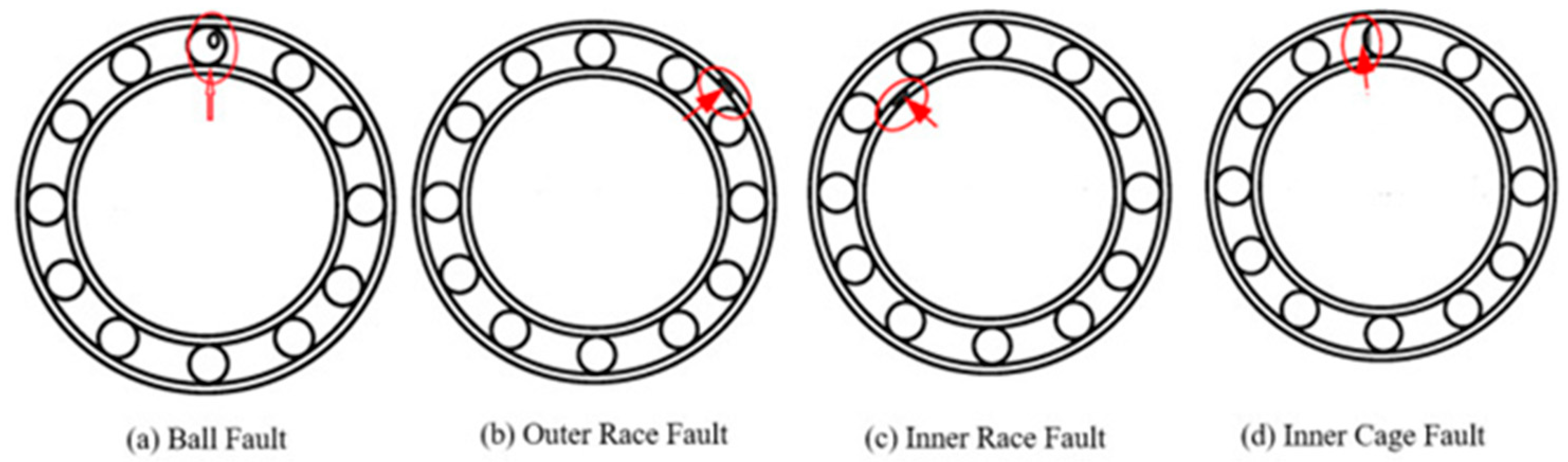
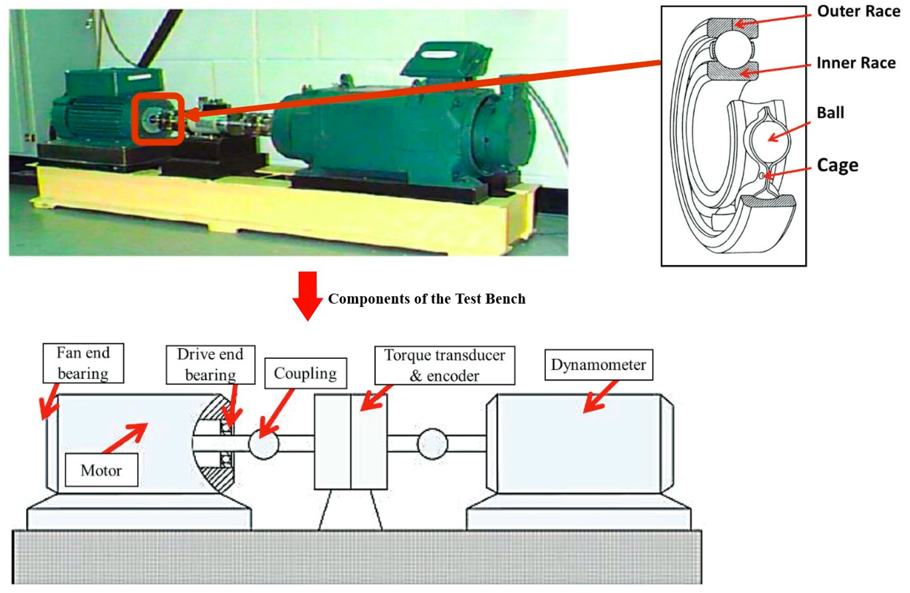
3. Data Description

The dataset from the CWRU [13,14] was used to evaluate the proposed methodology. Figure 2 shows the CWRU’s experimental rig for studying ball-bearing defects. Vibration measurements were acquired with three accelerometers placed in the 12 o’clock position on the housing of the drive end (DE) and fan end (FE). SKF deep-groove ball bearings of types 6205-2RS JEM and 6203-2RS JEM were employed for the DE end FE, respectively.

Figure 2. CWRU Motor Experimental Rig [14].

Electro-discharge machining generated different fault diameters ranging from 0.007 to 0.021 inches. Vibration signals were recorded at 48 kHz, under varying motor speeds from 1797 to 1720 rpm, and we used three motor-load operating conditions, denoted as no-load condition (L0): 0% of the nominal load; half-loaded condition (L1): 50% of the nominal load; and fully loaded condition (L2): 100% of the nominal load.

The CWRU benchmark dataset is central to our study on fault diagnosis in rolling element bearings, offering detailed insights into various bearing faults under different load conditions. Table 1 categorizes the faults into ball, inner-race, and outer-race types, alongside a normal condition for comparison. Faults are categorized based on their diameter size, which can be 0.007″, 0.014″, or 0.021″. Additionally, for outer-race faults, their specific positions in relation to the load zone are also taken into consideration; these positions include 6:00, 3:00, and 12:00. This level of detail allows for a comprehensive analysis of fault characteristics and their ability to be detected under various operational loads, ranging from 0 hp to 2 hp.

Table 1. CWRU Bearing Dataset Description [15].

Fault Type				Load (hp)
	Fault Diameter (Inch)	Fault Position Relative to Load Zone	Fault Labels	0	1	2
Normal	0	-	N	243,938	485,643	485,643
Ball	0.007		7_BA	243,538	486,804	488,545
	0.014	-	14_BA	249,146	487,384	486,804
	0.021		21_BA	243,938	487,384	491,446
Inner Race	0.007		7_IR	243,938	485,643	485,643
	0.014	-	14_IR	63,788	487,964	485,063
	0.021		21_IR	244,339	491,446	486,804
Outer Race	0.007	@ 6:00	7_OR1	244,739	486,804	487,964
		@ 3:00	7_OR2	124,602	485,643	486,224
		@ 12:00	7_OR3	129,969	483,323	484483
	0.014	@ 6:00	14_OR1	245,140	486,804	488,545
	0.021	@ 6:00	21_OR1	246,342	487,964	489,125
		@ 3:00	21_OR2	128,663	487,384	484,483
		@ 12:00	21_OR3	130,549	486,804	486,224
		Total Data Points		2,782,629	6,816,994	6,816,996

Table 1 also accommodates data-point counts for each fault type, size, and position under three different load conditions. These counts demonstrate significant variations. For instance, under a 0 hp load, the dataset records 243,938 data points for normal conditions, while a ball fault with a diameter of 0.007″ registers 243,538 data points. As the load increases, the total data points also significantly increase, which demonstrates the dataset’s depth and its potential for comprehensive model training and evaluation. The fault labels are encoded in such a way that they reflect the fault type, size, and position, enabling precise identification and analysis. Our research leverages this dataset to evaluate the performance of various machine learning models, ranging from traditional algorithms to neural networks, in precisely diagnosing bearing faults. By taking a comprehensive approach, we aim to enhance fault-diagnosis methodologies and understand how load variations and fault specifics affect diagnostic accuracy.

○

In pursuit of this goal, this research analyzed bearing-state classification data by separating it into three distinct load-level datasets.

○

Targeted Monitoring: In real-world applications, bearings often experience consistent loads. Training models on specific load datasets allows for deployment that is tailored to those conditions. This leads to increased accuracy and reliability for continuous monitoring.

○

Detailed Analysis of Load Effects: Separating the data allows for a coarser analysis of how load impacts bearing faults. This unveils subtle trends and relationships that might be obscured when analyzing the combined data.

○

Simplified Modeling: Assuming statistical independence between datasets based on load can simplify the modeling process. This reduces the complexity of the analysis and minimizes potential biases that might arise from combining data with inherent differences.

○

Preserving Unique Characteristics: By analyzing each load level separately, we avoid masking unique load-specific features within the data. This ensures that the model captures the nuances of fault signatures under different load conditions.

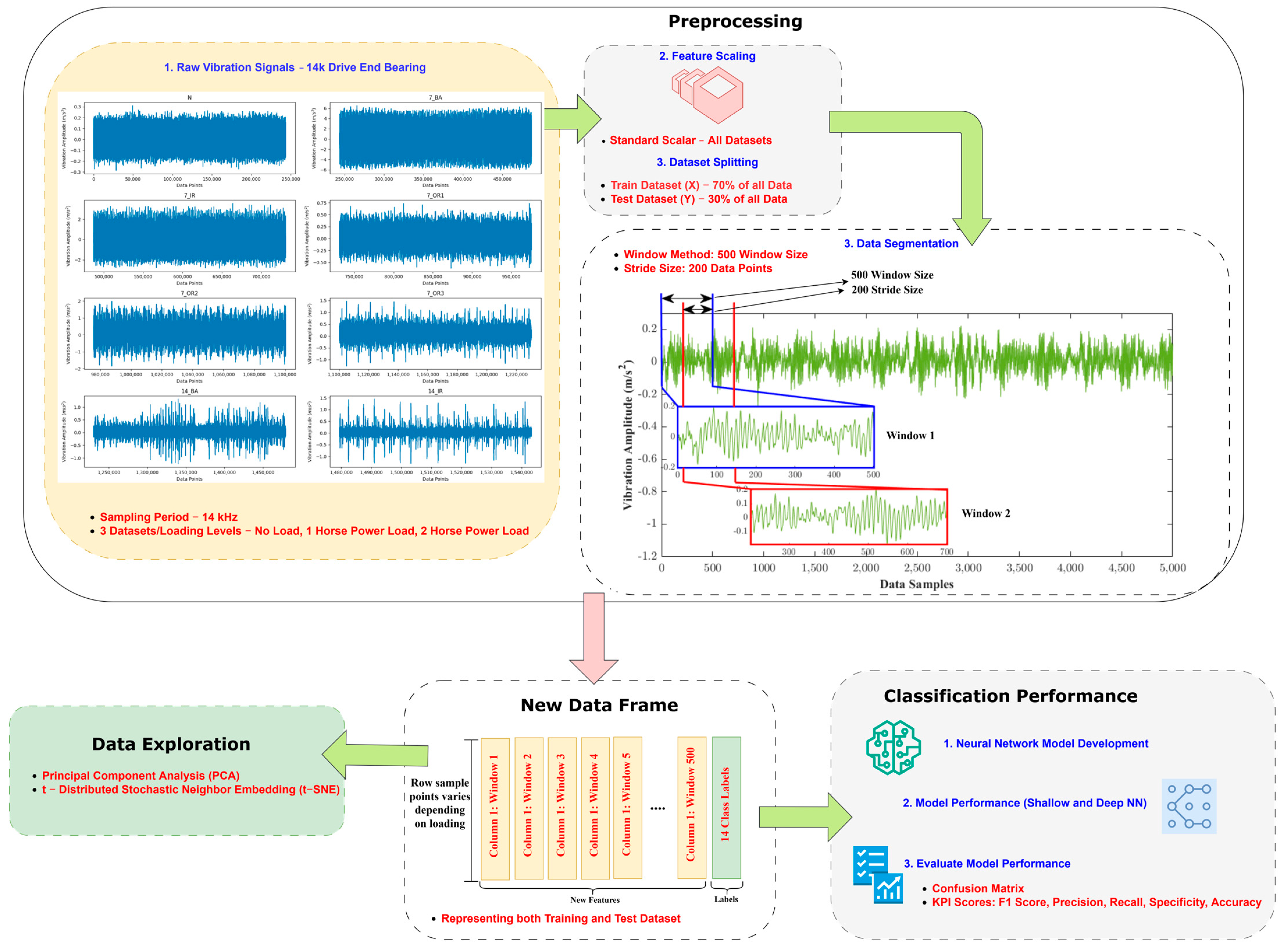
4. Methodology—Fault Diagnosis

Figure 3 illustrates the methodology used to address the research question of developing a fault-classification model for drive-end bearings using raw experimental data from CWRU. To ensure the validity of the study, the data were normalized using the Standard Scalar methodology. To prevent the “Similarity Bias Problem”, as explained in [15], the entire dataset was divided into a training set of 70% and a testing set of 30%. A validation dataset of 20% was grabbed from the training points themselves. This was conducted prior to the window-segmentation methodology. The training and testing data were segmented separately using a window size of 500 and a stride of 200. Feature relationships were visualized using PCA and t-SNE during data exploration. To ensure robust model performance, the data were divided into training, validation, and test sets. Classification models were developed using Python, and pre-built models from MATLAB (version r2023b)’s Classification Learner App were utilized for fault classification, allowing for model comparison and selection.

Figure 3. Bearing-fault diagnosis methodology.

The validation and prediction accuracy results of all the trained models were tabulated, and meaningful conclusions were drawn by evaluating the model’s best and most robust key performance indicators (KPIs) to assess the classification model’s performance. Finally, the methodology adhered to established standards and best practices in machine learning and signal processing to ensure the results’ accuracy, reliability, and validity.

Data Division Representation

In this study, three distinct loading datasets were analyzed, each initially comprising total data points as follows: 2,782,629 for (0 hp), 6,816,994 for (1 hp), and 6,816,996 for (2 hp), as outlined in Table 1. Analyzing each loading condition individually is crucial for accurately determining distinct failure characteristics and improving fault-diagnosis precision, as different loading conditions cause variations in mechanical stress and operational strain. This strategy allows for the construction of more precise predictive models tailored to specific operational conditions, rather than a one-size-fits-all model that might overlook subtle yet critical differences. Furthermore, the proposed approach ensures that the statistical integrity of the analysis is maintained, as combining data from all conditions could violate assumptions like homogeneity of variance, leading to potentially misleading conclusions. Thus, by focusing on each loading condition independently, this study aims to provide detailed insights into bearing behavior under varying operational stresses, offering valuable information for predictive maintenance and fault prevention in industrial machinery.

In terms of data division, 70% was allocated to the training set and 30% was for the test set. Post-segmentation, the data points were distributed as follows: for the (0 hp) load, 19,457,560 data points were assigned to training and 834,669 were assigned to testing; for the (1 hp) load, 4,771,895 were assigned to training and 2,045,099 were assigned to testing; and similarly, for the (2 hp) load, 4,771,897 were allocated to training and 2,045,099 were assigned to testing.

Table 2 displays the results of the segmentation of the training and testing datasets—a process meticulously carried out to improve the model’s ability to generalize from the data. By using a window size of 500 and a stride of 200, the datasets were transformed into segments that offer a structured view of the time-series data, capturing essential temporal features. This process greatly increased the granularity of the analysis, enabling more detailed and accurate modeling of fault conditions across various loads. Once segmented, the distribution of data points was recorded and is presented in the subsequent table.

Table 2. Segmented training, validation, and testing data points across labels for all three loading datasets.

Fault Labels	Load 0			Load 1			Load 2
	Training	Validation	Test	Training	Validation	Test	Training	Validation	Test
N	680	170	362	1359	338	724	1359	338	724
7_BA	681	167	364	1361	337	730	1367	337	732
14_BA	698	172	370	1362	339	730	1362	337	729
21_BA	680	169	365	1363	338	730	1378	342	731
7_IR	680	170	364	1356	339	726	1355	341	727
14_IR	177	43	370	1362	343	729	1358	337	725
21_IR	681	169	366	1376	344	732	1361	337	730
7_OR1	683	169	366	1363	338	727	1366	340	728
7_OR2	347	85	185	1356	339	728	1357	339	729
7_OR3	362	88	194	1353	335	722	1355	338	724
14_OR1	684	171	364	1360	337	731	1362	340	734
21_OR1	688	169	368	1363	338	732	1366	339	734
21_OR2	359	88	191	1365	338	728	1354	338	724
21_OR3	363	90	194	1360	339	729	1359	339	724
Total:	7763	1920	4423	19,059	4742	10,198	19,059	4742	10,195

Additionally, 20% of the training data was kept aside to generalize the model as a validation set. This separation within the training data itself allows for the continuous evaluation of the model’s performance and stability before testing, ensuring that the model does not overfit the training data and can generalize well to new, unseen data. In summary, Table 2 clearly illustrates that all 14 classes are consistently represented across the training, validation, and test sets of each loading dataset.

5. Data Exploration

The following section of this study will examine the exploratory data analysis of the bearing data, utilizing powerful tools such as PCA and t-SNE. Through these techniques, we will uncover the underlying patterns and structure of the data and visualize them intuitively and insightfully. This analysis will provide valuable insights into the relationships and correlations between the different variables, paving the way for further analysis and interpretation.

5.1. Raw Accelerometer Data Exploration

When it comes to visualizing raw data, particularly if it involves time series or measurements across a sequence of data points, the choice of representation depends on the nature of the data and the intended message. In this instance, the raw plots in Figure 4 comprise points sampled from every 100th data point of the data frame, and they are displayed through a scatter plot with a customized color palette to differentiate between various “fault” categories. This method can work well for highlighting specific patterns or anomalies within data.

Figure 4. (a–c). Raw accelerometer data scatter representation revealing the behavior of 14 fault class severities in bearing components for three loading scenarios. (a) Loading Level—0 hp. (b) Loading Level—1 hp. (c) Loading Level—2 hp.

The raw data scatter plots show that the “N” (normal) bearing exhibited consistently low vibration across all loading levels. In contrast, the “7_BA” (0.007 inch roller-element fault) bearing showed significantly higher vibration spikes during the no-load scenario. However, these spikes were not as prominent when the motor was subjected to a load. It is possible that the reason for the difference in vibration spikes between the no-load scenario and the loaded scenarios is due to the change in the operating conditions of the motor. In a no-load scenario, the motor operates with little to no external load applied, which can result in higher vibration levels due to the lack of damping forces. This can make it easier for faults in the roller elements to manifest as noticeable spikes in the vibration data. In contrast, when the motor is loaded, the roller elements may be subjected to different types and magnitudes of forces, resulting in different vibration signatures. It is important to note that further analysis is necessary to fully understand the root cause of these vibration spikes and potential faults in the roller elements.

Above all, the major observation concerns the fault labels with the largest depth damage of 0.021 inches (21_BA, 21_IR, 21_OR1, 21_OR2, 21_OR3). Notably, these labels exhibit prominent vibration spikes that make it easier to identify them as faulty, irrespective of the loading scenario. In contrast, fault labels with depths of 0.014 and 0.007 inches are not easily identifiable based on vibration spikes alone. A possible explanation for this could be that the fault with the largest depth damage is located in a critical location of the bearing or motor system. Certain areas of a bearing or motor system may be more susceptible to generating larger vibrations due to their proximity to other components or the way forces are distributed within the system. If the fault with the largest depth damage is in a critical location, this could explain the larger vibration spikes. Additionally, the simple reason is that faults with larger depth damage may have a greater impact on the natural frequencies of the bearing system. The natural frequencies of the system depend on the stiffness and mass properties of the system, which can be affected by the presence of faults. A fault with larger depth damage may change the stiffness and mass properties of the bearing system more significantly, resulting in larger shifts in natural frequencies and corresponding vibration spikes.

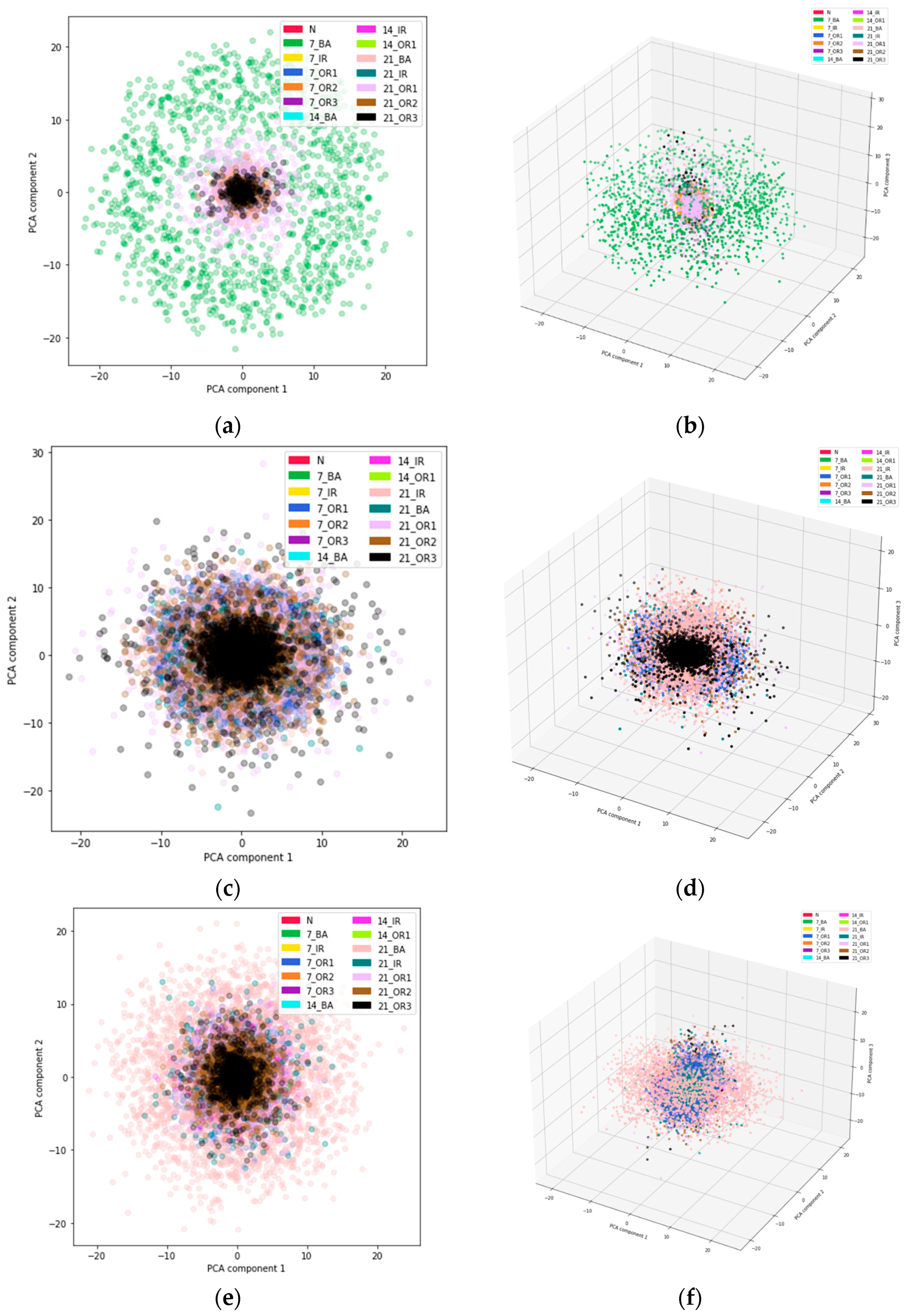
5.2. Principal Component Analysis (PCA)

PCA is a variable reduction procedure similar to factor analysis and uses linear combinations of the original correlated measurements to arrive at a new coordinate system. In this new coordinate system, the first principal component accounts for the largest variances in the data, and other principal components account for progressively smaller amounts of variance [16,17]. The principal components are uncorrelated with each other, and they are orthogonal to each other, meaning that they are perpendicular in the n-dimensional space of the original data [18]. This study will utilize this procedure for exploratory analysis purposes only.

When analyzing the geometry of a dataset using PCA, the resulting 2D and 3D plots can reveal important information about the structure of the data in the case of the CWRU bearing dataset analyzed. Figure 5a shows that one particular class label’s data point—7_BA—is projected in a circular motion, while the other 13 label data points are not distinguishable as they are clustered together in between the 7_BA label data point’s circular projection. The 3D PCA view in Figure 5b presents similar results even with the additional principal component. This finding suggests that class 7_BA, with the circular data point projection in the PCA plot, has a unique pattern of variation that distinguishes it from the other classes. The circular motion implies a strong circular relationship among the variables within this category, signifying high correlations and joint variations in a circular pattern. This circular pattern may stem from various factors, including the inherent characteristics of the data, the instrumentation employed for measurements, or the underlying physical processes under investigation.

Figure 5. PCA projections of: (a) 0 hp Load 2D PCA, (b) 0 hp Load 3D PCA, (c) 1 hp Load 3D PCA, (d) 1 hp Load 2D PCA, (e) 2 hp Load 2D PCA, (f) 2 hp Load 3D PCA.

Visualizing the PCA projections of the data under the two loading levels in Figure 5c–f, it was found that the fault class labels with the largest depth faults (21_BA, 21_IR, 21_OR1, 21_OR2, and 21_OR3) are distinguishable in the 2D PCA plot, while the other fault class labels with lower fault depths are clustered behind the larger ones. Furthermore, in the 3D PCA plot, there were no new projection patterns that emerged beyond those already observed in the 2D plots. This finding suggests that the fault class labels with larger fault depths have a unique pattern of variation that distinguishes them from the other fault class labels. This could be because the faults with larger depths involve more significant changes in the underlying physical or geological processes, resulting in more distinct patterns of variation in the data. On the other hand, the fault class labels with lower fault depths may not exhibit as much variation or may be more difficult to distinguish from each other due to their relatively minor impact on the underlying processes.

Additionally, the data geometry analysis of the dataset with three loading levels revealed that the PCA technique was not able to separate the normal class from the fault class labels effectively. This implies that the variation within the normal class and fault class labels is not distinct enough to be separated by the PCA method.

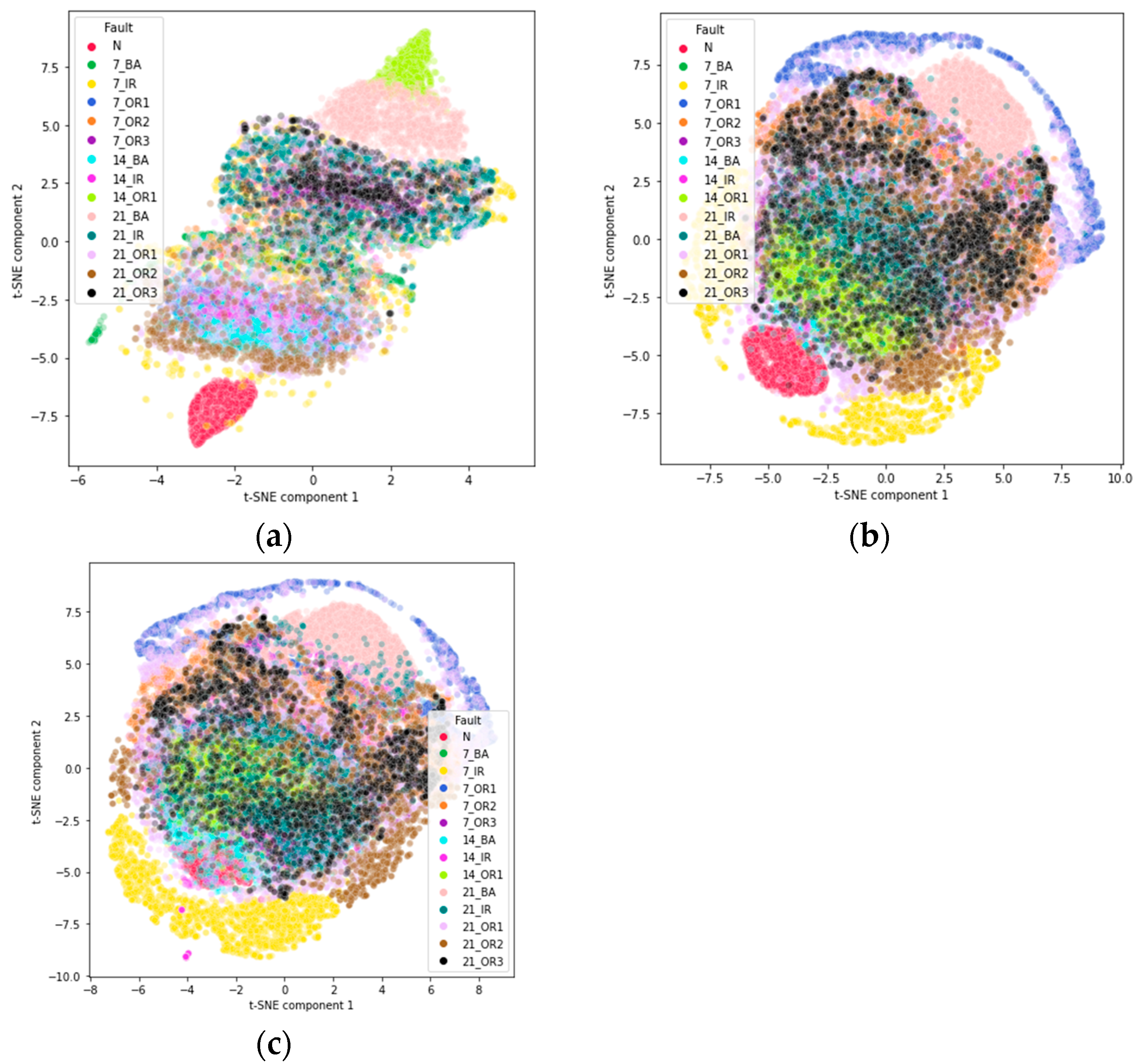
5.3. t-Distributed Stochastic Neighbor Embedding (t-SNE)

t-SNE is an ML algorithm used for data visualization and dimensionality reduction. This procedure is often used to display high-dimensional data in a low-dimensional space, such as a 2D plot, to provide better insight into the data point’s relationship. t-SNE models each high-dimensional object through probability distribution in a low-dimensional space [19]. Then, it tries to find mapping options between the two spaces that preserve the similarities between objects. A cost function is optimized that measures the difference between the pairwise similarities of objects in the high-dimensional space and their counterparts in the low-dimensional space. In this research, we explore the potential of t-SNE compared to PCA.

The exploration in Figure 6 suggests that the underlying structure of the data may be complex, with multiple overlapping patterns of variation that are difficult to distinguish using t-SNE. It is possible that there are multiple factors driving the observed variation in the data, such as differences in operating conditions. These factors may be difficult to fully capture using t-SNE, which relies on the assumption of a low-dimensional structure within the data. Furthermore, t-SNE is known to be a relatively weak technique for distinguishing between classes within a dataset. This is because t-SNE is primarily designed to preserve the local relationships between data points rather than the global relationships between classes. As a result, it may not be the best technique for distinguishing between closely related classes, such as those within the current bearing dataset.

Figure 6. t-SNE analysis on bearing dataset: (a) t-SNE on 0 hp data, (b) t-SNE on 1 hp data, (c) t-SNE on 2 hp data.

6. Model Description

The following section provides an overview of classifier models and their hyperparameters in two families: neural network-based and non-neural network-based. Classifier models are widely used in machine learning for categorizing data points into different classes based on specific features or attributes. Hyperparameters are a crucial component of machine learning models; they are set before training and significantly impact the model’s performance. This section delves into various types of classifier models, their architectures, and the hyperparameters used and tuned to improve their classification performance. In addition, this section highlights the impact of these hyperparameters on the model’s performance and explores some of the commonly used techniques for optimizing them.

6.1. Multi-Layer Perceptron (MLP)

MLP is a feedforward neural network that is widely used for classification tasks. It consists of multiple layers of interconnected nodes or neurons, where each neuron receives inputs from the previous layer and applies a nonlinear activation function to produce an output. MLP can be trained using backpropagation with gradient descent optimization. The hyperparameters and functions are tabulated in Table 3 below.

Table 3. Classification Model Specification List.

Model Label	Classifier	Specification
MLP	MLP NN	Architecture: (1024IN—ReLU |512DL—ReLU|256DL—ReLU|14OUT—Softmax|Optimizer: adam|Loss: categorical_crossentropy)
Bidirectional LSTM	Bi-LSTM	Architecture: [1BL—LSTM, 128 Units, Return Sequences: True, Input Shape: Specified], [1DO—Dropout, Rate: 0.2], [1FD—Dense, 32 Units, Activation: tanh], [2BL—LSTM, 64 Units, Return Sequences: False], [2DO—Dropout, Rate: 0.1], [1FD—Dense, 16 Units, Activation: tanh], [1FD—Dense, 256 Units, Activation: relu], [2FD—Dense, Number of Classes, Activation: Softmax], Optimizer: adam, Loss: categorical_crossentropy. Metrics: accuracy
Deep LSTM	D-LSTM	Architecture: [1LD—LSTM, 64 Units, Return Sequences: True, Input Shape: Specified], [1DO—Dropout, Rate: 0.2], [2LD—LSTM, 32 Units, Return Sequences: False], [2DO—Dropout, Rate: 0.2], [1FD—Dense, 32 Units, Activation: ReLU], [2FD—Dense, Number of Classes, Activation: Softmax], Optimizer: adam, Loss: categorical_crossentropy. Metrics: accuracy
1D-CNN	1D Convolutional NN	Architecture: ([1Fd—Conv1D, 64 Filters, 100 Kernels, Activation: ReLU]|[2FD—Conv1D, 32 Filters, 50 Kernels, Activation: ReLU]|1FL|[1PL—4 MaxPooling1D]|[1FC—100 Dense, Activation: ReLU]|Optimizer: adam|Loss: categorical_crossentropy)
MK-CNN	1D Multi Kernel CNN	Architecture 1: ([1Fd—Conv1D, 64 Filters, 200 Kernels, Activation: ReLU, 0.5 Dropout, 1PL—20 MaxPooling1D, 1FL—Flatten]| Architecture 2: ([1Fd—Conv1D, 64 Filters, 100 Kernels, Activation: ReLU, 0.5 Dropout, 1PL—10 MaxPooling1D, 1FL—Flatten]| Architecture 3: ([1Fd—Conv1D, 64 Filters, 50 Kernels, Activation: ReLU, 0.5 Dropout, 1PL—5 MaxPooling1D, 1FL—Flatten])| [1DL—100 layers, Activation: ReLU]|[1OUT—Activation: Softmax]|Optimizer: adam|Loss: categorical_crossentropy)
2D-CNN	2D CNN	Architecture: Sequential|([1FD—Conv2D, 32 Filters, Kernel size (3, 3), Activation: ReLU]|[1PL— MaxPooling2D (2, 2), Strides (2, 2)]|[1CL—64 Conv2D, Kernel size (3, 3), Activation: ReLU]|[1PL—MaxPooling2D (2, 2), Strides (2, 2)]|[1DL—128 layers, Activation: ReLU]|[1OUT—Activation: Softmax]|Optimizer: adam|Loss: categorical_crossentropy)

Note: DL: filters in the dense layer, FC: neurons in a fully connected layer: (size), BL: Bidirectional layer, OUT: neurons in the output layer, IN: input layer, Fd: Feature Detector, PL: Pooling Layer, FL: Flatten Layer, CL: Convolutional Layer, LD: “LSTM Dense” layer, DO: “Dropout”, FD: Fully Connected (Dense) layer.

6.2. Recurrent Neural Network

The long short-term memory (LSTM) model, a variant of recurrent neural networks, has been increasingly recognized for its proficiency in handling time-series data, as noted in critical studies [20,21]. The research focuses on two types of RNN, namely deep LSTM and bidirectional LSTM. These RNNs excel in capturing the temporal dependencies and complexities present in sequential data, making them a great fit for our application in fault classification in bearing components using raw accelerometer data.

• Deep LSTM: This model stacks multiple LSTM layers to create a deeper network architecture. This setup allows the model to learn higher-level temporal representations at each layer, making it more robust and accurate. This is particularly beneficial for complex time-series prediction tasks, where long-range dependencies and patterns are important. Each LSTM layer captures different aspects of the temporal data, and the deep architecture usually ends with a fully connected layer that maps the final LSTM layer’s output to the desired output shape. This could be a specific number of classes for classification tasks. Deep LSTMs are typically trained using backpropagation through time (BPTT) and are often optimized with algorithms such as Adam or RMSprop, leveraging the categorical cross-entropy loss function for classification problems.
• Bidirectional LSTM (Bi-LSTM): Bi-LSTM networks enhance the standard LSTM by introducing another layer that processes the input sequence in reverse. This allows Bi-LSTMs to capture dependencies from both past and future contexts, resulting in a more comprehensive understanding of the sequence. This architecture is particularly useful for tasks where comprehending each part requires understanding the entire sequence’s context, such as natural language processing and speech recognition. In Bi-LSTMs, the forward and backward LSTM layers run parallel to each other, and their outputs are combined at each time step through concatenation or summing. This combined output is then passed through additional layers or directly to the output layer, depending on the complexity of the task. Bi-LSTM networks also benefit from deep learning optimizations and loss functions like deep LSTMs, ensuring effective training and convergence for various sequence modeling tasks.

6.3. Convolutional Neural Network

A CNN is a type of neural network particularly suited for image classification tasks. It consists of multiple convolutional layers, which apply a set of learnable filters to the input image, followed by pooling layers to reduce the spatial dimensions of the feature maps. The output of the last convolutional layer is typically flattened and fed into a fully connected layer for classification. Three powerful variances of CNN have been developed and used to classify faults using the raw accelerometer data in this research article; its architecture is represented in Figure 7 below.

Figure 7. Three-variant CNN architecture schematic.

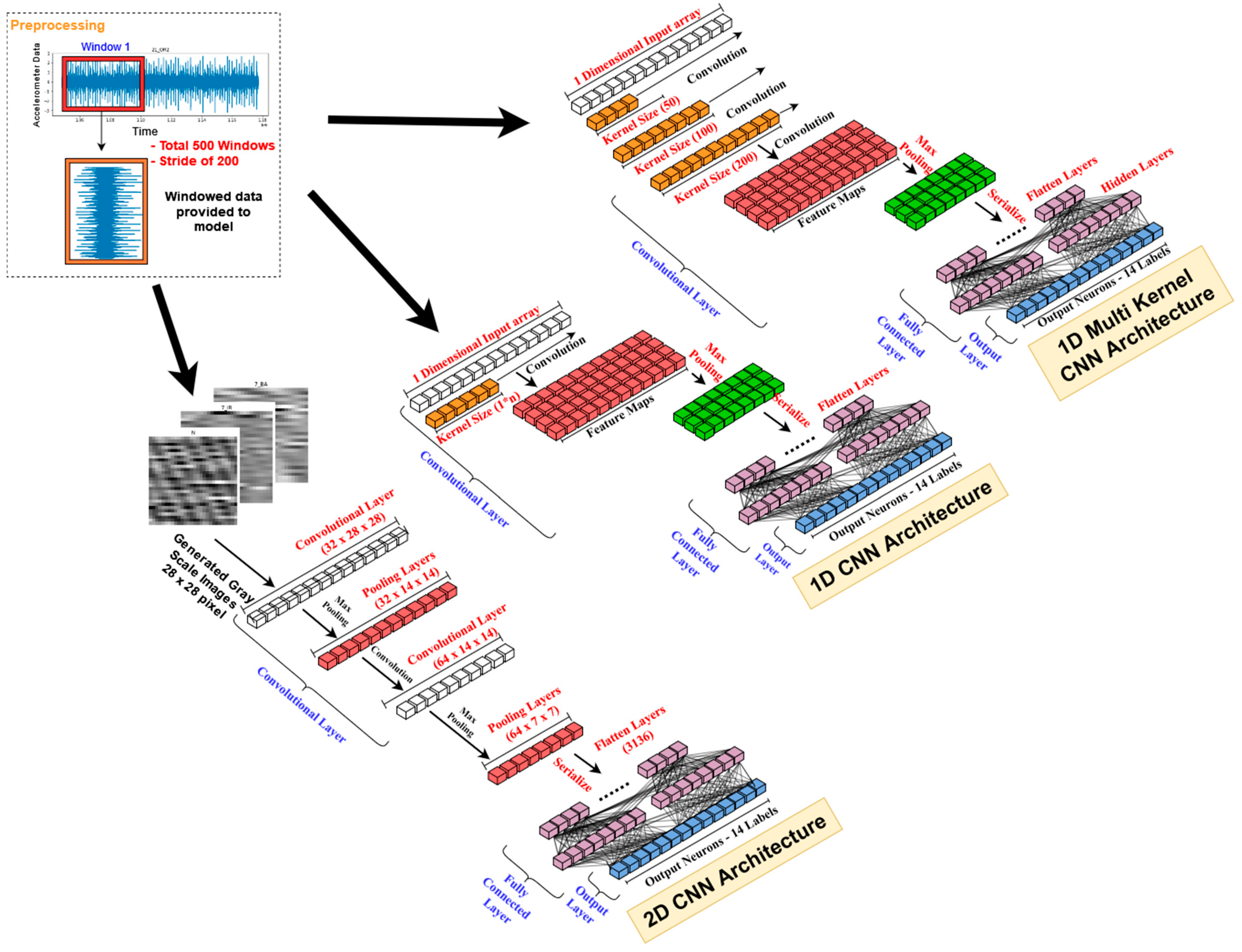
• One-dimensional CNN (1D-CNN): supervised learning algorithm used mainly for processing data sequences such as time series, text, and speech. A set of learnable filters is applied to the input, which is this configuration is a one-dimensional sequence of values [22]. The architecture consists of a 1D convolutional layer, each followed by a max pooling layer to reduce the spatial dimensions of the feature map. A flattened output is then passed through a fully connected layer with 100 units, following a final output layer with SoftMax activation to produce a probability distribution of the input belonging to each of the 14 classes. The categorical cross-entropy loss function is used to train the model and optimized using the Adam optimizer.
• Multi Kernel 1D-CNN: This is the second CNN variant developed with three different input signals processed through three separate 1D convolutional layers. Each 1D convolutional layer has been assigned different kernel sizes of 200, 100, and 50. Each layer is followed by a max pooling layer to reduce the spatial dimensions of the feature maps. The resulting feature maps are flattened and concatenated, then passed through a fully connected layer with 100 units and a final output layer with a SoftMax activation function to produce the probability distribution of the input belonging to each class. The model is trained using the categorical cross-entropy loss function and the Adam optimizer.
• Two-dimensional (2D) CNN: In this model, raw accelerometer signals are first transformed into 28 × 28 pixel grayscale images for each class’s points. The 2D-CNN consists of two convolutional layers, each followed by a max pooling layer to down-sample the feature maps. The first convolutional layer has 32 filters with a kernel size of 3 × 3, while the second layer has 64 filters with the same kernel size and activation function ReLU. The padding parameter is set to “same” to ensure that the output feature maps have the exact spatial dimensions as the input. The output of the last max pooling layer is flattened and passed through two dense layers with 128 and 14 neurons, respectively. The activation function used for these layers is ReLU. Finally, the output layer uses the SoftMax activation function to predict the probability of each class. By using a 2D CNN, the model can capture spatial correlations between adjacent pixels in the grayscale images, which can be helpful in detecting patterns in the accelerometer raw signals [23,24].

7. Results

It is essential to comprehend the significance of the various metrics used to assess the performance of machine learning models before delving into the detailed metrics in our study. These metrics, including specificity, F1-score, recall, and precision, provide an understanding of the model’s efficiency and highlight strengths and areas for improvement. In Section 7.1, works on the application of these metrics to analyze classifier performance are elaborated relating to the CWRU bearing dataset. This evaluation is instrumental in comprehending the abilities of both non-neural and neural network-based classifiers in processing raw data, which is a crucial aspect of our study. Through this analysis, we aim to provide a comprehensive overview of each model’s effectiveness when applied directly to unprocessed datasets, paving the way for a detailed exploration of their performance.

7.1. Recall, Sensitivity, F1-Score and Precision

Accuracy, F1-score, recall, and precision are common evaluation metrics used in classification tasks to measure the performance of a machine learning model [25]. A brief description of each of these metrics is listed below:

○

Accuracy: measures the percentage of correctly classified instances by a model out of the total number of instances. It is calculated as the ratio of the number of correctly classified instances to the total number of instances, as per the formula below:

$$Accuracy=\frac{(Tp+Tn)}{(Tp+Tn+Fp+Fn)}$$

(1)

○

Recall: is the proportion of true-positive instances (i.e., instances correctly classified as positive) out of the total number of positive instances. It is calculated as the ratio of true-positive instances to the sum of true-positive and false-negative instances.

$$Recall=\frac{Tp}{(Tp+Fn)}$$

(2)

○

Precision: is the proportion of true-positive instances out of the total number of instances the model classified as positive. It is calculated as the ratio of true-positive instances to the sum of true-positive and false-positive instances.

$$Precision=\frac{Tp}{(Tp+Fp)}$$

(3)

○

F1-score: is a measure of the harmonic mean between precision and recall. It is a more informative metric than accuracy in situations with a class imbalance in the data, i.e., when the number of instances in one class is much larger than the other. The F1-score considers both the precision and recall of a model and is calculated as the harmonic mean of these two metrics.

$$F1 score=\frac{2\left(Precision\times Recall\right)}{\left(Precision+Recall\right)}$$

(4)

○

Specificity: also referred to as the true-negative rate, calculates the ratio of actual negatives that are correctly identified as negatives. For instance, it measures the percentage of healthy individuals who are correctly identified as not having the condition in a medical test. It is a key metric in evaluating the performance of a classification model, especially in imbalanced datasets or when the cost of false negatives is high.

$$Specificity=\frac{Tn}{\left(Tn+Fp\right)}$$

(5)

Note: $Tp$—True Positive, $Tn$—True Negative, $Fn$—False Negative, $Fp$—False Positive.

In the present study, we have utilized a variety of classification models, both non-neural and neural, to analyze the CWRU bearing dataset. It is worth noting that our approach involved using the raw datasets, with only normalization and segmentation procedures applied, as input for training the selected models provided in Table 3. This approach is distinct from previous works, which commonly employ feature engineering, dimensionality reduction, and other preprocessing steps prior to classification analysis. We aimed to explore the effectiveness of using raw data directly in classification tasks and to compare the performance of different models under this approach.

Upon examining the results obtained, we observed that several classifiers, such as Fine Tree, Naïve Bayes, Linear Discriminant, Quadratic Discriminant, and Medium Tree, demonstrated poor performance in accurately classifying the CWRU bearing class labels, with average prediction accuracy under 35% in all loading levels; hence, these results were not placed in the paper. There are several possible hypotheses as to why these classifiers may have performed poorly. Fine Tree is a decision tree-based algorithm that may struggle to handle complex and noisy data, which could potentially result in the overfitting or underfitting of the model. Linear Discriminant and Quadratic Discriminant are based on a statistical approach that assumes the input data is normally distributed, which may not hold true in the case of the CWRU bearing dataset. This assumption violation can negatively affect the performance of these classifiers. A Medium Tree is a variation of decision trees and is also susceptible to overfitting when applied to high-dimensional datasets with large numbers of features. Therefore, through the evaluation of these classifiers, we understand it is essential to analyze the characteristics of the dataset and choose an appropriate classifier that can effectively capture the underlying patterns and relationships in the data whilst avoiding issues of overfitting and underfitting to achieve satisfactory classification results.

Furthermore, shallow and deep models of the NN family were experimented upon, where a relatively high classification accuracy above 85% was recorded in the RNN and CNN variant architectures. Although MLP is a fundamental architecture in neural networks, it may not be as effective as RNN and CNN variants in classifying the CWRU bearing dataset due to its limitations in processing sequential or spatial data. MLPs are networks that are fully connected and excel at capturing linear relationships between inputs and outputs. However, they lack the ability to model the temporal dependencies and spatial patterns that are inherent in time-series or image data. This limitation is particularly important in applications like the CWRU dataset analysis, where the data are inherently sequential (bearing vibration signals) or spatial (transformed accelerometer signals into images for CNN analysis).

RNNs are neural networks that have recurrent connections, allowing them to retain information from previous inputs. As a result, they are particularly useful for time-series data since they can capture temporal dependencies. This ability enables RNNs to comprehend the order of events in vibration signals, which is crucial for precise fault classification in bearings. On the other hand, CNNs are designed to recognize spatial patterns by using convolutional filters, making them exceptionally effective for tasks that involve the spatial arrangement of data points, such as pixels in an image or patterns in a signal transformed into a 2D representation.

In contrast, MLP models treat input features independently, ignoring the order or spatial arrangement, which can lead to a significant loss of information critical for making accurate predictions in such datasets. Consequently, while MLPs serve as a strong baseline for many classification tasks, their structure inherently limits their effectiveness in tasks requiring an understanding of temporal sequences or spatial patterns, leading to their lower performance compared to RNNs and CNNs in this context.

The optimal performance of the models relied heavily on tuning the hyperparameters. In order to achieve greater classification accuracy, it is essential to conduct a hyperparameter search using techniques like “random search” and “Bayesian optimizer”. The models employed in this study were deep neural network architectures, including D-LSTM, Bi-LSTM, 1D-CNN, MK-CNN, and 2D-CNN. The specifications and hyper-parameters for all the tested models are presented in detail in Table 3. The test accuracies for all the different NN models were calculated using Equation (1), and they ranged from 70% to 99%, as shown in Table 4. Several factors contributed to the success of these models; notably, their flexibility allows them to capture complex patterns and relationships within the accelerometer dataset. The deeper architectures of these models allow for the extraction of more abstract features, enabling better discrimination between different classes. In particular, the convolutional layers in CNNs are designed to identify spatial and temporal patterns in data, making them well-suited for tasks like sequential data and image classification. Additionally, the careful tuning of hyperparameters, such as learning rate, number of layers, and number of filters, can lead to better model performance. The best result of all was certainly shown by the 2D-CNN classifier. The accelerometer data transformed into grayscale images allowed the CNN to learn spatial patterns in the images, which can be used to distinguish between different class labels. The 14 class labels captured in imaging allowed the model to learn different levels of abstraction, from low-level features such as edges and corners to high-level features such as shapes and patterns. Additionally, the proper tuning of the hyperparameters of the learning rate, batch sizing, and epoch count established a robust network for classifying raw accelerometer signals.

Table 4. Results of Validation and Test Accuracy for the Classification Models.

Classifier	Validation Accuracy (%)			Test Accuracy (%)
	0 hp	1 hp	2 hp	0 hp	1 hp	2 hp
MLP	73.94	55.74	51.3	68.38	55.73	54.66
D-LSTM	81.32	81.51	78.93	70.50	81.50	82.54
Bi-LSTM	89.84	81.90	80.33	78.96	81.89	81.70
1D-CNN	90.26	89.14	89.2	85.02	89.27	90.30
Mk-CNN	95.72	92.36	90.67	94.26	91.87	93.44
2D-CNN	98.40	93.62	95.63	99.32	91.16	94.97

Table 4 shows that the 2D-CNN model consistently outperforms DNNs for all three load levels. Figure 8 displays confusion matrices for all three load settings to provide a closer look at its test accuracy performance, These matrices reveal positive signs for classifying bearing states. High values along the diagonal (true positives) indicate good identification of both normal and faulty conditions. However, there are some interesting differences depending on the load.

Figure 8. Confusion matrix projection of the 2D-CNN model performance (a) 0 hp accuracy plot, (b) 1 hp accuracy plot, (c) 2 hp accuracy plot.

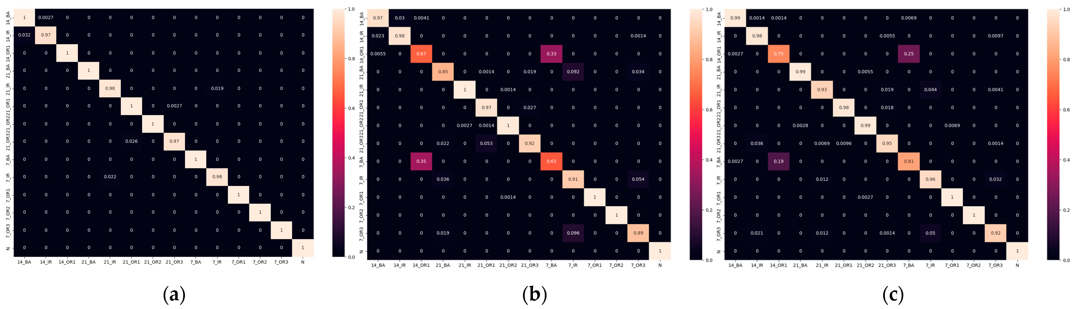
• No-Load: The model achieves near-perfect accuracy for most classes, suggesting strong discriminative power despite the absence of load-induced stress signatures. Minimal off-diagonal values indicate a low number of false positives.
• Loaded Conditions: Both the 1 hp and 2 hp scenarios show a slight increase in misclassifications (higher off-diagonal values) compared to the no-load model. This suggests the model struggles to differentiate between certain fault types, possibly due to inherent data complexity or similar signatures under load.
• Impact of Load: Increased load introduces a trade-off. While the model maintains good accuracy for some fault types and the normal state, others exhibit lower precision under higher loads. This highlights the varying influence of load on different fault signatures.

Figure 9 illustrates the accuracy prediction behavior for each model in the three loading levels. It can be hypothesized that the accuracy of all models decreased gradually as the loading increased. This could be due to the rise in complexity of the accelerometer spikes due to changes in the loading level. However, deep NN models were able to preserve their high percentage accuracy even with the change in loading. The KPIs for the deep NN models were further calculated and are tabulated in Table 5 to support the justifications made previously.

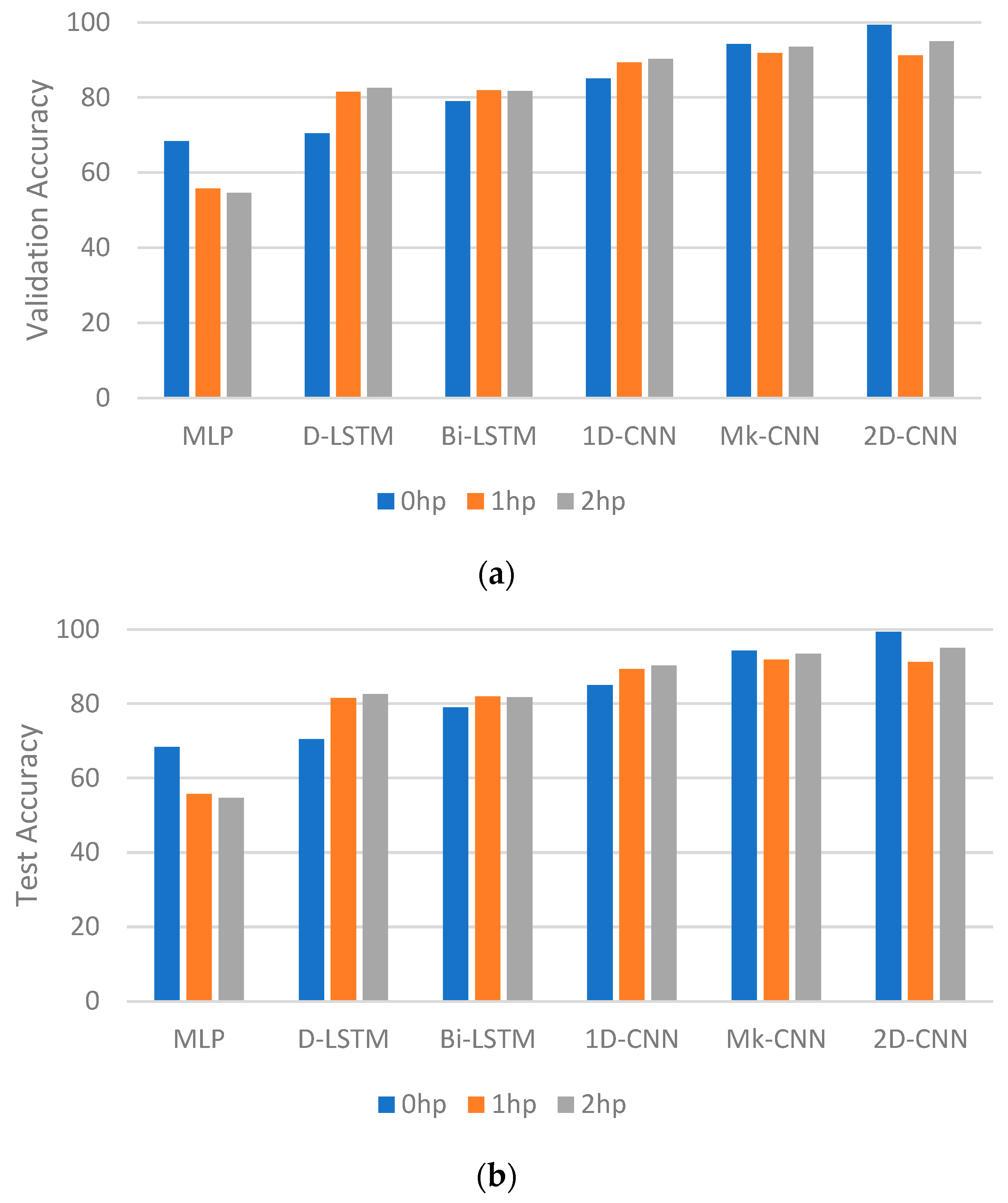
Figure 9. Performance evaluation classifier models under the three loading levels (a) Classifier validation accuracy, (b) Classifier test accuracy.

Table 5. KPI evaluation of the best classifiers.

Classifier	Loading	KPI
		Precision	Specificity	Recall	F1-Score
MLP	0 hp	0.693	0.975	0.683	0.685
	1 hp	0.565	0.966	0.557	0.558
	2 hp	0.534	0.914	0.545	0.551
D_LSTM	0 hp	0.615	0.977	0.705	0.638
	1 hp	0.735	0.985	0.815	0.763
	2 hp	0.843	0.983	0.8253	0.8115
Bi-LSTM	0 hp	0.6902	0.983	0.789	0.724
	1 hp	0.816	0.915	0.892	0.813
	2 hp	0.865	0.923	0.817	0.821
1D-CNN	0 hp	0.865	0.988	0.850	0.846
	1 hp	0.897	0.991	0.983	0.892
	2 hp	0.863	0.964	0.902	0.876
MK-CNN	0 hp	0.942	0.995	0.942	0.940
	1 hp	0.915	0.895	0.9167	0.882
	2 hp	0.923	0.996	0.932	0.910
2D-CNN	0 hp	0.993	0.999	0.993	0.998
	1 hp	0.913	0.993	0.911	0.910
	2 hp	0.950	0.996	0.949	0.949

8. Conclusions and Remarks

This paper proposed a methodology for the efficient fault classification of bearing-related faults. A variety of classification models, both non-neural and neural, were utilized to analyze the CWRU bearing dataset. It is important to note that the performance of a classifier can be heavily dependent on the specific dataset being analyzed and the characteristics of the data. While some classifiers may perform poorly on a given dataset, others may exhibit superior performance. Therefore, it is crucial to thoroughly evaluate the performance of multiple classifiers to determine the optimal algorithm for a specific classification task.

It is worth noting that our approach involved using raw datasets, with only normalization and segmentation procedures applied, as input for training the selected models. This approach is distinct from previous works, which commonly employ feature engineering, dimensionality reduction, and other preprocessing steps prior to classification analysis. The proposed methodology had practical implications for predictive maintenance and contributed to the field of machine learning by demonstrating the effectiveness of using raw accelerometer signals for fault classification.

Future research could delve into integrating this methodology with real-time monitoring systems, harnessing the capabilities of IoT and edge computing. By doing so, we can create more dynamic and responsive fault-detection mechanisms in industrial settings. Additionally, the proposed deep neural network (DNN) models will undergo further enhancements to classify all forms of bearing failure, taking into account the specific loading level state of the machine.

References

- Kompella, K.C.D.; Rao, M.V.G.; Rao, R.S. Bearing fault detection in a 3 phase induction motor using stator current frequency spectral subtraction with various wavelet decomposition techniques. Ain Shams Eng. J. 2018, 9, 2427–2439. [Google Scholar] [CrossRef]
- Morris, D.; Sadeghi, F.; Singh, K.; Voothaluru, R. Residual stress formation and stability in bearing steels due to fatigue induced retained austenite transformation. Int. J. Fatigue 2020, 136, 105610. [Google Scholar] [CrossRef]
- Rajabi, S.; Azari, M.S.; Santini, S.; Flammini, F. Fault diagnosis in industrial rotating equipment based on permutation entropy, signal processing and multi-output neuro-fuzzy classifier. Expert. Syst. Appl. 2022, 206, 117754. [Google Scholar] [CrossRef]
- Yang, C.; Ma, J.; Wang, X.; Li, X.; Li, Z.; Luo, T. A novel based-performance degradation indicator RUL prediction model and its application in rolling bearing. ISA Trans. 2022, 121, 349–364. [Google Scholar] [CrossRef] [PubMed]
- Liu, S.; Fan, L. An adaptive prediction approach for rolling bearing remaining useful life based on multistage model with three-source variability. Reliab. Eng. Syst. Saf. 2022, 218, 108182. [Google Scholar] [CrossRef]
- Saha, D.K.; Hoque, M.E.; Badihi, H. Development of Intelligent Fault Diagnosis Technique of Rotary Machine Element Bearing: A Machine Learning Approach. Sensors 2022, 22, 1073. [Google Scholar] [CrossRef] [PubMed]
- Ding, Y.; Jia, M.; Miao, Q.; Cao, Y. A novel time–frequency Transformer based on self–attention mechanism and its application in fault diagnosis of rolling bearings. Mech. Syst. Signal Process 2022, 168, 108616. [Google Scholar] [CrossRef]
- Zhang, S.; Zhang, S.; Wang, B.; Habetler, T.G. Machine Learning and Deep Learning Algorithms for Bearing Fault Diagnostics—A Comprehensive Review. IEEE Access 2020, 8, 29857–29881. [Google Scholar] [CrossRef]
- Lu, C.; Wang, Z.Y.; Qin, W.L.; Ma, J. Fault diagnosis of rotary machinery components using a stacked denoising autoencoder-based health state identification. Signal Process. 2017, 130, 377–388. [Google Scholar] [CrossRef]
- Zhang, T.; Liu, S.; Wei, Y.; Zhang, H. A novel feature adaptive extraction method based on deep learning for bearing fault diagnosis. Measurement 2021, 185, 110030. [Google Scholar] [CrossRef]
- Singh, S.; Kumar, A.; Kumar, N. ScienceDirect Motor Current Signature Analysis for Bearing Fault Detection in Mechanical Systems. Procedia Mater. Sci. 2014, 6, 171–177. [Google Scholar] [CrossRef]
- (PDF) Bearing Fault Diagnosis Using Motor Current Signature Analysis and the Artificial Neural Network. Available online: https://www.researchgate.net/publication/339366382_Bearing_Fault_Diagnosis_Using_Motor_Current_Signature_Analysis_and_the_Artificial_Neural_Network (accessed on 3 April 2023).
- Alonso-González, M.; Díaz, V.G.; Pérez, B.L.; G-Bustelo, B.C.P.; Anzola, J.P. Bearing Fault Diagnosis With Envelope Analysis and Machine Learning Approaches Using CWRU Dataset. IEEE Access 2023, 11, 57796–57805. [Google Scholar] [CrossRef]
- Neupane, D.; Seok, J. Bearing fault detection and diagnosis using case western reserve university dataset with deep learning approaches: A review. IEEE Access 2020, 8, 93155–93178. [Google Scholar] [CrossRef]
- Apparatus & Procedures|Case School of Engineering|Case Western Reserve University. Available online: https://engineering.case.edu/bearingdatacenter/apparatus-and-procedures (accessed on 4 April 2024).
- Jiang, L.; Fu, X.; Cui, J.; Li, Z. Fault detection of rolling element bearing based on principal component analysis. In Proceedings of the 2012 24th Chinese Control and Decision Conference, CCDC 2012, Taiyuan, China, 23–25 May 2012; pp. 2944–2948. [Google Scholar] [CrossRef]
- Mezni, Z.; Delpha, C.; Diallo, D.; Braham, A. Performance of Bearing Ball Defect Classification Based on the Fusion of Selected Statistical Features. Entropy 2022, 24, 1251. [Google Scholar] [CrossRef] [PubMed]
- Raj, K.K.; Joshi, S.H.; Kumar, R. A state-space model for induction machine stator inter-turn fault and its evaluation at low severities by PCA. In Proceedings of the 2021 IEEE Asia-Pacific Conference on Computer Science and Data Engineering, CSDE 2021, Brisbane, Australia, 8–10 December 2021. [Google Scholar] [CrossRef]
- Xu, X.; Xie, Z.; Yang, Z.; Li, D.; Xu, X. A t-SNE Based Classification Approach to Compositional Microbiome Data. Front. Genet. 2020, 11, 1633. [Google Scholar] [CrossRef]
- Tian, H.; Fan, H.; Feng, M.; Cao, R.; Li, D. Fault Diagnosis of Rolling Bearing Based on HPSO Algorithm Optimized CNN-LSTM Neural Network. Sensors 2023, 23, 6508. [Google Scholar] [CrossRef] [PubMed]
- Sun, H.; Zhao, S. Fault Diagnosis for Bearing Based on 1DCNN and LSTM. Shock. Vib. 2021, 2021, 1221462. [Google Scholar] [CrossRef]
- Ince, T.; Malik, J.; Devecioglu, O.C.; Kiranyaz, S.; Avci, O.; Eren, L.; Gabbouj, M. Early Bearing Fault Diagnosis of Rotating Machinery by 1D Self-Organized Operational Neural Networks. IEEE Access 2021, 9, 139260–139270. [Google Scholar] [CrossRef]
- Toma, R.N.; Piltan, F.; Im, K.; Shon, D.; Yoon, T.H.; Yoo, D.S.; Kim, J.M. A Bearing Fault Classification Framework Based on Image Encoding Techniques and a Convolutional Neural Network under Different Operating Conditions. Sensors 2022, 22, 4881. [Google Scholar] [CrossRef] [PubMed]
- Yang, J.; Liu, J.; Xie, J.; Wang, C.; Ding, T. Conditional GAN and 2-D CNN for Bearing Fault Diagnosis with Small Samples. IEEE Trans. Instrum. Meas. 2021, 70, 3525712. [Google Scholar] [CrossRef]
- Alexa, R.Y.A.; Alexa, D.A.A. Probabilistic Extension of Precision, Recall, and F1 Score for More Thorough Evaluation of Classification Models. In Proceedings of the First Workshop on Evaluation and Comparison of NLP Systems, Online, 20 November 2020. [Google Scholar]