1. Introduction
The International Federation of Red Cross (IFRC) defines a disaster as “an event that disrupts the normal functioning conditions of a community and exceeds its ability to deal with the effects with its own resources [
1]”. The term natural risks refers to “natural phenomena that have the potential to cause a disaster, such as climatologist, meteorologist, hydrologist, biological or geophysical phenomena”. Given the natural conditions of the planet, all geographic regions are exposed to different types of natural risks that have the potential to cause disasters that are inevitable and sometimes unpredictable. However, disasters that could occur from these natural phenomena are also avoidable and it is the responsibility of the population to prepare to reduce its impact in three different stages: before the event (proactive), during the event (active), and after the event (reactive). The World Health Organization (WHO) defines four phases for disaster management: prevention, to minimize the effects of the incident; preparation, to plan the actions to take in each dangerous situation and to educate the population on the subject; response, to act immediately after the incident and provide medical assistance and resources; and finally recovery, to return to normal once the tasks associated with the response phase are completed [
2].
If a disaster leads to a large number of casualties beyond the capabilities of healthcare providers, it is considered a Mass Casualty Incident (MCI). Medical problems resulting from an MCI are those defined by the National Association of Emergency Medical Technicians (NAEMT) in the Manual for Prehospital Trauma Life Support (PHTLS) [
3] that include the following five elements:
Search and Rescue: This activity involves identifying and removing victims from a dangerous situation.
Triage and Initial Stabilization: This is the process of classifying victims according to the severity of their injuries and the primary medical care they require.
Patient Monitoring: This refers to continuously monitoring a patient’s health status from identification to evacuation.
Definitive Medical Care: It is the component in which specialized care is provided to the patient according to his needs until his recovery is complete.
Evacuation: This refers to the transfer of the patient from the disaster area to the area of definitive medical care.
These elements describe the tasks carried out in the disaster response phase from a medical perspective, although there are other aspects to consider when participating in an MCI. One of the most widely used risk management tools is the Incident Command System (ICS), which is designed to facilitate the coordination of agencies in different jurisdictions to work effectively together [
3,
4]. This system is based on an organizational structure for managing the response to any small or large incident. The ICS describes best practices for trained personnel to address the five medically relevant elements safely and efficiently; however, various factors can make the scenario more complex, such as the dynamic nature of a disaster, the uncertainty of the damage caused, and the location of the victims, among others.
A scenario that can occur in large-scale disasters is when a large geographic area is affected (originated from fires, floods, earthquakes, and pandemics), where there is a multitude of demand points and the victims are not concentrated in a single area, which means that medical personnel cannot move between them in a reasonable amount of time. In this scenario, the process of assigning the available resources needs to be analyzed. The ICS recommends that “to avoid the problems that might be caused by the massive convergence of resources to the scene and to manage them effectively, the Incident Commander (IC) may establish the required holding areas”.
In these types of situations, units are typically sent to a staging area rather than going directly to the incident location [
3]. A staging area, or preparation area, is a location near the incident where multiple units can be held in reserve, and dinamically assigned as required. With this in mind, a hypothetical ambulance allocation proposal is to allocate only those ambulances necessary to care for confirmed victims at each care center, then place the rest of the available ambulances in one (or more) staging areas, and then allocate them to nearby care centers as the presence of victims is confirmed. This assignment means that an ambulance will go to a demand point, then paramedics will evacuate the victim to a hospital and return to the staging area, thus distributing the workload among all available units. However, this requires the selection and activation of staging zones, ensuring the following:
They are close to the centers of attention to which ambulances will be directed.
The number of activated zones does not create an unnecessary logistical problem.
They have easy access to the roads and do not represent an obstacle for vehicle traffic.
For this reason, it is recommended to identify the candidate staging areas (candidate bases) in advance. From these candidates, the areas to be activated can be determined according to the disaster conditions. According to the state-of-the-art, various authors consider hospitals and ambulance bases as starting points that can be used as candidate stating areas. However, this approach is not applicable to all countries and cities considering the local characteristics of the medical service infrastructure. Alternatively, road transport infrastructure can be used to temporarily locate this type of resources, as long as it satisfies the previous requirements. In summary, there are three major tasks to solve this problem:
Define a methodology to find candidate areas to reduce the search space, given the number of road segments that can be considered as staging areas.
Find the best staging areas to activate from the set of candidate zones, taking into account the travel time to the attention centers and the number of activated zones.
For each enabled staging area, assign the focus of attention to cover, considering proximity and capacity.
Taking these aspects into account, there is an opportunity to improve the ability to respond to disasters by optimizing the use of medical assistance resources, reducing the impact on the number of human losses. In the present work, these three tasks are addressed in a specific study area, adapting to local protocols and regulations; however, the methodology developed and the mathematical model of the problem can be adapted to other regions, when relevant information is available.
This article is organized as follows:
Section 2 presents related work;
Section 3 presents materials and methods;
Section 4 presents the obtained results; and
Section 5 describes the conclusions and future work. Finally, references are listed.
2. Related Work
This section presents the most relevant research related to the issues analyzed in this paper. The studies include proposals for the location of ambulances and analysis of disaster situations such as earthquakes. Others, although not directly related (such as the permanent or temporary location of medical aid facilities or centers), offer solutions that have inspired the formulation of the strategy proposed in this work.
The problem of facility location and resource allocation (location-allocation problem) has been addressed by many authors from different perspectives. For example, Halper et al. [
5] considered the Mobile Facility Location Problem (MFLP) to minimize the cost of moving existing facilities and the cost of traveling to the assigned facility. Obtaining satisfactory results using a dynamic model, the authors proposed to analyze the problem by decomposing it into two subproblems: the first to assign facilities and the second to assign customers. Both are solved in polynomial time using local search neighborhoods. On the other hand, Barojas-Payán et al. [
6] considered two problems in the same form: one to determine the optimal locations of warehouses to provide humanitarian assistance and the other to determine the levels of stock in these facilities. In addition, the authors proposed solving two problems: determining the optimal location of temporary medical stations and allocating the minimum number of stations to optimally cover the entire demand area. Similarly, in this paper, the optimal location of temporary ambulance stations and the assignment of the smallest number of stations are studied to optimally cover the entire demand area.
In the location-allocation research area of medical support vehicles (ambulances), Zaffar and colleagues [
7] found that the main objective of most state-of-the-art work is related to finding the best distribution of ambulances to maximize coverage and minimize response times. Mohri and Haghshenas [
8] analyzed the problem using the Ambulance Location Problem (ALP) as an extension of the Set Coverage Problem introduced by Toregas [
9]; Kavhe and Mesgari combined the Maximum Coverage Location Problem (MCLP) and metaheuristics [
10]; Hashtarkhani et al. proposed the use of MCLP and combinatorial optimization techniques [
11]; while Barojas-Payán et al. [
12] addressed the problem using the
p-median problem.
However, in the particular case of disasters, in addition to maintaining an adequate response time as the primary objective, the location of emergency medical services (both facilities and vehicles that are temporarily or permanently located at a site) frequently must also attempt to satisfy constraints associated with the number of available resources (sometimes insufficient for the demand points), the heterogeneity of demand (that changes over time), and other uncertain or indeterminate factors [
13]. For this reason, and following earlier contributions, this paper models this request using a multi-objective function that combines the
p-median and MCLP (the model description is detailed in
Section 3.
Zheng and colleagues [
13] presented a collection of algorithms designed to solve combinatorial optimization problems in disaster situations. The algorithms were classified by problem type, such as transportation planning, location of the facility, route, or integrated (combining multiple problems). The proposed algorithms formulate functions with one or more objectives and some are considered uncertain or random factors. In the collection, Genetic Algorithms (GAs) were the most used, followed by Particle Swarm Optimization (PSO), and other heuristic techniques such as Simulated Annealing (SA), Tabu Search (TS), Harmony Search (HS), Variable Neighborhood Search (VNS), as well as hybrid models that combine different metaheuristics to solve the problem. The NGSA-II algorithm was used for evacuation planning and transportation costs by Saadseresht et al. [
14]; for relief planning by Nolz et al. [
15]; and for dynamically adjusting supply distribution plans according to demand requirements, delivery time, and transportation costs by Chang et al. [
16].
In this work, the behavior of the NGSA-II algorithm for finding the temporary locations of emergency vehicles is studied, which is supported by the results of Schjølberg et al. [
17] and Saeidian et al. [
18]. They found in their experiments that for the problem of finding the location of emergency vehicles, the Genetic Algorithm achieves better results when comparing different metaheuristics, achieving a better response time, which is more pronounced in scenarios with a high demand for emergency vehicles.
Particularly in earthquake disasters, the following research proposed resource management models with different considerations. Geng et al. [
19] focused on the perception of victims’ distress to analyze optimization of storage location and the allocation of supplies for emergency rescue. Alinaghian et al. [
20] used harmony and taboo metaheuristics in combination with variable neighborhood metaheuristics to suggest the location of permanent health centers and temporary relief centers under normal and critical conditions, considering the characteristics before and after a disaster. To improve preparedness and response in the first 72 h after an earthquake, Oksuz and Satoglu [
21] introduced a multi-objective stochastic programming model to optimize allocation of resources, temporary health centers, and medical personnel. Similarly to [
21], where the model considers possible damage to roads and hospitals, including distance restrictions, in this research the characteristics of roads are evaluated.
Real-time decision-making has been studied in several contexts, but it is still challenging [
22,
23]. Location problems (including the
p-median and MCLPs discussed in this paper) are NP-hard problems, meaning that they are extremely difficult to solve in terms of computational complexity and cannot be solved optimally for large input data. Moreover, there is no known efficient algorithm that can solve all instances of the problem in polynomial time in an NP-hard problem. To reduce computational complexity, some proposals require the list of possible candidate locations in advance or otherwise include in the methodology an approach to decrease the search space [
11,
21]. Saeidian et al. [
18] used a GIS to select candidate locations that satisfied the initial conditions, followed by applying a metaheuristic to calculate the optimal location of temporary help centers. However, even with a list of candidate locations, conditions can change in disaster situations. Therefore, this article uses the proposal detailed in [
24] to find possible locations based on the initial conditions of the problem and to reduce the search space according to the disaster scenario.
Finally, one of the works that is most closely related to the present proposal is described in [
25]. Karpova et al. presented a technique for dynamically relocating ambulances that are available at a specific time, attempting to maintain complete coverage that adapts when an ambulance is occupied. Their proposal did not consider large-scale emergency scenarios, but rather everyday medical emergencies in which ambulances are individually assigned to care locations. Likewise, Caglayan and Satoglu [
26] proposed a multi-objective model with three objectives: minimize the number of victims unable to be transported to hospitals after the disaster, reduce the number of additional ambulances needed in the response phase, and reduce the total transport time. Caglayan and Satoglu considered the assignment of triage points to emergency stations prior to the event and decided the number of ambulances that may be needed in advance. The number of unattended victims and the time spent in transport were minimized based on their health status.
On the other hand, Wang et al. [
27] proposed a model for ambulance location-allocation in disaster management, addressing the identification of both temporary bases and medical centers with funding restrictions. It is a combination of SA, GA, and PSO. The main contribution of this research is the consideration of relocating temporary ambulance stations as the demand rate changes. The work of [
28] analyzed the problem of ambulance location-allocation considering the station preference order to dispatch ambulances, the temporal variation in demand and travel time, the probabilities of station-specific ambulance occupancy, and possible everyday ambulance relocation. Their proposal used a particle swarm approach to obtain the number of ambulances assigned to each station. The adaptive VNS metaheuristic was used to solve the problem. However, both [
27,
28] recommended for future work to extend model experiments with different travel times from temporary stations to demand points, considering different times of day, since in a disaster situation the closest temporary station will not always be the first to arrive. To address this issue, the model proposed in the present paper consulted the traffic data corresponding to the time of day of each scenario analyzed. Thus, the actual travel time (taking into account the level of congestion of different roads) was considered to select the optimal locations to reach the demand points.
3. Materials and Methods
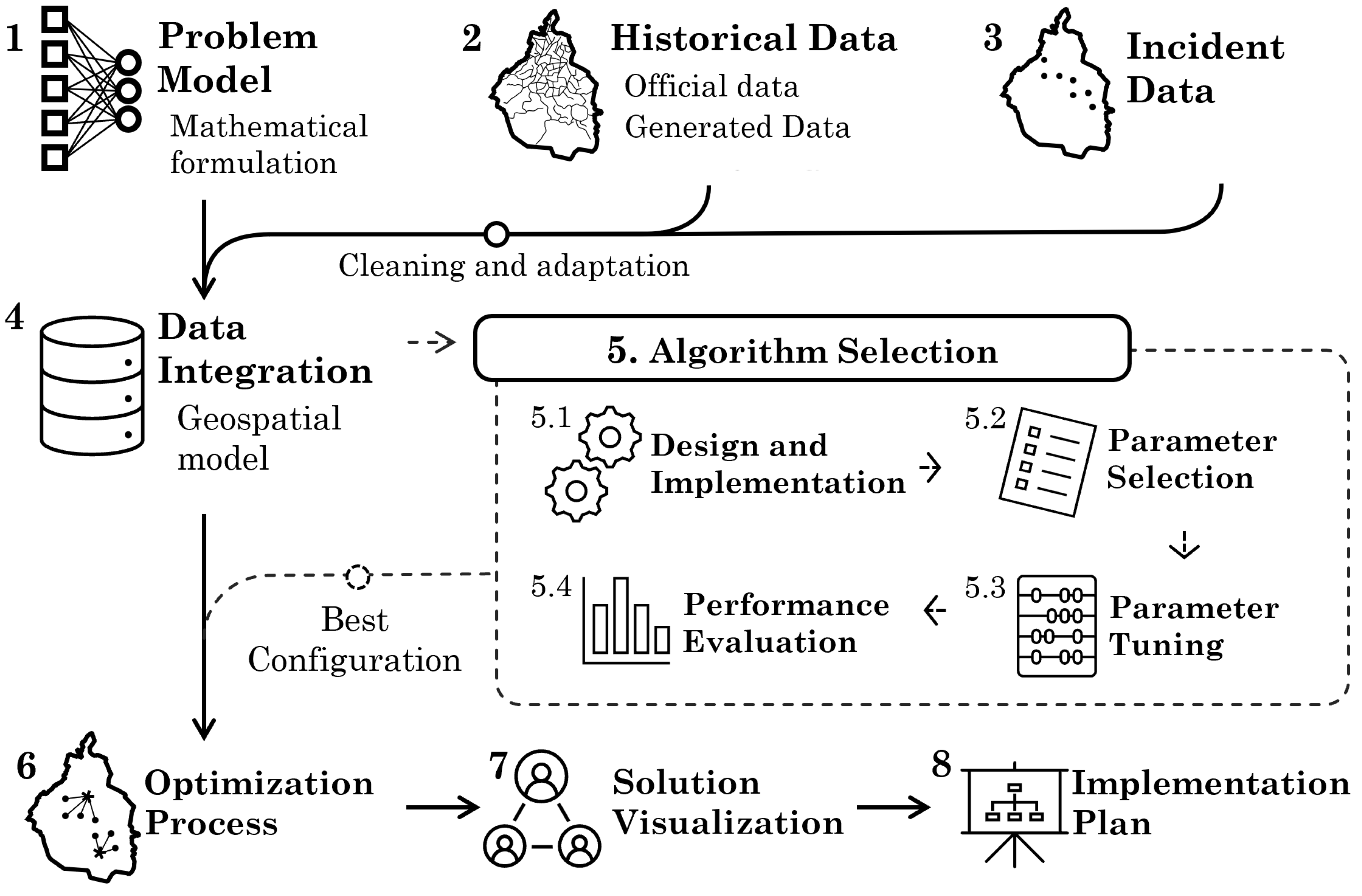
The proposed methodology is shown in
Figure 1 and consists of eight stages: Problem Model, Historical Data, Incident Data, Data Integration, Algorithm Selection, Optimization Process, Solution Visualization, and Implementation Plan. The purpose of each stage and its components are described in the following.
3.3. Incident Data
In this stage, event information is collected from the location of the demand points, considering the confirmed or possible number of victims, as well as blocked roads, traffic data, and available hospital capacity. In a real scenario, these data are obtained from government sources as the information is being integrated. In an experimental scenario, historical data from previous incidents are used.
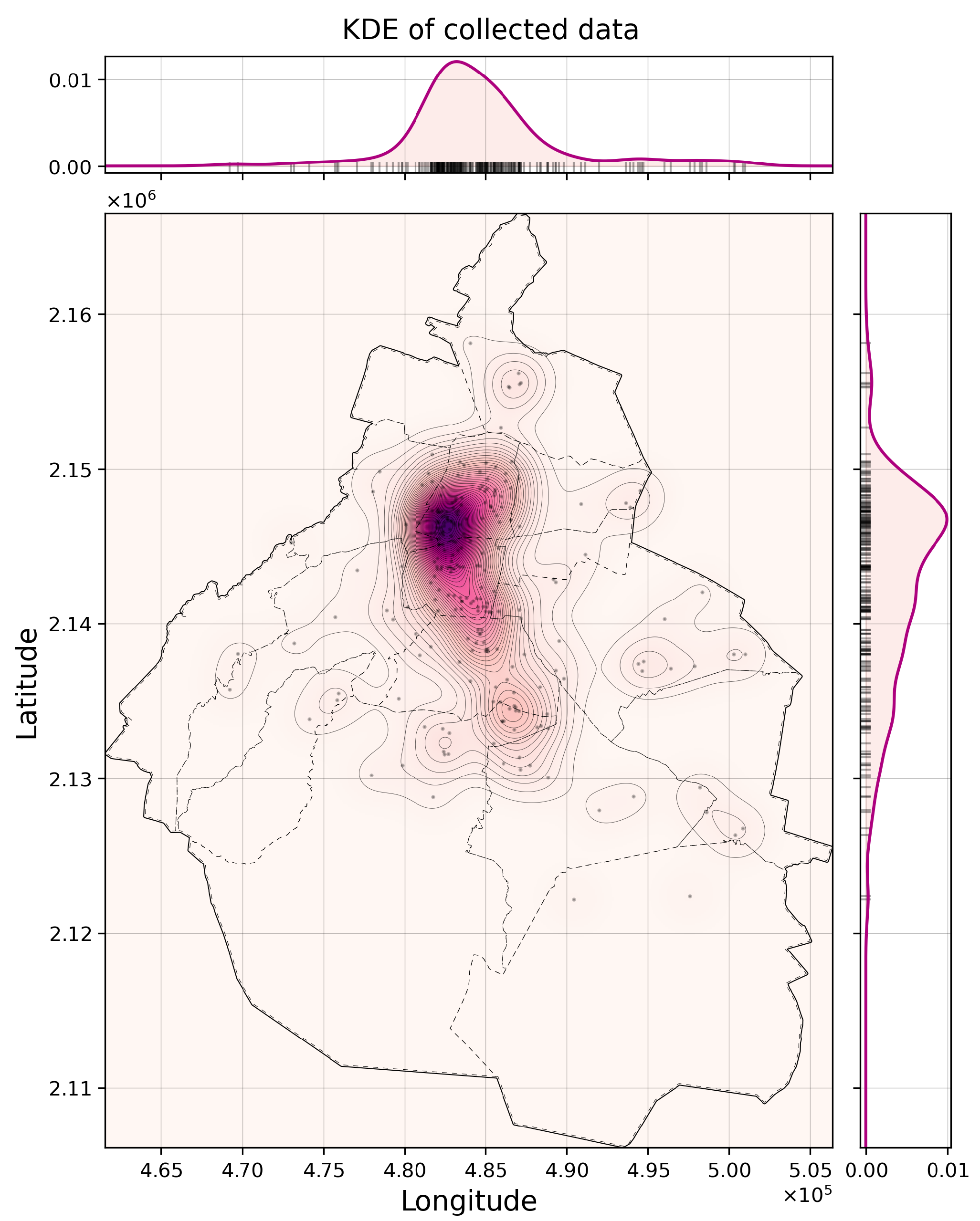
Location of demand points. The CDMX Open Data Portal provides georeferenced data on buildings that collapsed or suffered damage during the 19 September 2017 earthquake, which can be used to estimate the probability distribution of damage locations that could occur in future events. It is proposed to generate new hypothetical scenarios that follow this spatial distribution and enable an adjustment of the algorithm parameters based on different instances of the same problem, using the kernel density estimation of the buildings damaged in the 2017 earthquake, and using the library scikit learn and a Gaussian kernel. To determine the bandwidth of the kernel, a grid search is performed (in one dimension) with 1000 values of powers of 10, from to . For each bandwidth value, the KDE is obtained using the leave one out validation method, and selecting the maximum likelihood logarithmic estimation.
In addition, the demand for each of them has to be estimated. In a real scenario, the responsible official reports the location of the incident and its characteristics to make an initial estimation of the damage per quadrant [
40]. This estimation includes details of damaged buildings (does not change), as well as the number of victims (may change as more specific information becomes available). The official data reported in the September 2017 earthquake do not have this information; therefore, it is proposed to make an approximation of the number of victims by using the points generated with the kernel density, the data from the land census, and the SEDUVI, which requires the following modifications:
Only residential buildings with information on the number of levels are considered.
If a building does not have the number of levels but the height, then half of the height in meters is used as the number of levels.
For blocks that do not have the average number of occupants, the average of the surrounding blocks is used.
To estimate the number of victims in each , the following steps were performed:
n points are sampled using the kernel with ;
Search for the nearest building in the land records layer using Euclidean distance.
The block in which each building is located is identified by calculating the Euclidean distance between the building and the centroids of the blocks.
The average number of occupants per apartment in the block is taken and rounded to the closest integer using the ceiling function.
If the building has three floors or less, it is considered a single-family unit, so the number of victims of the block is equal to .
If the building has more than three levels, it is considered a multi-family building, and the average number of residents in the block is multiplied by the number of levels .
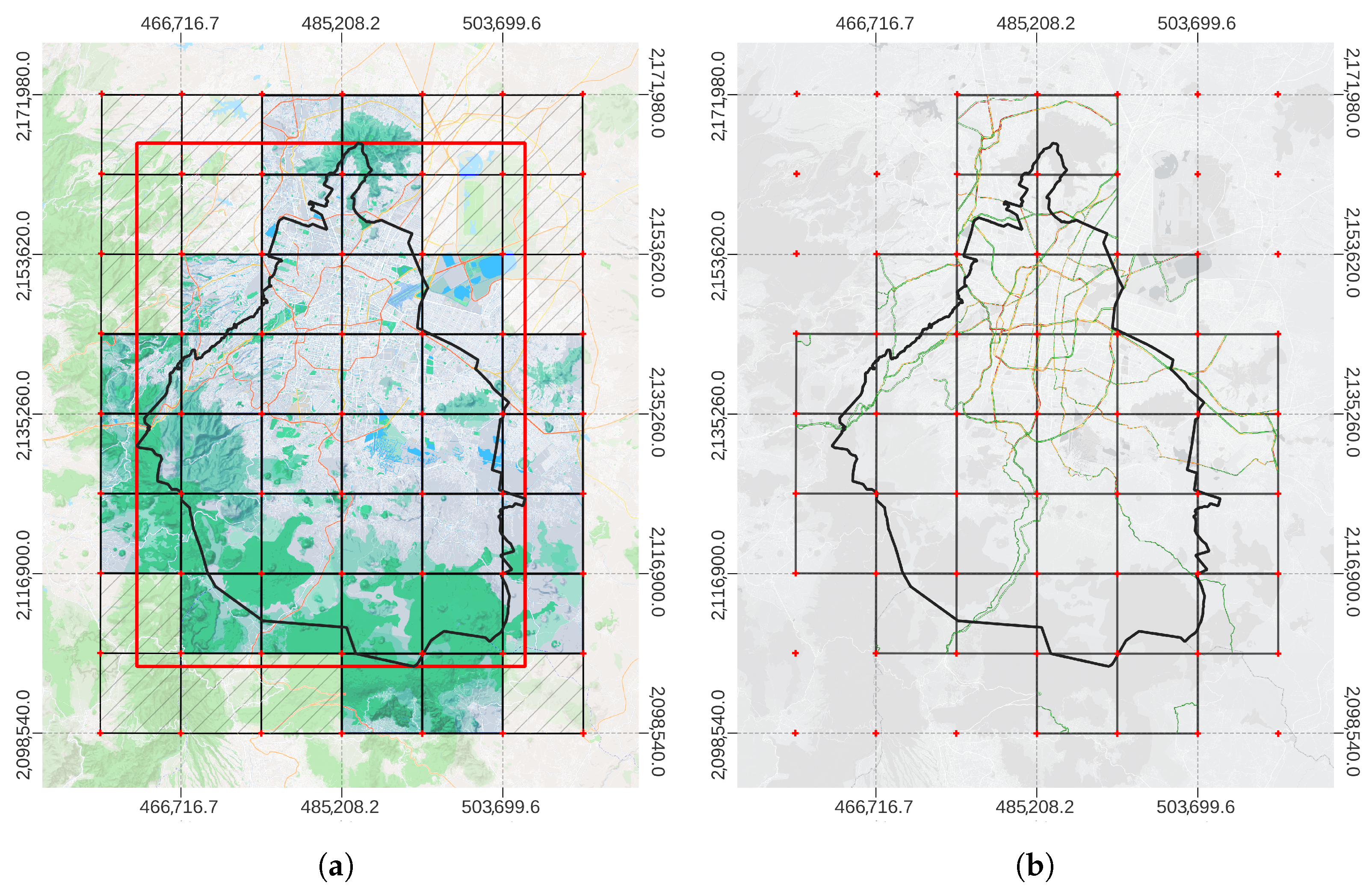
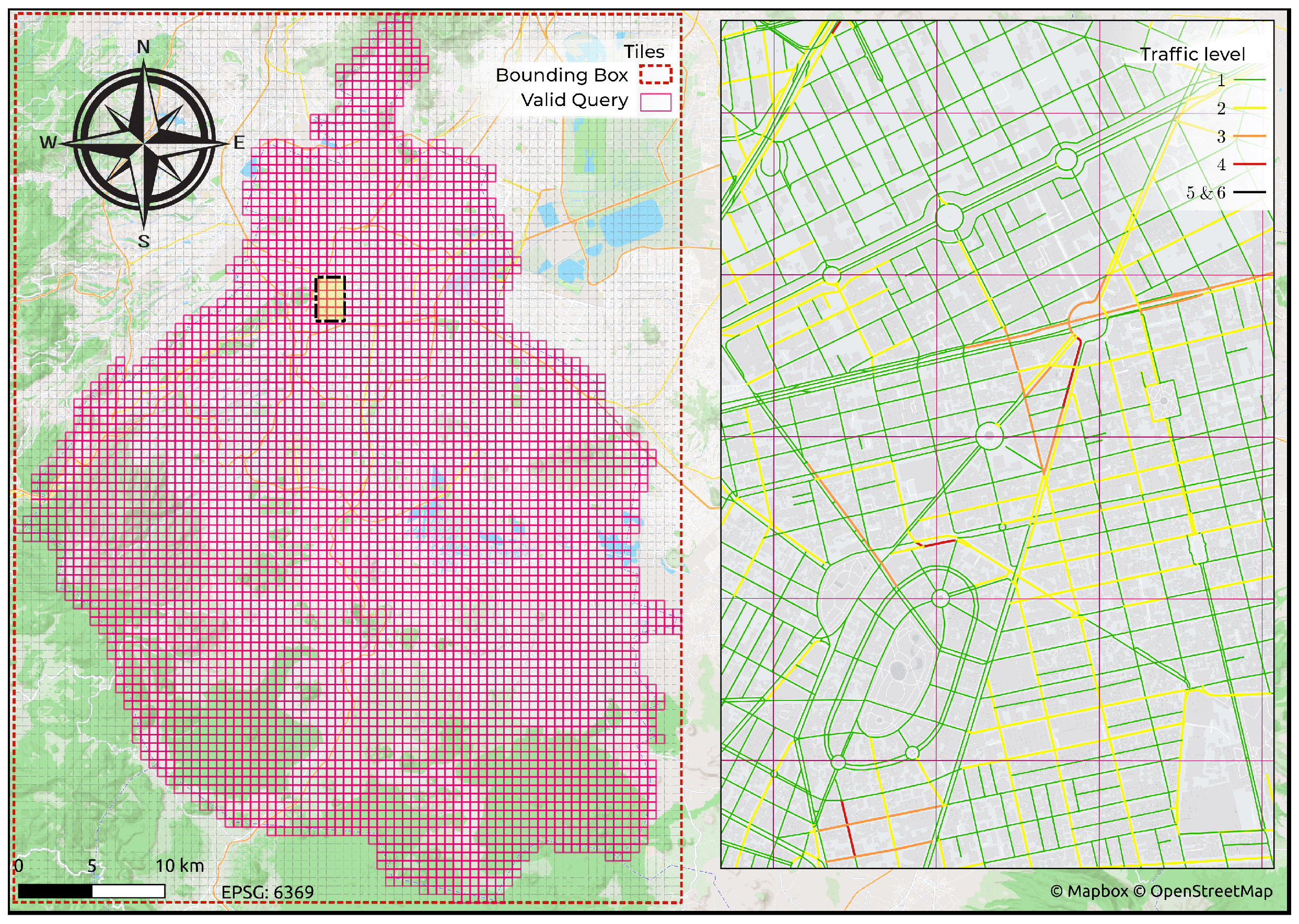
Traffic data. Traffic data can be obtained in real time through TomTom’s TrafficFlow API according to the specifications provided on the website, which is in raster format and segmented into fixed-size rectangular tiles, representing an exponential division of space [
41], as is described in
Figure 5a. To optimize the memory required to maintain all tiles, the data are converted to single-band rasters that preserve the different traffic classes by mapping the RGB components with a range of
to a class index of
; see
Figure 5b.
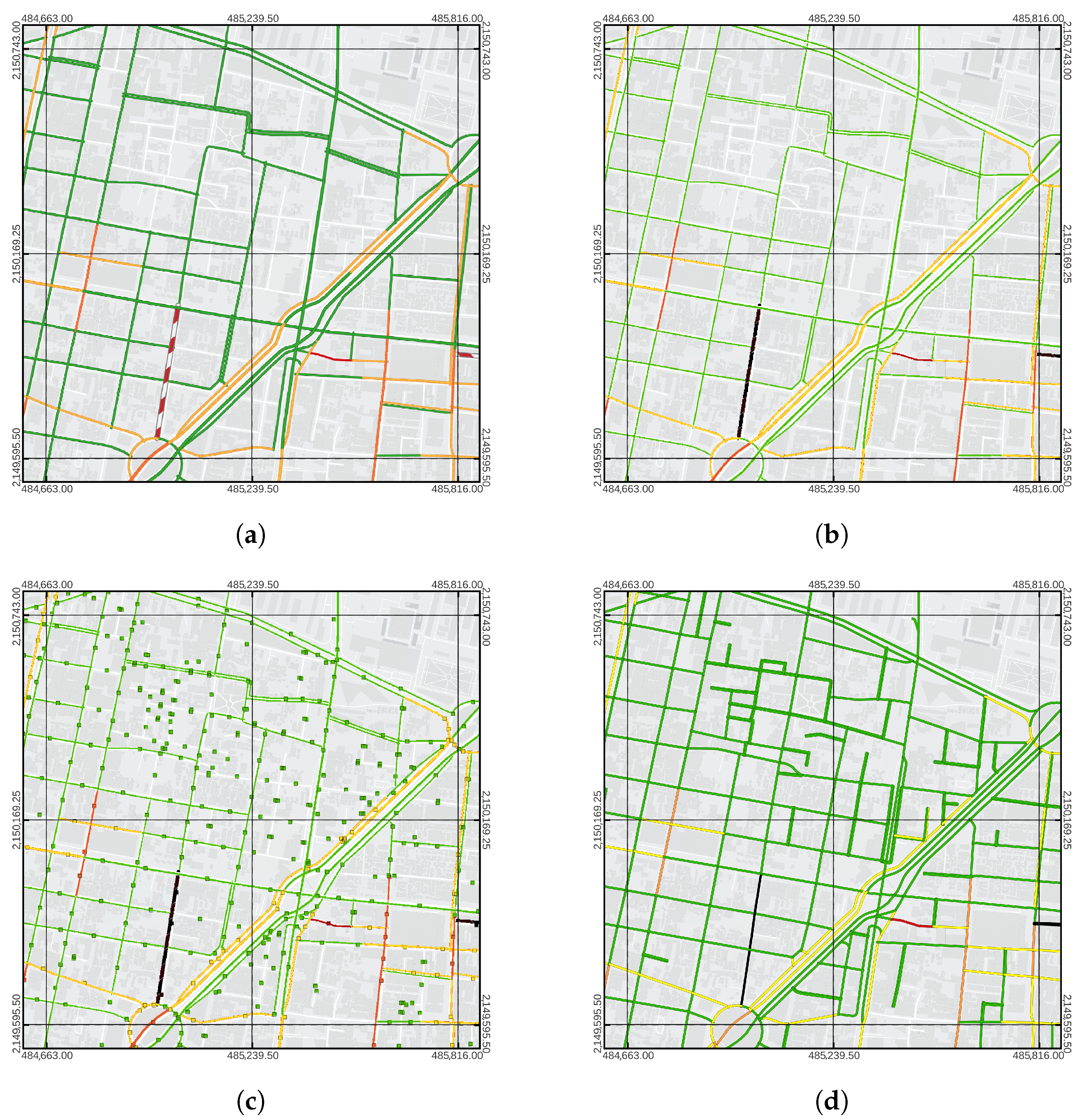
When tiles are available as single-band raster data, a sampling is performed for each edge of the graph. This is performed by calculating the center of the sampling window, which is the end of the line segment perpendicular to the intermediate line segment of the edge geometry and crossing its center. The final result of the extraction of traffic data is a Pandas dataframe that associates the id of each edge with an integer value for each color that corresponds to the most commonly used value in the sampling window. However, if the sample window does not contain a number other than 0, it is assumed to represent free traffic segment and the number 1 is assigned.
5. Conclusions and Future Work
Relevant data can be obtained from official data sources in the study area to solve the location-allocation problem of ambulances in Mass Casualty Incidents with multiple demand points, integrating historical data of disaster incidents; the location of complementary resources, such as hospitals, temporary shelters, and collection centers; and the geographical delimitation of regions of care designated by the authorities of emergency services.
The proposed methodology to determine candidate emergency response areas (candidate bases) allows us to find a subset of 1846 representative vertices on the graph that model the road transport network, from which at least of the remaining vertices are expected to reach within 9 min at 40 km/h, considering different daytime values. In contrast to the alternative of using the complete road transport network in the problem model, the resulting search space contains only of the original graph. Although the identification of candidate bases is performed statically, it is possible to discard more bases considering complementary event data, such as traffic data.
By obtaining the set of roads that can be used as temporary ambulance bases with their respective capacities, the location of the demand points with their respective estimated number of victims, and the graph that models the road transport network, it is possible to analyze the location-allocation problem as a multi-objective optimization problem. This model requires the identification of the candidate bases to be activated (location) and the demand point served by each one (allocation), subject to eight constraints that ensure the congruence of the solution and limit the solutions to viable regions, considering the maximum response time or the maximum number of candidate bases to be activated.
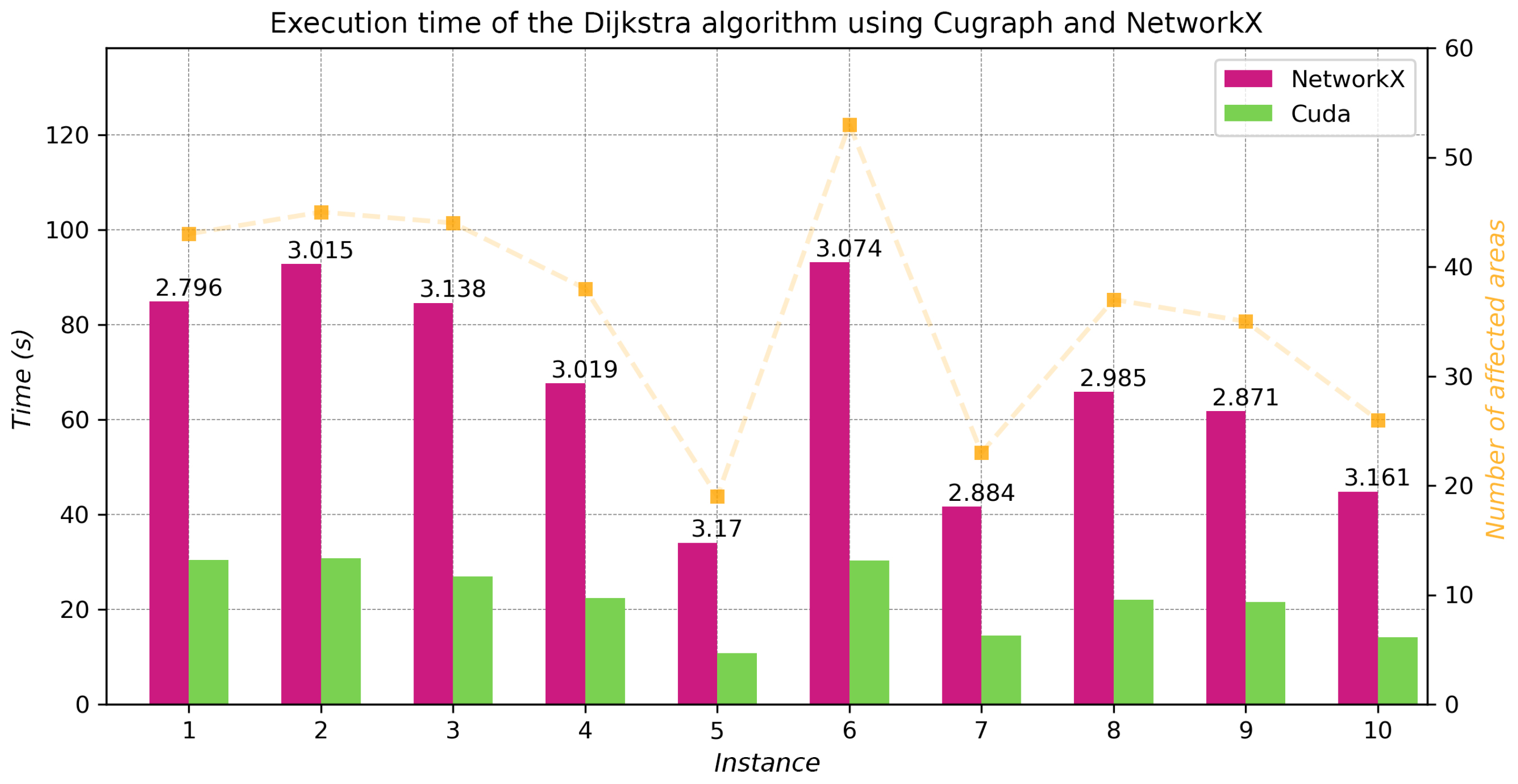
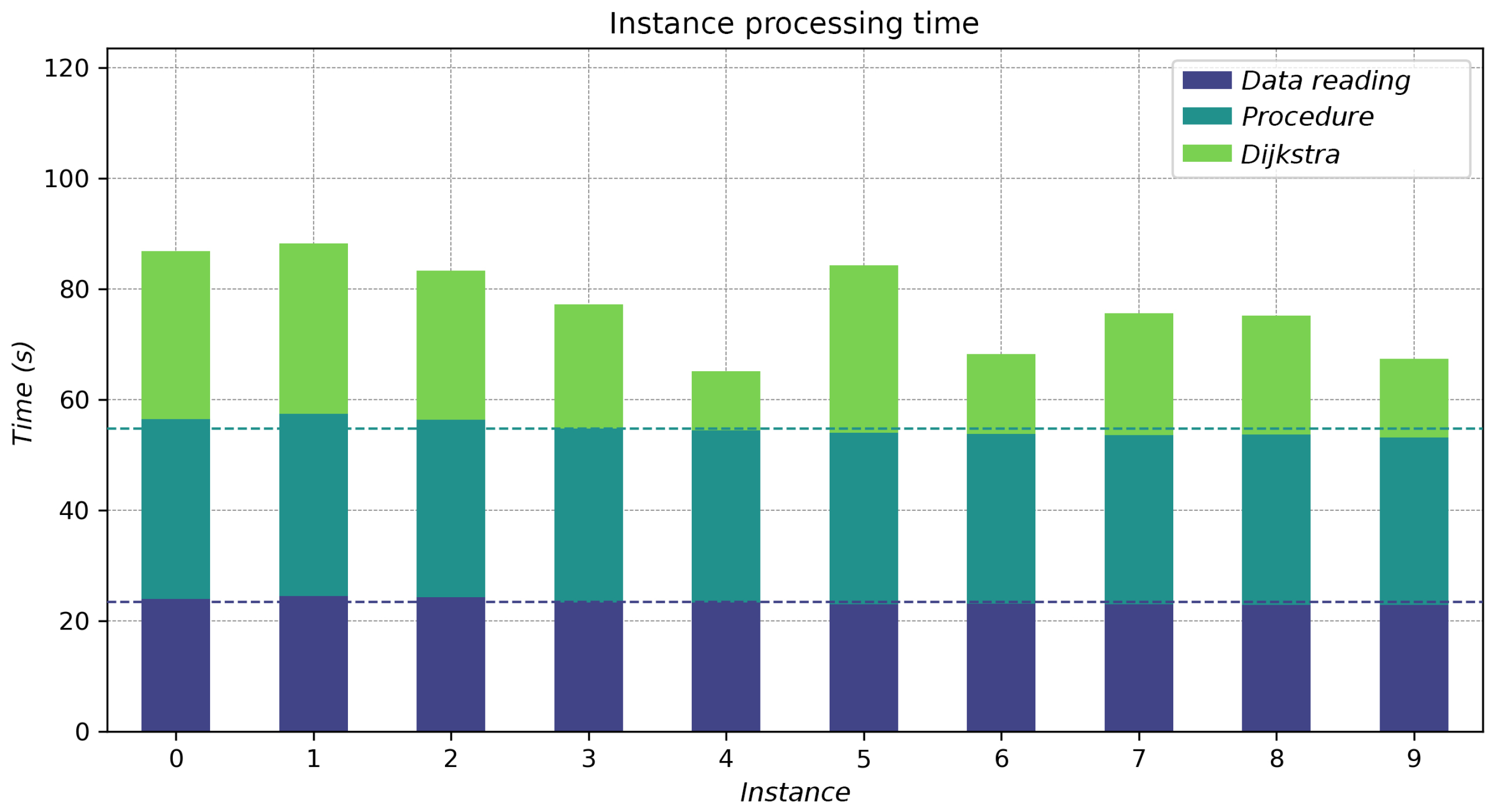
By using the Kernel Density Estimation of the historical data of buildings damaged by the 19 September 2017 earthquake, it is possible to generate hypothetical scenarios of the problem. For each scenario (hypothetical or real), a specific instance of the same problem was generated. To generate such an instance, the read time of the data and the procedure have approximately the same duration, but the time needed to compute the cost matrix is proportional to the number of demand points. The Dijkstra algorithm was used to obtain the cost matrix by inverting the graph and running it twice for each demand point, using as the origin the end points of the edge that is closest to the demand points. Implementing this algorithm using graphs from the cuGraph library accelerated this calculation by approximately compared to the implementation of the NetworkX library. The NSGA-II algorithm, implemented with the proposed parameters, allows us to find solutions that adapt to the two objectives considered and to the multiple constraints established. The elite configurations found in the parameter tuning stage for the NSGA-II algorithm have a better evaluation with the hypervolume indicator and have a tendency to converge on Pareto fronts that are close to the best known optimal zone compared to other regular configurations. The obtained parameters of the elite configurations suggest that it is preferable to have large population sizes (200 individuals), to use the urgency-based allocation method, to perform mutation repair, and to have a small initialization probability (0.1–0.25). Regarding time-interrupted configurations, it can be observed that increasing the percentage of descendants significantly increases execution time, so it is preferable to keep it in the middle (0.5) to avoid bottlenecks. However, the best option to compare these configurations would be to implement the time-based termination criterion instead of aborting when the execution time is exceeded. The urgency-based allocation method was considered one of the best configurations compared to the classic and the demand–urgency-based methods, suggesting that the relationship between base capacity and urgency at the demand point in this problem is not significant enough to benefit from a method that considers demand first and urgency afterward.
The possible parameter values included populations of small size (20, 50) and a percentage of descendants. On the other hand, the mutation repair method outperformed the normal repair method, indicating that the procedure used to discard already explored solutions tends to improve the performance of the algorithm. A more rigorous analysis is needed to verify the relationship between these parameters and the algorithm performance, but these results provide a baseline for designing the required experiments.
The evaluation of the elite configurations on three representative instances with 20 random seeds suggests that although these configurations stand out from other regular configurations evaluated in parameter tuning, better techniques and configurations still need to be evaluated to obtain more accurate results with less variability, exploring solutions on the Pareto front with a smaller number of activated bases. However, the quality of the solutions is improved by merging the Pareto fronts of multiple runs of the same configuration, with the disadvantage of requiring more time. Furthermore, by parallelizing the multiple runs to generate the unified Pareto front, the result was obtained in half the time of a sequential execution.
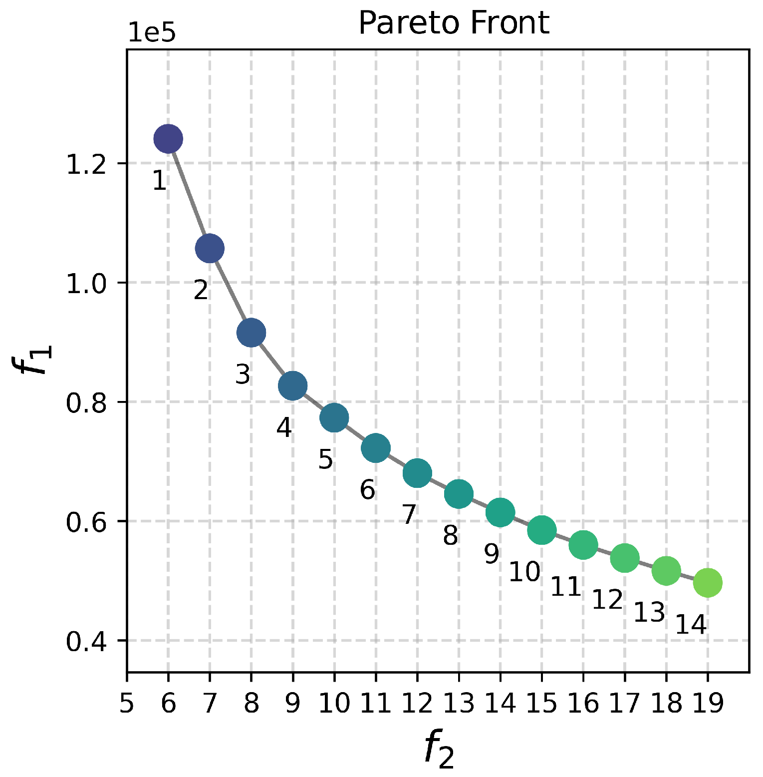
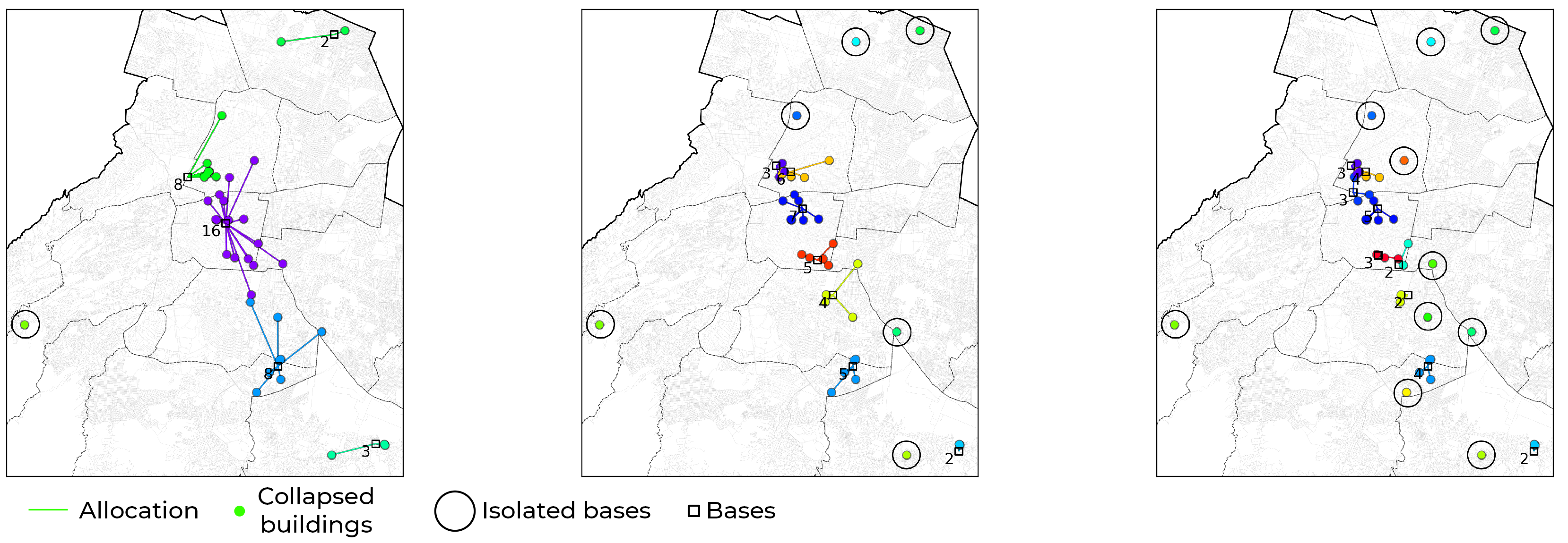
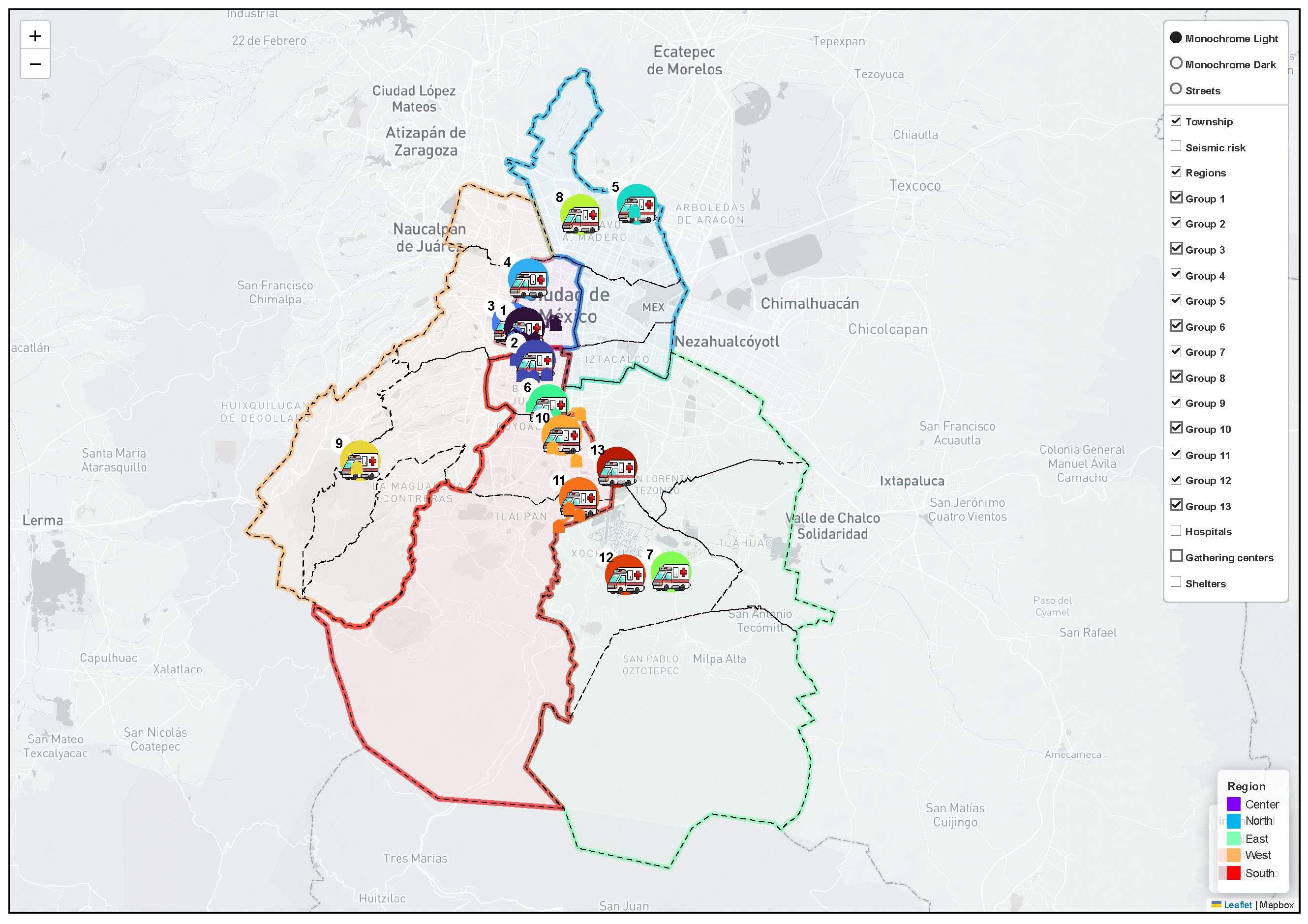
The different solutions of the Pareto front suggest different ways of assigning the ambulances to the focus locations, and the pre-visualizations allow for the intuitive identification of which points remain isolated and which bases should be activated. The final visualization, generated in HTML format, can be used for further implementation in a context that allows the emergency medical services involved in the care plan to visualize the information interactively, to show or hide elements of interest depending on the circumstances.
The comparison of the results with other algorithms is important in future work. However, in this paper, the main objective focuses on the mathematical modeling of the problem and the integration of real data that could be obtained during a large-scale emergency scenario, from which the quality of solutions can be described. Thus, this work represents a useful starting point for future studies.
Author Contributions
Conceptualization, M.S.-P. and G.G.; methodology, M.M.-P. and M.S.-P.; software, V.K.L.-S. and G.G.; validation, G.G. and M.S.-P.; formal analysis, M.M.-P. and V.K.L.-S.; investigation, M.M.-P. and V.K.L.-S.; resources, V.K.L.-S. and M.S.-P.; data curation, G.G. and M.M.-P.; writing—original draft preparation, V.K.L.-S. and M.M.-P.; writing—review and editing, G.G. and M.M.-P.; visualization, M.M.-P. and V.K.L.-S.; supervision, G.G. and M.M.-P.; project administration, M.S.-P. and G.G.; funding acquisition, M.S.-P. and G.G. All authors have read and agreed to the published version of the manuscript.
Funding
This work was partially sponsored by the Instituto Politécnico Nacional under grants 20240426, 20240632, and by the Consejo Nacional de Humanidades, Ciencias y Tecnologías (CONAHCYT) under grants 960525 and 1183927.
Institutional Review Board Statement
Not applicable.
Informed Consent Statement
Not applicable.
Data Availability Statement
Acknowledgments
We are thankful to the reviewers for their time and invaluable and constructive feedback, which helped improve the quality of the paper.
Conflicts of Interest
The authors declare no conflicts of interest.
References
- The International Federation of Red Cross and Red Crescent Societies. What Is a Disaster? Available online: https://www.ifrc.org/what-disaster (accessed on 4 November 2022).
- World Health Organization. Emergency Cycle. Available online: https://www.who.int/europe/emergencies/emergency-cycle (accessed on 4 November 2022).
- American college of surgeons committee on trauma and Campos, Víctor and Roig, Félix Garcia. In PHTLS Soporte Vital de Trauma Preshospitalario; Jones & Bartlett Learning: Burlington, MA, USA, 2020.
- International Resources Group and “Oficina de los Estados Unidos de Asistencia para Desastres en el Extranjero para Latino América y el Caribe”. Curso Básico Sistema de Comando de Incidentes. 2021. Available online: https://www.gob.mx/cms/uploads/attachment/file/228836/Curso_Basico_SCI_material_de_referencia.pdf (accessed on 14 September 2022).
- Halper, R.; Raghavan, S.; Sahin, M. Local search heuristics for the mobile facility location problem. Comput. Oper. Res. 2015, 62, 210–223. [Google Scholar] [CrossRef]
- Barojas-Payán, E.; Sánchez-Partida, D.; Gibaja-Romero, D.E.; Martínez-Flores, J.L.; Cabrera-Rios, M. Optimization Model to Locate Pre-positioned Warehouses and Establish Humanitarian Aid Inventory Levels. In Disaster Risk Reduction in Mexico: Methodologies, Case Studies, and Prospective Views; Springer International Publishing: Cham, Switzerland, 2021; pp. 169–192. [Google Scholar] [CrossRef]
- Zaffar, M.A.; Rajagopalan, H.K.; Saydam, C.; Mayorga, M.; Sharer, E. Coverage, survivability or response time: A comparative study of performance statistics used in ambulance location models via simulation–optimization. Oper. Res. Health Care 2016, 11, 1–12. [Google Scholar] [CrossRef]
- Mohri, S.S.; Haghshenas, H. An ambulance location problem for covering inherently rare and random road crashes. Comput. Ind. Eng. 2021, 151, 106937. [Google Scholar] [CrossRef]
- Toregas, C.; Swain, R.; ReVelle, C.; Bergman, L. The Location of Emergency Service Facilities. Oper. Res. 1971, 19, 1363–1373. [Google Scholar] [CrossRef]
- Kaveh, M.; Mesgari, M.S. Improved biogeography-based optimization using migration process adjustment: An approach for location-allocation of ambulances. Comput. Ind. Eng. 2019, 135, 800–813. [Google Scholar] [CrossRef]
- Hashtarkhani, S.; Matthews, S.A.; Yin, P.; Mohammadi, A.; Mohammad Ebrahimi, S.; Tara, M.; Kiani, B. Where to place emergency ambulance vehicles: Use of a capacitated maximum covering location model with real call data. Geospat. Health 2023, 18, 1198. [Google Scholar] [CrossRef]
- Barojas-Payán, E.; Sánchez-Partida, D.; Caballero-Morales, S.O.; Martínez-Flores, J.L. A Hybrid Capacitated Multi-facility Location Model for Pre-positioning Warehouses and Inventories in Regions at Risk in Mexico. In Disaster Risk Reduction in Mexico: Methodologies, Case Studies, and Prospective Views; Springer International Publishing: Cham, Switzerland, 2021; pp. 193–221. [Google Scholar] [CrossRef]
- Zheng, Y.J.; Chen, S.Y.; Ling, H.F. Evolutionary optimization for disaster relief operations: A survey. Appl. Soft Comput. 2015, 27, 553–566. [Google Scholar] [CrossRef]
- Deb, K.; Pratap, A.; Agarwal, S.; Meyarivan, T. A fast and elitist multiobjective genetic algorithm: NSGA-II. IEEE Trans. Evol. Comput. 2002, 6, 182–197. [Google Scholar] [CrossRef]
- Nolz, P.C.; Doerner, K.F.; Gutjahr, W.J.; Hartl, R.F. A Bi-objective Metaheuristic for Disaster Relief Operation Planning. In Advances in Multi-Objective Nature Inspired Computing; Coello Coello, C.A., Dhaenens, C., Jourdan, L., Eds.; Springer: Berlin/Heidelberg, Germany, 2010; pp. 167–187. [Google Scholar] [CrossRef]
- Chang, F.S.; Wu, J.S.; Lee, C.N.; Shen, H.C. Greedy-search-based multi-objective genetic algorithm for emergency logistics scheduling. Expert Syst. Appl. 2014, 41, 2947–2956. [Google Scholar] [CrossRef]
- Schjølberg, M.E.; Bekkevold, N.P.; Sánchez-Díaz, X.; Mengshoel, O.J. Comparing Metaheuristic Optimization Algorithms for Ambulance Allocation: An Experimental Simulation Study. In Proceedings of the Genetic and Evolutionary Computation Conference, GECCO ’23, Lisbon, Portugal, 15–19 July 2023; pp. 1454–1463. [Google Scholar] [CrossRef]
- Saeidian, B.; Mesgari, M.S.; Ghodousi, M. Evaluation and comparison of Genetic Algorithm and Bees Algorithm for location–allocation of earthquake relief centers. Int. J. Disaster Risk Reduct. 2016, 15, 94–107. [Google Scholar] [CrossRef]
- Geng, J.; Hou, H.; Geng, S. Optimization of Warehouse Location and Supplies Allocation for Emergency Rescue under Joint Government–Enterprise Cooperation Considering Disaster Victims’ Distress Perception. Sustainability 2021, 13, 10560. [Google Scholar] [CrossRef]
- Alinaghian, M.; Hejazi, S.R.; Bajoul, N.; Sadeghi Velni, K. A novel robust model for location-allocation of healthcare facilities considering pre-disaster and post-disaster characteristics. Sci. Iran. 2023, 30, 619–641. [Google Scholar] [CrossRef]
- Oksuz, M.K.; Satoglu, S.I. Integrated optimization of facility location, casualty allocation and medical staff planning for post-disaster emergency response. J. Humanit. Logist. Supply Chain. Manag. 2023; ahead-of-print. [Google Scholar] [CrossRef]
- Qi, W.; Ovur, S.E.; Li, Z.; Marzullo, A.; Song, R. Multi-Sensor Guided Hand Gesture Recognition for a Teleoperated Robot Using a Recurrent Neural Network. IEEE Robot. Autom. Lett. 2021, 6, 6039–6045. [Google Scholar] [CrossRef]
- Zhao, J.; Lv, Y.; Zeng, Q.; Wan, L. Online Policy Learning-Based Output-Feedback Optimal Control of Continuous-Time Systems. IEEE Trans. Circuits Syst. II Express Briefs 2024, 71, 652–656. [Google Scholar] [CrossRef]
- Medina-Perez, M.; Legaria-Santiago, V.K.; Guzmán, G.; Saldana-Perez, M. Search Space Reduction in Road Networks for the Ambulance Location and Allocation Optimization Problems: A Real Case Study. In Telematics and Computing; Mata-Rivera, M.F., Zagal-Flores, R., Barria-Huidobro, C., Eds.; Springer: Cham, Switzerland, 2023; pp. 157–175. [Google Scholar]
- Karpova, Y.; Villa, F.; Vallada, E.; Ángel Vecina, M. Heuristic algorithms based on the isochron analysis for dynamic relocation of medical emergency vehicles. Expert Syst. Appl. 2023, 212, 118773. [Google Scholar] [CrossRef]
- Caglayan, N.; Satoglu, S.I. Multi-Objective Two-Stage Stochastic Programming Model for a Proposed Casualty Transportation System in Large-Scale Disasters: A Case Study. Mathematics 2021, 9, 316. [Google Scholar] [CrossRef]
- Wang, J.; Wang, Y.; Yu, M. A multi-period ambulance location and allocation problem in the disaster. J. Comb. Optim. 2020, 43, 909–932. [Google Scholar] [CrossRef]
- Nadar, R.A.; Jha, J.; Thakkar, J.J. Adaptive variable neighbourhood search approach for time-dependent joint location and dispatching problem in a multi-tier ambulance system. Comput. Oper. Res. 2023, 159, 106355. [Google Scholar] [CrossRef]
- Daskin, M.S.; Maass, K.L. The p-Median Problem. In Location Science; Springer International Publishing: Cham, Switzerland, 2015; pp. 21–45. [Google Scholar] [CrossRef]
- Ghoseiri, K.; Ghannadpour, S.F. Solving capacitated p-median problem using genetic algorithm. In Proceedings of the 2007 IEEE International Conference on Industrial Engineering and Engineering Management, Singapore, 2–4 December 2007. [Google Scholar] [CrossRef]
- Instituto Nacional de Estadística y Geografía (INEGI). Límite de Alcaldías (áreas Geoestadísticas Municipales). 2023. Available online: https://datos.cdmx.gob.mx/dataset/alcaldias (accessed on 1 August 2023).
- Secretaría de Gestión Integral de Riesgos y Protección Civil (SGIRPC). Capas Relacionadas al Sismo del 19/09/2017: Inmuebles Colapsados, Zona de Mayor Afectación e Infraestructura Dañada, Zonas de Riesgo Sísmico. Available online: https://www.atlas.cdmx.gob.mx/datosabiertos2.html (accessed on 1 August 2023).
- Órgano de Difusión del Gobierno de la Ciudad de México. Gaceta Oficial de la Ciudad de México, No. 685 Bis. Protocolo del Plan de Emergencia Sísmica. 2021. Available online: https://data.consejeria.cdmx.gob.mx/portal_old/uploads/gacetas/18652b057da05daee4cf7a0784093fff.pdf (accessed on 26 March 2023).
- Instituto de Planeación Democrática y Prospectiva. Hospitales Públicos y Privados en Operación de la ZMVM. 2023. Available online: https://datos.cdmx.gob.mx/dataset/hospitales-publicos-y-privados-en-operacion-de-la-zmvm (accessed on 1 August 2023).
- Secretaría de Gestión Integral de Riesgos y Protección Civil. 22 Conjuntos de Datos de Secretaría de Gestión Integral de Riesgos y Protección Civil. 2023. Available online: https://datos.cdmx.gob.mx/organization/secretaria-de-gestion-integral-de-riesgos-y-proteccion-civil (accessed on 1 August 2023).
- Secretaría de Gestión Integral de Riesgos y Protección Civil. Refugios Temporales. 2023. Available online: https://datos.cdmx.gob.mx/dataset/refugios (accessed on 1 August 2023).
- Instituto Nacional de Estadística y Geografía (INEGI). Polígonos de Manzanas de la Ciudad de México. 2023. Available online: https://datos.cdmx.gob.mx/dataset/poligonos-de-manzanas-de-la-ciudad-de-mexico (accessed on 1 August 2023).
- Secretaría de Desarrollo Urbano y Vivienda (SEDUVI). Descarga de Datos SEDUVI. 2023. Available online: https://sig.cdmx.gob.mx/datos/descarga#d_datos_seduvi (accessed on 1 September 2023).
- Secretaría de Administración y Finanzas (SAF). Descarga de Datos del Catastro. 2023. Available online: https://sig.cdmx.gob.mx/datos/descarga#d_datos_cat (accessed on 1 September 2023).
- Secretaria de Gestión Integral de Riesgos y Protección Civil de la Ciudad de México and Urzúa, Myriam. Protocolo del Plan de Emergencia Sísmica; Gaceta oficial de la Ciudad de México: Mexico City, Mexico, 2021. [Google Scholar]
- TomTom Developers. Zoom Levels and Tile Grid. 2023. Available online: https://developer.tomtom.com/map-display-api/documentation/zoom-levels-and-tile-grid (accessed on 9 September 2023).
- Liang, J.J.; Yue, C.T.; Qu, B.Y. Multimodal multi-objective optimization: A preliminary study. In Proceedings of the 2016 IEEE Congress on Evolutionary Computation (CEC), Vancouver, BC, Canada, 24–29 July 2016; pp. 2454–2461. [Google Scholar] [CrossRef]
- Ma, H.; Zhang, Y.; Sun, S.; Liu, T.; Shan, Y. A comprehensive survey on NSGA-II for multi-objective optimization and applications. Artif. Intell. Rev. 2023, 56, 15217–15270. [Google Scholar] [CrossRef]
- Ahmadi, M.H.; Ahmadi, M.A. Multi objective optimization of performance of three-heat-source irreversible refrigerators based algorithm NSGAII. Renew. Sustain. Energy Rev. 2016, 60, 784–794. [Google Scholar] [CrossRef]
- Pymoo: Multi-Objective Optimization in Python. Available online: https://www.pymoo.org (accessed on 2 September 2023).
- López-Ibáñez, M.; Dubois-Lacoste, J.; Pérez Cáceres, L.; Birattari, M.; Stützle, T. The Irace Package: User Guide. 2022. Available online: https://cran.r-project.org/web/packages/irace/vignettes/irace-package.pdf (accessed on 21 October 2023).
- Fitch, J. Response times: Myths, measurement & management. JEMS J. Emerg. Med Serv. 2005, 30, 46–56. [Google Scholar] [CrossRef]
- Wu, C.; Hwang, K.P. Using a Discrete-event Simulation to Balance Ambulance Availability and Demand in Static Deployment Systems. Acad. Emerg. Med. 2009, 16, 1359–1366. [Google Scholar] [CrossRef] [PubMed]
- Tian, Z.; Zhang, Z.; Ning, C.; Peng, T.; Guo, Y.; Cao, Z. Multi-objective optimization of cable force of arch bridge constructed by cable-stayed cantilever cast-in-situ method based on improved NSGA-II. Structures 2024, 59, 105782. [Google Scholar] [CrossRef]
- Bora, T.C.; Mariani, V.C.; dos Santos Coelho, L. Multi-objective optimization of the environmental-economic dispatch with reinforcement learning based on non-dominated sorting genetic algorithm. Appl. Therm. Eng. 2019, 146, 688–700. [Google Scholar] [CrossRef]
- de Souza, M.; Ritt, M.; López-Ibáñez, M.; Cáceres, L.P. ACVIZ: A Tool for the Visual Analysis of the Configuration of Algorithms with irace. Oper. Res. Perspect. 2021, 8, 100–186. [Google Scholar] [CrossRef]
Figure 1.
Proposed methodology.
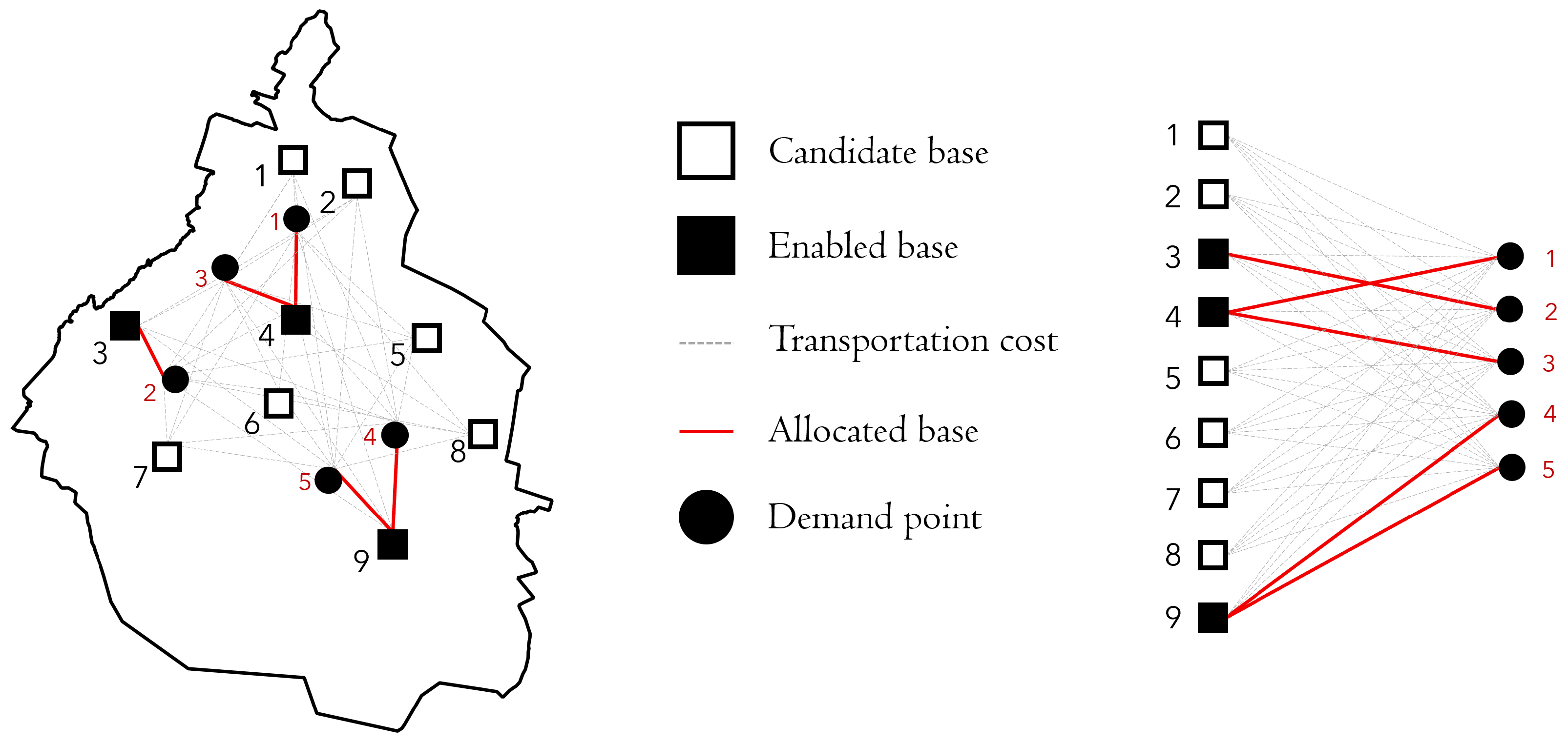
Figure 2.
Representation of the problem using a bipartite graph.
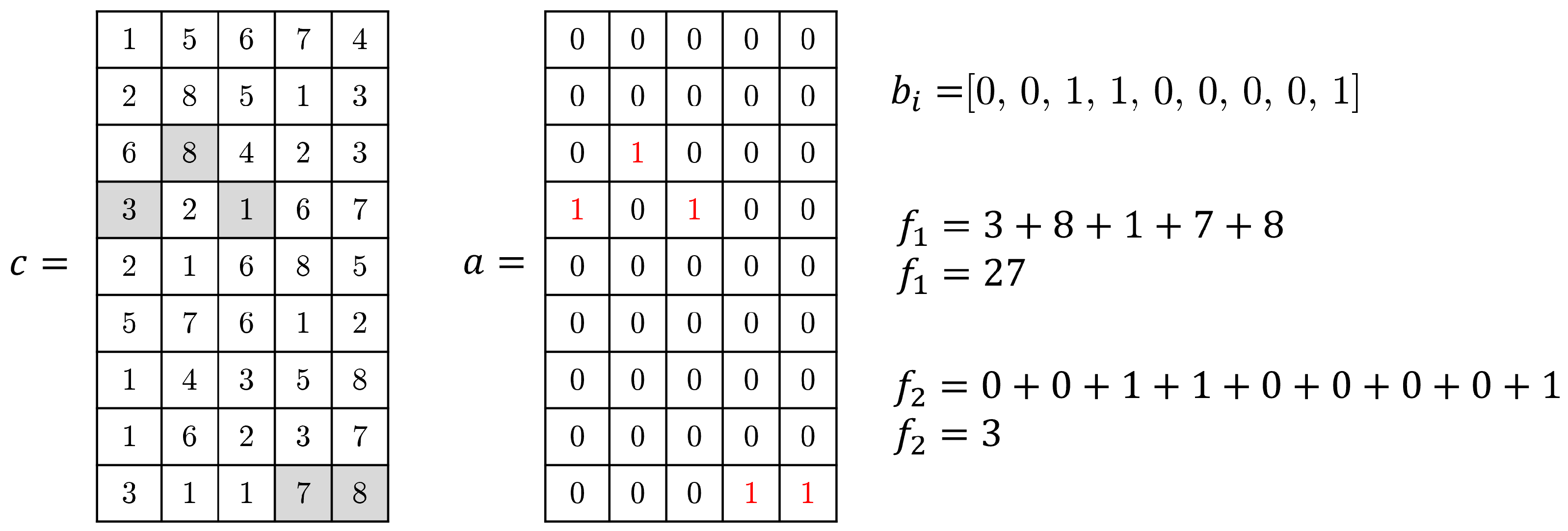
Figure 3.
Decision variables and fitness value of the solution for the scenario represented in
Figure 2.
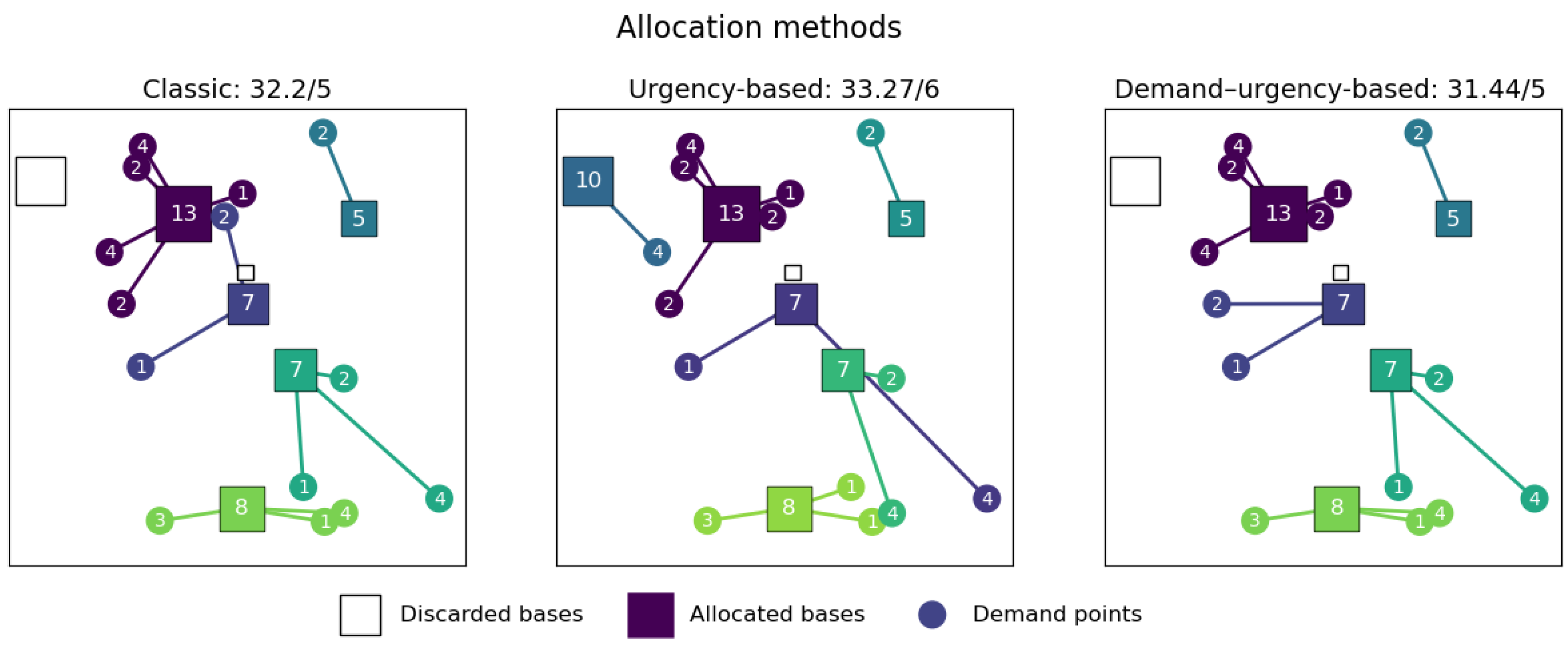
Figure 4.
Example of allocation methods.
Figure 5.
Mexico City traffic on 20 October 2023 at 18:58 obtained with a zoom level of 12. (a) Tiles required to cover the bounding box in Mexico City (red box). (b) Final result of conversion to single-band raster.
Figure 6.
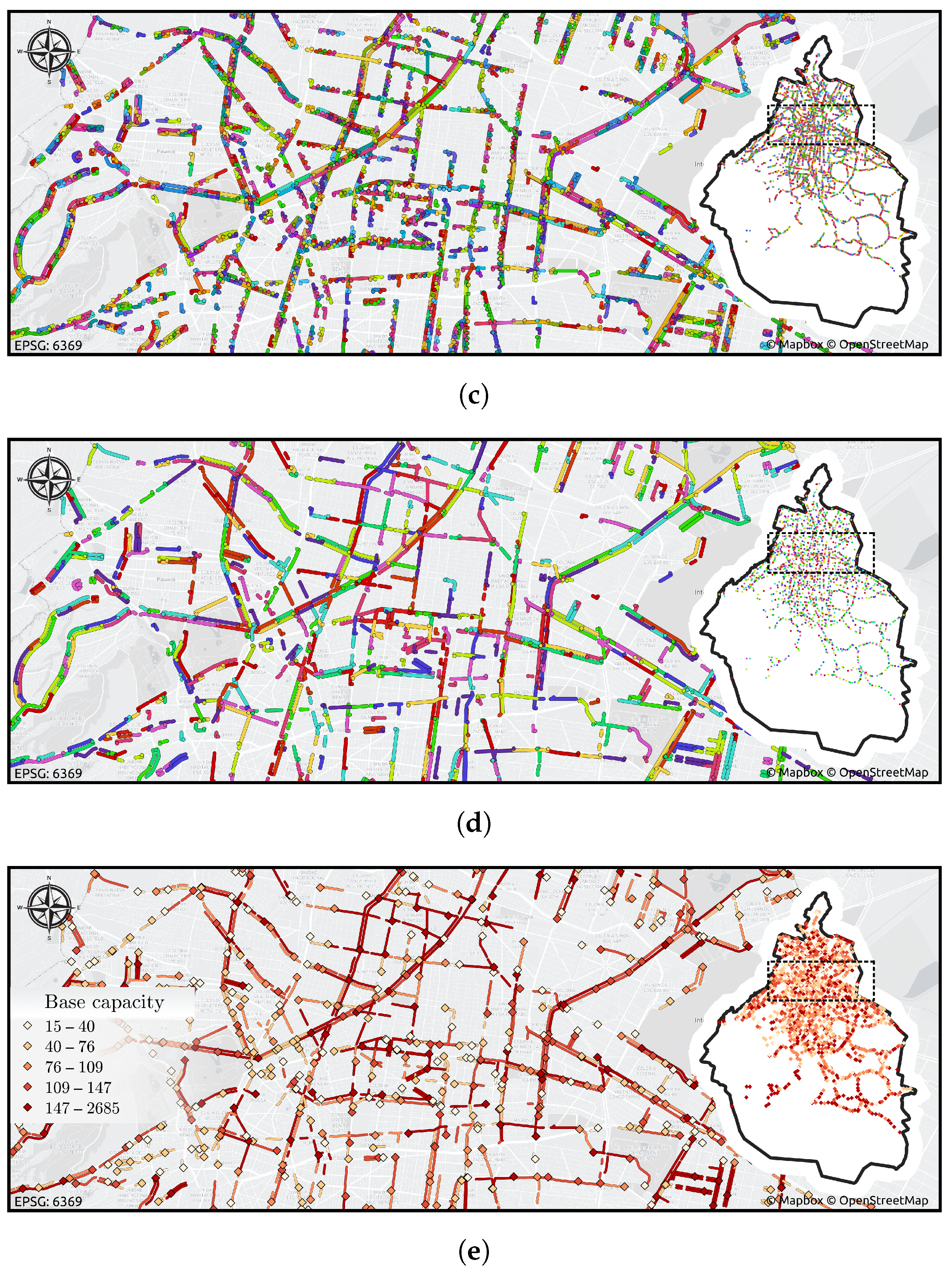
Process for obtaining candidate bases. (a) Selection by features, vertices, and resulting edges. (b) Selection by capacity, vertices, and resulting edges. (c) Redundancy elimination, representative vertices, and their associated edges. (d) Proximity grouping, representative vertices, and their associated edge groups. (e) Candidate bases colored by capacity.
Figure 7.
Kernel Density Estimation of buildings damaged by the 19 September 2017 earthquake.
Figure 8.
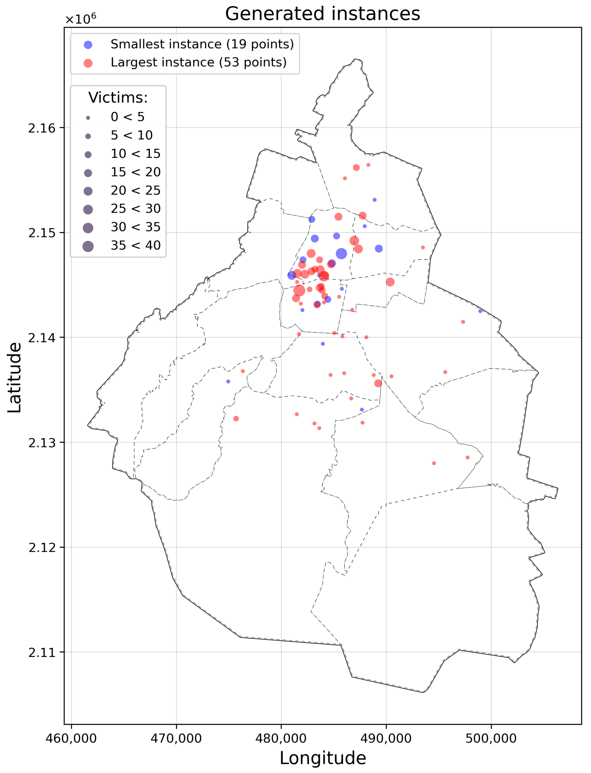
Instances with the lowest and highest number of demand points described in
Figure 7.
Figure 9.
Tiles used to determine the amount of traffic in Mexico City. Example of data obtained on 14 November 2023 at 13:45 h.
Figure 10.
Stages for obtaining traffic data using the TomTom API and the OSMNX network. (a) RGBA raster obtained through the TomTom API. (b) Conversion to single-band raster. (c) Sampling windows of the single-band raster. (d) Road network graph with traffic as attribute.
Figure 11.
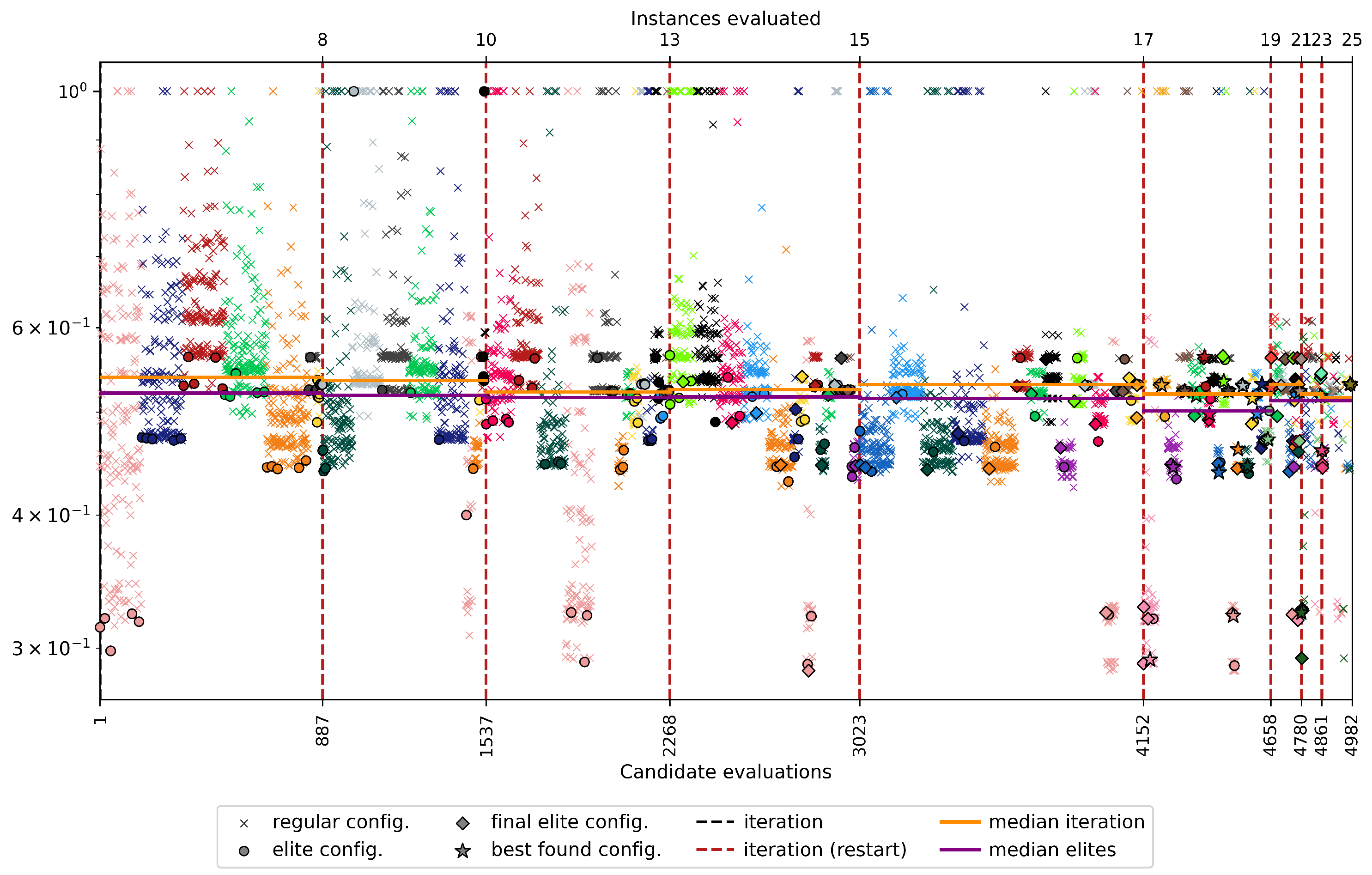
Experiments performed during parameter tuning. Each color represents a specific instance.
Figure 12.
Pareto front of 2017 earthquake post-disaster scenario.
Figure 13.
Preview of the solutions 1, 8, and 14 for the 2017 scenario.
Figure 14.
Interactive visualization of the solution, displaying the available layers and the default map view.
Figure 15.
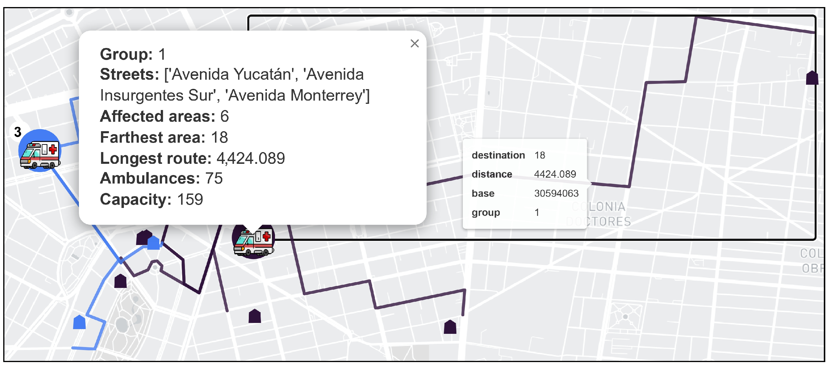
Elements of an activated base and a route. Only two specific groups are shown.
Figure 16.
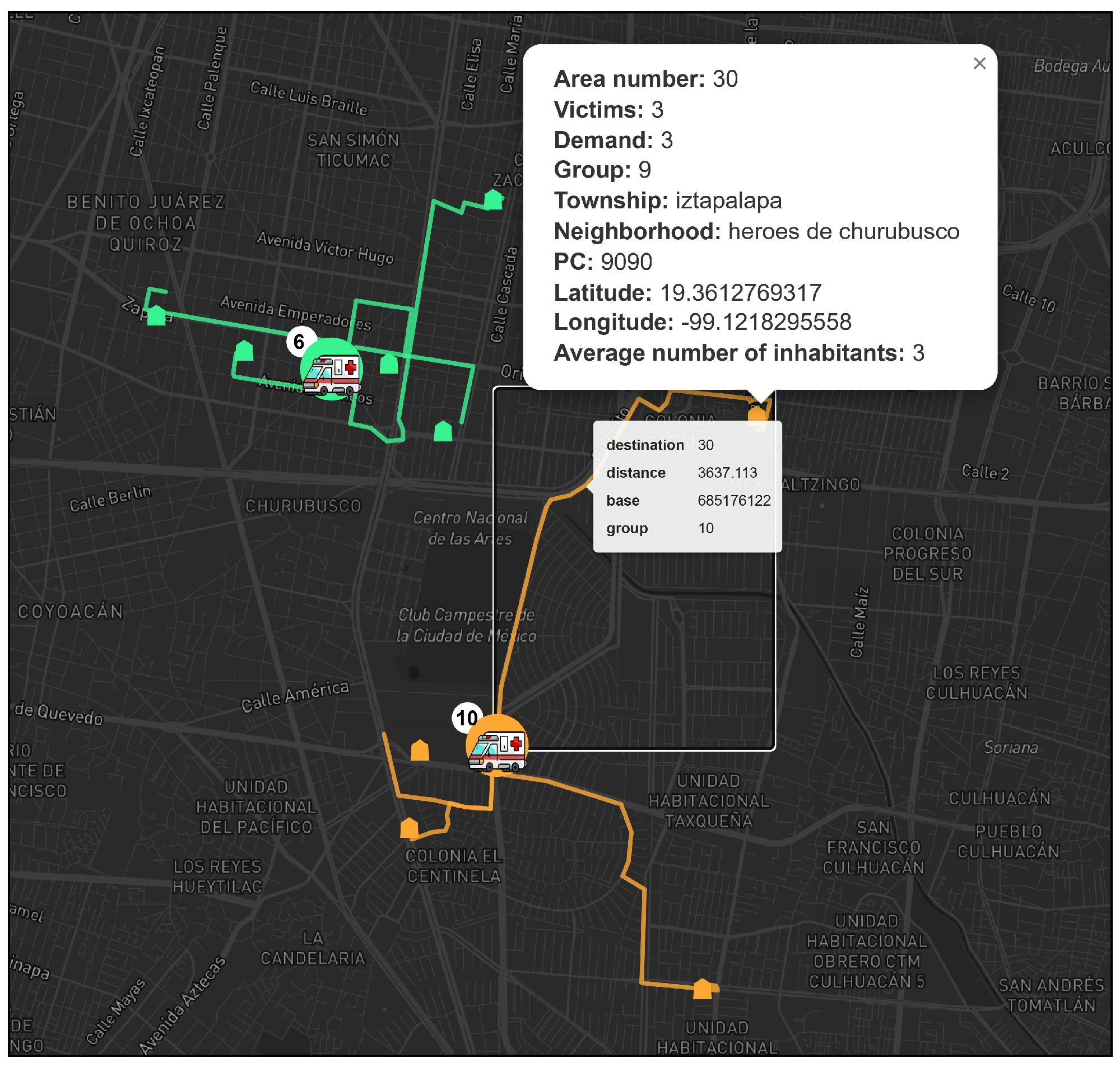
Elements of a demand point. Possible regions of attention are displayed.
Figure 17.
Comparison of the execution time of Dijkstra’s algorithm with NetworkX and Cugraph, ratio .
Figure 18.
Ratio of runtime to generate the instances between data reading, computation of the routes, and the remaining procedure.
Table 1.
Data retrieved from official data sources.
| Layer | Description | Geometry Type | Number of Records | Features |
|---|
| mayorships [31] | Geographic boundaries of each mayorship | polygon | 16 | 6 |
| risk_zones [32] | Earthquake risk zones | polygon | 4908 | 2 |
| regions * [33] | Classification of urban areas according to the unit responsible for rescue operations | polygon | 5 | 3 |
| hospitals [34] | Public and private hospitals operating in the CDMX | point | 584 | 59 |
| gathering_centers [35] | Emergency collection centers available | point | 67 | 10 |
| refuges [36] | Temporary emergency shelters available | pint | 67 | 10 |
| collapses [32] | Collapsed buildings from the 2017 earthquake | point | 38 | 1 |
| damages [32] | Damaged buildings from the 2017 earthquake | point | 38 | 1 |
| blocks [37] | Geographic delimitation of blocks and 2020 population census data | polygon | 1,215,066 | 18 |
| seduvi [38] | Buildings Centroid and their characteristics, provided by SEDUVI | point | 1,215,066 | 18 |
| land_registry [39] | Geographical delimitation of the buildings and their characteristics, provided by Land Registry Department | polygon | 1,607,109 | 7 |
Table 2.
Values used in the tuning phase for the values of the stop criteria.
| Parameter | Name | Values | Selected Value |
|---|
| Tolerance in the decision space | xtol | | |
| Tolerance in the target space | ftol | | |
| Criteria evaluation period | period | 100 | 100 |
| Ignore generations for criteria evaluation | n_skip | 100 | 100 |
| Maximum number of generations | n_max_gen | ≤10,000 | 500 |
| Maximum number of evaluations of items | n_max_evals | ≤10,000,000 | 100,000 |
Table 3.
Proposed values for algorithm parameters.
| Parameter | Name | Key | Type | Values |
|---|
| Crossover operator | crossover | –cr | categoric | un—cross uniform |
| hun—cross half uniform |
| Mutation operator | mutation | –mu | categoric | bf—bit flip mutation |
| bfo—active bit flip mutation |
| Allocation method | allocation | –a | categoric | cl—classic |
| ur—urgency-based |
| urc—demand–urgency-based |
| Repair method | repair | –rep | categoric | rn—normal repair |
| rm—repair with mutation |
| Population size | population | –pop | categoric 1 | (20, 50, 100, 200) |
| Percentage of offspring | offsprings | –dec | categoric 1 | (25, 50, 75) |
| Crossing percentage | prob_crossover | –prob_cr | categoric 1 | (0.5, 0.75, 0.9, 0.99) |
| Mutation percentage | prob_mutation | –prob_mu | categoric 1 | (0.5, 0.25, 0.1, 0.01) |
| Start probability | prob_initial | –prob_ini | categoric 1 | (0.25, 0.1, 0.01) |
Table 4.
Reducing transport network.
| Step | Result | Size |
|---|
| Transport network | | 128,825 |
| Selection by characteristics | | 15,560 |
| Selection by capacity | | 8184 |
| Elimination of redundancy | | 5784 |
| Proximity grouping | V | 1846 |
Table 5.
Response time to vertices from the closest candidate base, % = percentage of vertices covered in less than 9 min, p95 = maximum response time for of vertices (95th percentile), and = number of candidate bases that are discarded by level traffic .
| Daytime | | 20 km/h | 30 km/h | 40 km/h | 50 km/h | 60 km/h |
|---|
| | | % | p95 | % | p95 | % | p95 | % | p95 | % | p95 |
|---|
| 7:00 a.m. | 47 | 0.96 | 8.15 | 0.99 | 5.44 | 0.99 | 4.08 | 1.0 | 3.26 | 1.0 | 2.72 |
| 8:00 a.m. | 69 | 0.96 | 8.25 | 0.99 | 5.5 | 0.99 | 4.13 | 1.0 | 3.3 | 1.0 | 2.75 |
| 9:00 a.m. | 66 | 0.96 | 8.17 | 0.99 | 5.45 | 1.0 | 4.09 | 1.0 | 3.27 | 1.0 | 2.72 |
| 11:00 a.m. | 52 | 0.96 | 8.09 | 0.99 | 5.39 | 1.0 | 4.04 | 1.0 | 3.24 | 1.0 | 2.7 |
| 1:00 p.m. | 74 | 0.96 | 8.39 | 0.99 | 5.59 | 1.0 | 4.19 | 1.0 | 3.36 | 1.0 | 2.8 |
| 3:00 p.m. | 122 | 0.95 | 8.75 | 0.99 | 5.84 | 0.99 | 4.38 | 1.0 | 3.5 | 1.0 | 2.92 |
| 5:00 p.m. | 57 | 0.96 | 8.47 | 0.99 | 5.65 | 0.99 | 4.23 | 1.0 | 3.39 | 1.0 | 2.82 |
| 7:00 p.m. | 139 | 0.95 | 9.0 | 0.98 | 6.0 | 0.99 | 4.5 | 1.0 | 3.6 | 1.0 | 3.0 |
| 8:00 p.m. | 55 | 0.95 | 8.71 | 0.99 | 5.81 | 0.99 | 4.36 | 1.0 | 3.49 | 1.0 | 2.9 |
| 9:00 p.m. | 21 | 0.96 | 8.45 | 0.99 | 5.64 | 0.99 | 4.23 | 1.0 | 3.38 | 1.0 | 2.82 |
Table 6.
Characteristics of the instances created to describe demand points, : instance, : number of candidate bases that are discarded, : number of victims, d: demand.
| Date/Hour | | | | Total
| Min
| Max
| Min
| Max
|
|---|
| 0 | 27 October–09:00 a.m. | 319 | 1527 | 43 | 334 | 2 | 45 | 2 | 26 |
| 1 | 27 October–03:00 p.m. | 482 | 1364 | 45 | 463 | 2 | 45 | 2 | 19 |
| 2 | 28 October–11:00 a.m. | 265 | 1581 | 44 | 381 | 2 | 45 | 3 | 17 |
| 3 | 29 October–07:00 p.m. | 227 | 1619 | 38 | 515 | 2 | 45 | 2 | 67 |
| 4 | 30 October–1:00 p.m. | 240 | 1606 | 19 | 193 | 2 | 45 | 5 | 44 |
| 5 | 30 October–05:00 p.m. | 235 | 1611 | 53 | 570 | 2 | 45 | 2 | 16 |
| 6 | 31 October–07:00 a.m. | 306 | 1540 | 23 | 192 | 2 | 45 | 5 | 29 |
| 7 | 1 November–08:00 a.m. | 267 | 1579 | 37 | 275 | 2 | 45 | 3 | 16 |
| 8 | 1 November–08:00 p.m. | 280 | 1566 | 35 | 376 | 2 | 45 | 3 | 28 |
| 9 | 2 November–09:00 p.m. | 139 | 1707 | 26 | 302 | 2 | 45 | 2 | 34 |
Table 7.
List of parameters used in TomTom API.
| Parameter | Value |
|---|
| Zoom level | 16 |
| Total number of tiles (to cover the bounding box) | |
| Tiles occupied (intersecting the polygon of the CDMX) | 4789 |
| Meters per tile | |
| Meters per pixel | |
Table 8.
Values used for parameter tuning.
| Parameter | Value |
|---|
| Number of iterations | 10 |
| Performed experiments | 4982 |
| Remaining budget | 18 |
| Number of elites | 5 |
| Number of settings used | 679 |
| Total user time on CPU | 880,930.4 (10.19 days) |
Table 9.
Elite configurations.
| top | id | -cr | -mu | -a | -rep | -pop | -dec | -prob_cr | -prob_mu | -prob_ini |
|---|
| 1 | 625 | un | bf | ur | rm | 200 | 50 | 0.5 | 0.25 | 0.1 |
| 2 | 499 | un | bf | ur | rm | 200 | 50 | 0.75 | 0.5 | 0.25 |
| 3 | 432 | hun | bfo | ur | rm | 200 | 50 | 0.5 | 0.5 | 0.25 |
| 4 | 655 | un | bf | ur | rm | 200 | 50 | 0.5 | 0.5 | 0.1 |
| 5 | 617 | un | bfo | ur | rm | 200 | 50 | 0.5 | 0.5 | 0.1 |
Table 10.
Statistics of the Pareto front solutions of the 2017 scenario.
| Solution | | | | | * | | |
|---|
| 1 | 12,4065.2 | 6 | 7904.6 | 3264.9 | 1 | 2 | 16 |
| 2 | 10,5696.9 | 7 | 7800.3 | 2781.5 | 1 | 2 | 13 |
| 3 | 91,577.8 | 8 | 6107.8 | 2409.9 | 1 | 2 | 8 |
| 4 | 82,685.1 | 9 | 6258.1 | 2175.9 | 1 | 2 | 7 |
| 5 | 77,329.4 | 10 | 6258.1 | 2035.0 | 2 | 2 | 7 |
| 6 | 72,245.0 | 11 | 5013.1 | 1901.2 | 4 | 3 | 7 |
| 7 | 68,039.6 | 12 | 4907.8 | 1790.5 | 5 | 3 | 7 |
| 8 | 64,555.3 | 13 | 4907.8 | 1698.8 | 6 | 2 | 7 |
| 9 | 61,456.4 | 14 | 4907.8 | 1617.3 | 7 | 2 | 7 |
| 10 | 58,493.7 | 15 | 4907.8 | 1539.3 | 7 | 2 | 7 |
| 11 | 56,013.6 | 16 | 4907.8 | 1474.0 | 8 | 2 | 7 |
| 12 | 53,807.9 | 17 | 4907.8 | 1416.0 | 8 | 2 | 5 |
| 13 | 51,680.9 | 18 | 4907.8 | 1360.0 | 9 | 2 | 5 |
| 14 | 49,675.7 | 19 | 4907.8 | 1307.3 | 10 | 2 | 5 |
Table 11.
Runtime (in seconds) of the three main stages of data integration, : instance, avg: mean, std: standard deviation.
| | | | Reading | Processing | Dijkstra | |
|---|
| | | Avg | Std | Avg | Std | Avg | Std | Total |
| 0 | 1527 | 43 | 23.935 | 1.039 | 32.511 | 1.689 | 30.361 | 1.461 | 86.806 |
| 1 | 1364 | 45 | 24.452 | 1.208 | 32.973 | 1.449 | 30.775 | 1.199 | 88.2 |
| 2 | 1581 | 44 | 24.225 | 0.988 | 32.070 | 1.204 | 26.961 | 0.965 | 83.256 |
| 3 | 1619 | 38 | 23.358 | 0.235 | 31.373 | 0.569 | 22.408 | 0.137 | 77.139 |
| 4 | 1606 | 19 | 23.268 | 0.235 | 31.126 | 0.288 | 10.737 | 0.040 | 65.131 |
| 5 | 1611 | 53 | 22.983 | 0.178 | 30.961 | 0.361 | 30.305 | 0.165 | 84.249 |
| 6 | 1540 | 23 | 23.120 | 0.185 | 30.616 | 0.430 | 14.456 | 0.075 | 68.192 |
| 7 | 1579 | 37 | 22.946 | 0.200 | 30.621 | 0.434 | 22.071 | 0.110 | 75.638 |
| 8 | 1566 | 35 | 22.880 | 0.134 | 30.754 | 0.454 | 21.503 | 0.072 | 75.137 |
| 9 | 1707 | 26 | 22.869 | 0.182 | 30.295 | 0.438 | 14.182 | 0.053 | 67.345 |
| Disclaimer/Publisher’s Note: The statements, opinions and data contained in all publications are solely those of the individual author(s) and contributor(s) and not of MDPI and/or the editor(s). MDPI and/or the editor(s) disclaim responsibility for any injury to people or property resulting from any ideas, methods, instructions or products referred to in the content. |
© 2024 by the authors. Licensee MDPI, Basel, Switzerland. This article is an open access article distributed under the terms and conditions of the Creative Commons Attribution (CC BY) license (https://creativecommons.org/licenses/by/4.0/).
