On the Generalizability of Machine Learning Classification Algorithms and Their Application to the Framingham Heart Study

Abstract

The use of machine learning algorithms in healthcare can amplify social injustices and health inequities. While the exacerbation of biases can occur and be compounded during problem selection, data collection, and outcome definition, this research pertains to the generalizability impediments that occur during the development and post-deployment of machine learning classification algorithms. Using the Framingham coronary heart disease data as a case study, we show how to effectively select a probability cutoff to convert a regression model for a dichotomous variable into a classifier. We then compare the sampling distribution of the predictive performance of eight machine learning classification algorithms under four stratified training/testing scenarios to test their generalizability and their potential to perpetuate biases. We show that both extreme gradient boosting and support vector machine are flawed when trained on an unbalanced dataset. We then show that the double discriminant scoring of type 1 and 2 is the most generalizable with respect to the true positive and negative rates, respectively, as it consistently outperforms the other classification algorithms, regardless of the training/testing scenario. Finally, we introduce a methodology to extract an optimal variable hierarchy for a classification algorithm and illustrate it on the overall, male and female Framingham coronary heart disease data.

1. Introduction

As machine learning (ML) and artificial intelligence (AI) are rapidly proliferating in many aspects of decision-making in society, there is growing concern regarding their ethical use and their potential to perpetuate existing racial biases, as highlighted in predictive policing [1,2], in mortgage lending practices [3], in financial services [4] and in healthcare [5,6,7,8,9]. At the intersection of health, machine learning and fairness, a comprehensive review [10] of the ethical considerations that arise during the model development of machine learning in health has been laid out in five stages, namely problem selection, data collection, outcome definition, algorithm development and post-deployment considerations, the latter two of which are the main focus of this present research. For each of these five stages, there are considerations for machine learning to not only mitigate and/or prevent the exacerbation of existing social injustices, but also to attempt to prevent the creation of new ones. First, interest and available funding influence the selection of a research problem and this, together with the lack of diversity in the scientific workforce, leads to the exacerbation of existing global, racial and gender injustices [11,12,13]. Second, biases in data collection arise from two processes that result in a loss of data. On one hand, the type of collected data has been shown to suffer, at varying degrees, from challenges and limitations, as illustrated for randomized controlled trials [14,15,16], electronic health records [17,18,19] and administrative health records [20,21]. On the other hand, historically underserved groups, which include low- and middle-income nationals [22,23], transgender and gender-nonconforming individuals [24], undocumented immigrants [25] and pregnant women [26,27], are often underrepresented, misrepresented or missing from the health data that inform consequential health policy decisions. The third stage in the model pipeline is outcome definition, which may appear to be a straightforward healthcare task—for example, defining whether a patient has a disease—but, surprisingly, can be skewed by the prevalence of such disease and the way that it manifests in some patient populations. One such instance may occur during clinical diagnosis. For example, the outcome label for the development of cardiovascular disease could be defined through the occurrence of specific phrases in the clinical notes. However, women can manifest symptoms of acute coronary syndrome differently [28] and receive delayed care as a result [29]. In addition, ambiguities occur as a result of diagnosis codes being leveraged for billing purposes, rather than for clinical research [30]. Another instance in which outcome definition can lead to biases and the exacerbation of inequities is the use of non-reliable proxies to account for and predict a health outcome given that socioeconomic factors affect access to both healthcare and financial resources. The fourth stage in the model pipeline is algorithm development per se. Even when all considerations and precautions have been taken into account in the previous three stages to minimize the infiltration of biases, noise and errors in the data, the choice of the algorithm is not neutral and often is a source of obstruction to the ethical deployment of the algorithm. The crucial factors in model development are understanding confounding, feature selection, parameter tuning, performance metric selection and group fairness definition. Indeed, confounding features are those features that influence both the independent and dependent variables, and, as the vast majority of models learn patterns based on observed correlations within the training dataset, even when such correlations do not occur in the testing dataset, it is critical to account for confounding features, as illustrated in classification models designed to detect hair color [31] and in predicting the risk of pneumonia and hospital 30-day readmission [32]. Moreover, blindly incorporating factors like race and ethnicity, which are increasingly available due to the large-scale digitization of electronic health records, may exacerbate inequities for a wide range of diagnoses and treatments [33]. Therefore, it is crucial to carefully select the model’s features and to consider the human-in-the-loop framework, where the incorporation of automated procedures is blended with investigator knowledge and expertise [34]. Another crucial component of algorithm development is the tuning of the parameters, which can be set a priori, selected via cross-validation or extracted from a default setting from software. These methods that can lead to the overfitting of the model to the training dataset and a loss of generalizability to the target population, the latter of which is a central concern for ethical machine learning. To assess and evaluate a model, many performance metrics are commonly used, such as the area under the receiver operating characteristic curve (AUC) and area under the precision–recall curve (AUPRC) for regression models, on one hand, and the accuracy, true positive rate and precision for classification models, on the other hand. It is important to use a performance metric that reflects the intended use case and to be aware of potential misleading conclusions when using so-called objective metrics and scores [33]. Finally, the fifth stage of the model pipeline is the post-deployment of the model in a clinical, epidemiological or policy service. Robust deployment requires careful performance reporting and the auditing of generalizability, documentation and regulation. Indeed, it is important to measure and address the downstream impacts of models through auditing for bias and the examination of clinical impacts [35]. It is also crucial to evaluate and audit the deployment of its generalization, as any shift in the data distribution can significantly impact model performance when the settings for development and deployment differ, as illustrated in chest X-ray models [36,37,38]. While some algorithms have been proposed to account for distribution shifts post-deployment [39], their implementation suffers from significant limitations due to the requirement for the specification of the nature or amount of distributional shift, thus requiring tedious periodic monitoring and auditing. The last two components for the ethical post-deployment of machine learning are the establishment of clear and insightful model and data documentation and adherence to best practices and compliance with regulations. In addition, the introduction of complex machine learning models can sometimes lead to “black box” solutions, where the decision-making process is not transparent. Enhancing the clinical interpretability of the algorithms, possibly through the integration of explainable AI (XAI) techniques, could increase their acceptance among healthcare professionals. Providing insights into how and why predictions are made can aid in clinical decision-making, fostering trust and facilitating the adoption of these models in medical practice.

In [40], a review of 2815 research articles from the MEDLINE, Embase, Web of Science, ClinicalTrials.gov and ICTRP databases pertaining to the prediction of atrial fibrillation, which is a major risk factor for stroke, identified sixteen studies using machine learning models to predict incident atrial fibrillation and three studies focusing on machine learning models to detect atrial fibrillation post-stroke. It concluded that (1) many models used only a limited number of variables available in the patients’ health records; (2) only 37% were externally validated, and a stratified analysis was often lacking; (3) 0% of the models and 53% of the datasets were made available, which limited the transparency and reproducibility; and (4) there were no sufficient details to ensure bias mitigation. As such, the study identified the low generalizability, high false alarm rate and the lack of interpretability as additional factors that need to be addressed before a machine learning model can be widely deployed in a clinical care setting, and it recommends the improvement of the generalizability and the reduction of potential systemic biases, as well as investing in external validation studies whilst developing a transparent pipeline to ensure reproducibility.

With the algorithm development and post-deployment considerations of the five-stage model pipeline [10] on one hand, and with the improvement of the generalizability recommended in [40] on the other hand, this research uses the well-known Framingham coronary heart disease data as a case study and focuses on the comparison of several classification algorithms, in a paired design setting, using electronic health records, with the goal of identifying a methodology that is not only ethical, robust and understandable by practitioners or community members but also generalizable. While regression models for dichotomous observations are widely used by modelers, the probability outcome for patient-level data may not be insightful or helpful to determine whether a given patient should undergo further intervention, i.e., whenever the response of a practitioner to a patient (or family member) is expected to be a binary response rather than a vague probability statement. Despite the fact that this research was conducted before the publication of [40], the relevance of our comparative analysis is its response to one of the limiting factors highlighted in [40], which is the lack of performance benchmarking against conventional predictive models, with the majority of the atrial fibrillation studies (10/16) utilizing only one model architecture, without comparing the performance of machine learning models against baseline models such as logistic regression. Our study compares several machine learning algorithms in a paired design framework with a high number of cross-validation steps across several stratified training/testing scenarios, using the same data and set of variables. In Section 2, we recall the historical context of the Framingham Heart Study, and we then describe the seven predictors and the four training/testing scenarios used in this comparative analysis. We also recall the definitions of commonly used performance metrics for classification algorithms, i.e., the accuracy, true positive rate (sensitivity) and true negative rate (specificity). We then make the distinction between positive precision (resp., observed prevalence), which is simply called precision (resp., prevalence) in the literature, and negative precision (resp., predicted prevalence), which we introduce and define. Finally, we introduce the classification performance matrix as an extension of the confusion matrix with these seven performance metrics (accuracy, true positive/negative rates, positive/negative precision and observed/predicted prevalence) as a comprehensive and transparent means of assessing and comparing the machine learning algorithms. 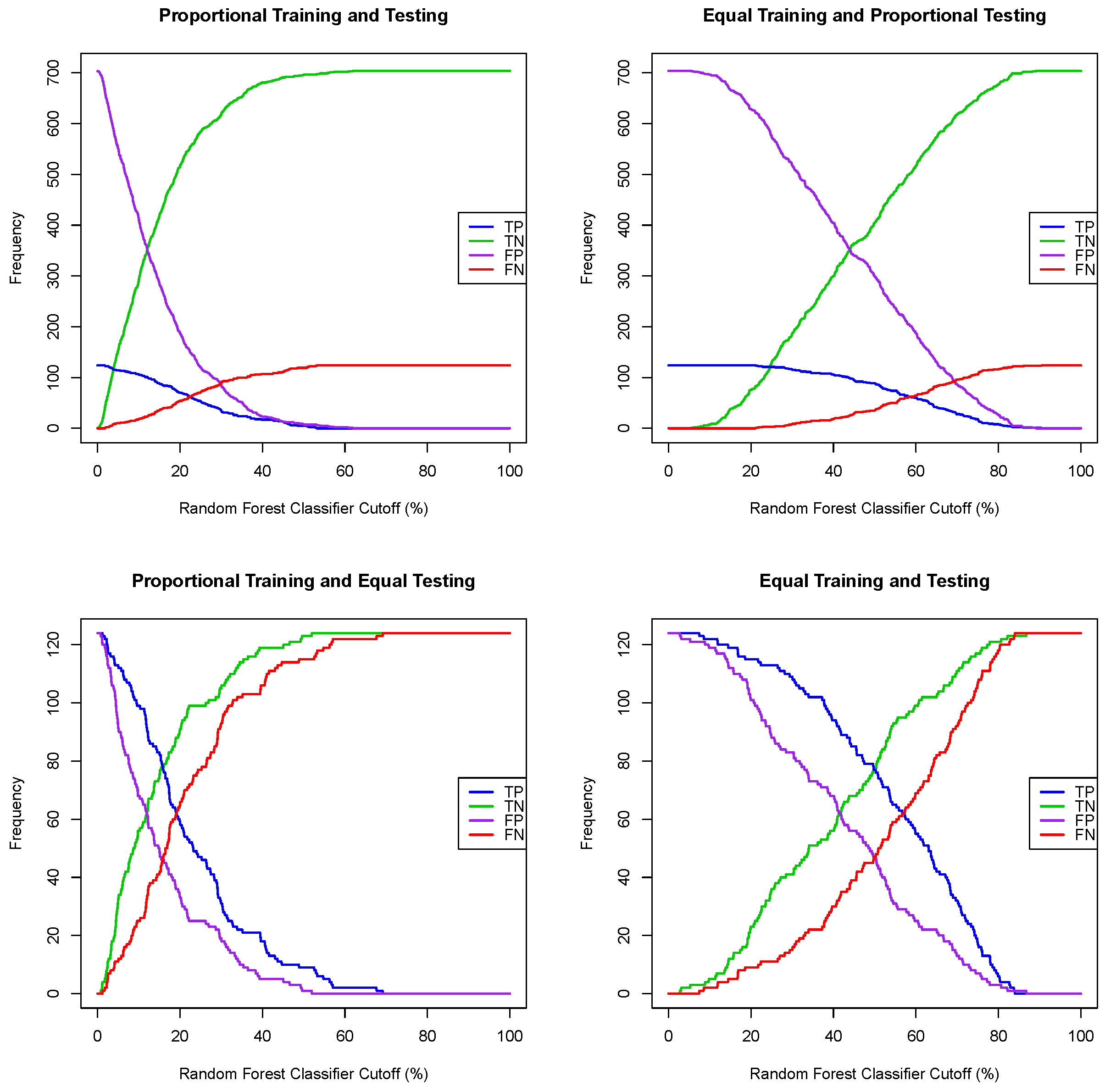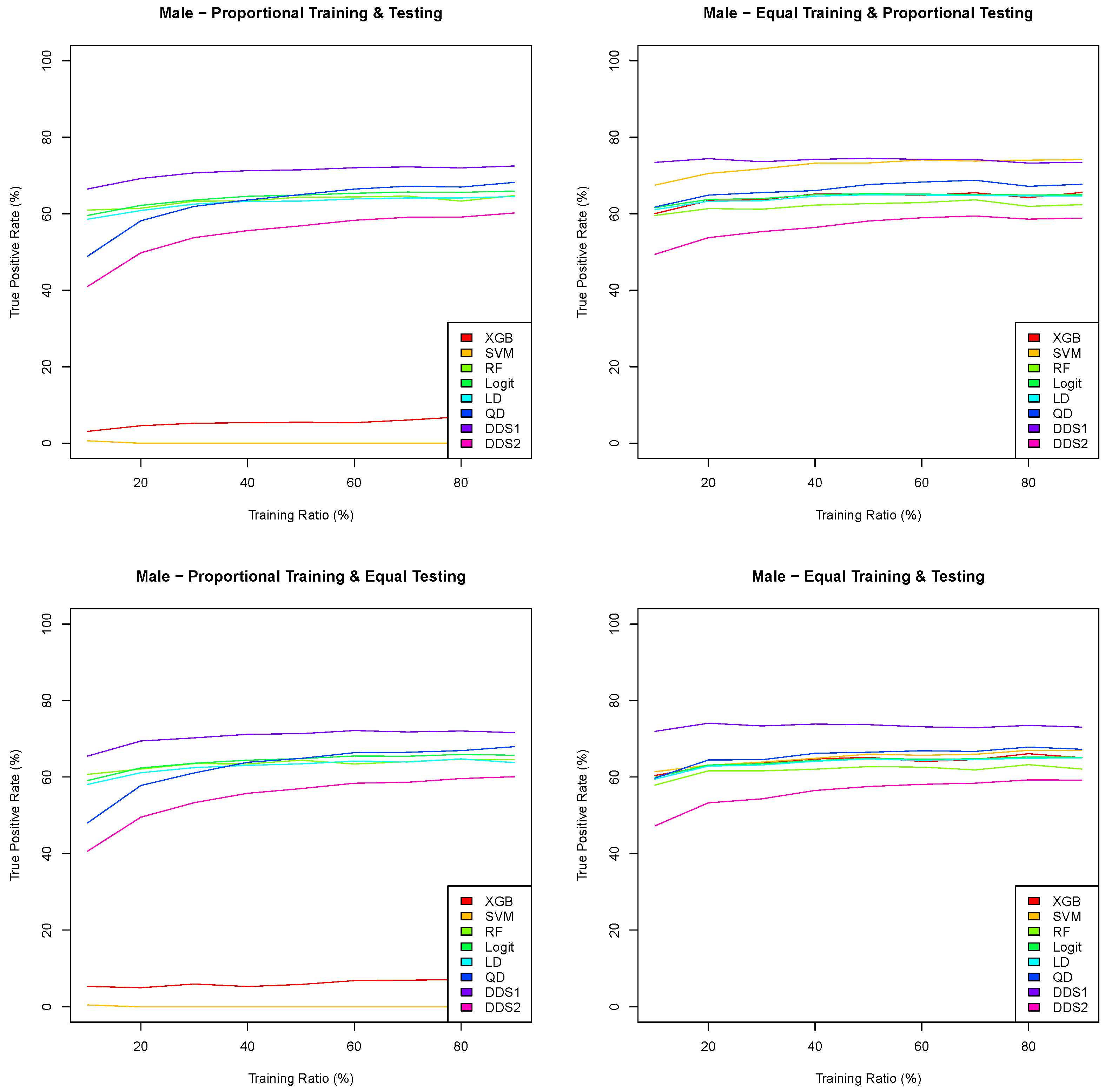In Section 3, we not only show that the naive choice of a 50% probability cutoff to convert a regression algorithm for dichotomous observation into a classification algorithm leads to misclassification, but we show also how a balanced and optimal probability cutoff can be determined to effectively convert logistic [41] and random forest [42] regression models into classifiers. We investigate also the effect of using the significant variables of a logistic regression model on the classification performance. We then compare the performance of eight classification algorithms, two of which are widely used supervised machine learning algorithms, namely extreme gradient boosting (XGB) [43] and support vector machine (SVM) [44], together with the logistic and random forest classifiers and two uncommonly used supervised machine functions, i.e., linear and quadratic discriminant functions [45]. We introduce two different combinations of the linear and quadratic discriminant functions into two scoring functions, which we call the double discriminant scoring of types 1 and 2. Using a paired design setup, we perform a sampling distribution analysis for these eight classification algorithms under four different training/testing scenarios and for varying training/testing ratios. We determine, from the comparison of the performance sampling distributions, the algorithm that consistently outperforms the others and is the least sensitive to distributional shifts. We then lay out and illustrate a methodology to extract an optimal variable hierarchy, i.e., a sequence of variables that provides the most robust and most generalizable variable selection for the classification algorithm for a given performance metric. For instance, if the optimal variable hierarchy for a classification algorithm and a performance metric is a sequence of two variables, then the first variable is the optimal single variable among the set of all features, the first and second variables constitute the optimal pair of variables among all pairs of features and the inclusion of any extra feature in this two-variable hierarchy would diminish the performance metric. We show in particular that the optimal variable hierarchy of the double discriminant scoring of type 1, with respect to the true positive rate and applied to the Framingham coronary heart data, satisfies the Bellman principle of optimality, leading then to the reduction of the sampling distribution tests from $2^p-1$ iterations to at most $p(p+1)/2$, where p is the number of variables (features). This methodology is applied to the entire Framingham CHD data and to both the male and female Framingham CHD data. Finally, in Section 4, we discuss the findings of the comparative analyses and summarize the strengths and limitations of our study.

2. Materials and Methods

The Framingham Heart Study is a widely acknowledged longitudinal cohort study [46,47,48,49]. Motivated by the serious epidemic of cardiovascular disease (CVD) in the 1950s, becoming the leading cause of death and the reason that the population’s life expectancy beyond age 45 did not increase, action was needed to identify the determinants of the disease process. Given that no treatment capable of prolonging life for those who survived an attack existed, a preventive approach was deemed more important than a search for a cure. Moreover, given that CVD is a disease that develops over time, a longitudinal study was necessary. The Framingham Study [46,49] was conducted as follows: a systematic sample of 2 of every 3 families in the town of Framingham, Massachusetts, was selected. People in these families, between the ages of 30 and 59 years, were invited to participate in the study. A total of 5209 individuals (2336 men and 2873 women) joined the study, with the goal of collecting epidemiological data on CVD and the establishment of the relations among risk factors such as clinical (age, sex, blood pressure, cholesterol, body weight and diabetes), and lifestyle (smoking, physical activity and alcohol consumption) parameters. The participants of the Framingham Heart Study were continuously monitored to identify when a CVD event occurred. Given the success of the Framingham Heart Study, a second cohort in 1971, with over 5000 subjects, and a third cohort in 2001, with over 4000 subjects, led to two replications [50,51]. The reader may refer to [49] for the most recent review of the Framingham Heart Study and an overview of the Framingham risk functions for CVD and coronary heart disease (CHD). Note that CHD includes myocardial infarction (i.e., heart attack), coronary death, stroke and heart failure.

Using the Framingham coronary heart disease data available on Kaggle, we extracted a sub-dataset consisting of seven explanatory variables, representing, for each patient, the age $X_1$, total cholesterol $X_2$, systolic blood pressure $X_3$, diastolic blood pressure $X_4$, body mass index (BMI) $X_5$, heart rate $X_6$ and number of cigarettes smoked per day $X_7$, and one dichotomous response variable Y, representing whether a patient had coronary heart disease in the 10-year period following the measurement of these seven explanatory variables. The sub-data extracted, which we refer to as the Framingham CHD data in this paper, consisted of all patients for which there were no missing measurements for each of the seven explanatory variables. The goal of this study was to compare the sampling distribution of the performance of several machine learning classification algorithms under several training/testing scenarios to (1) determine a methodology that can better predict whether (or not) a patient will develop coronary heart disease in the 10-year period following the measurement of the seven explanatory variables; (2) determine the best way to train these machine learning algorithms and their sensitivity to both the size and the distribution of the training datasets; and (3) extract an optimal variable hierarchy for the explanatory variables and assess their generalizability to new medical and geographical data. The characteristics of patients who had coronary heart disease ten years later are given in

Table 1. Characteristics of patients who had coronary heart disease ten years later.

Male + Female	CHD	No CHD
Total, n, (%)	622 (15.02)	3520 (84.98)
Age, $X_1$, mean (SD)	54.20 (7.98)	48.72 (8.39)
Total Cholesterol, $X_2$, mean (SD)	245.89 (48.05)	235.08 (43.74)
Systolic Blood Pressure, $X_3$, mean (SD)	143.52 (26.58)	130.31 (20.41)
Diastolic Blood Pressure, $X_4$, mean (SD)	87.00 (14.09)	82.18 (11.28)
Body Mass Index, $X_5$ mean (SD)	26.52 (4.50)	25.67 (3.99)
Heart Rate, $X_6$, mean (SD)	76.54 (12.29)	75.71 (11.99)
Number of Cigarettes Smoked Per Day, $X_7$, mean (SD)	10.73 (13.07)	8.68 (11.68)

.

These Framingham CHD data consisted then of two groups: Group 1, with $N_1=622$ patients who had coronary heart disease in the 10-year period following the beginning of the study, and Group 2, with $N_2=3520$ patients who did not have coronary heart disease in the same 10-year period. The prevalence of CHD in these data was $15\%$, meaning that 15% of the $N=N_1+N_2=4142$ patients had coronary heart disease. Data analysts often randomly split the data into training and testing datasets using a training ratio $\tau$. For instance, if one assigns randomly 80% of the data to the training dataset, and then assigns the remaining 20% of the data to the testing dataset, then the training ratio is $\tau =0.8$. Given a training ratio of $\tau =0.8$, there are several ways to split the data into training and testing sets, the simplest of which is to merge Group 1 and Group 2 and then randomly split the data into training and testing datasets using a given training ratio $\tau$. This simple splitting leads to the overrepresentation in the training dataset of the largest of the two groups, i.e., Group 2 in these Framingham CHD data. For reasons that will be clarified in the findings in Section 3.2, we do not consider this simple splitting in this paper, but rather the following four stratified training/testing scenarios. Let us denote by $n_1$ the number of observations in the intersection of Group 1 and the training dataset, by $n_2$ the number of observations in the intersection of Group 2 and the training dataset and by $n_3$ the number of observations used in the testing dataset. Therefore, the number of observations in the training dataset is $n_1+n_2$. In what follows, $[.]$ denotes the rounding to the nearest natural number. For a fixed training ratio $\tau$, let us consider the following four training/testing scenarios.

• Proportional training and testing: randomly select $n_1=\left[\tau N_1\right]$ observations from Group 1 and $n_2=\left[\tau N_2\right]$ observations from Group 2 to form the training dataset, and then use the remaining $n_3=\left[(1-\tau )(N_1+N_2)\right]$ observations for the testing dataset.
• Equal training and proportional testing: randomly select $n_1=n_2=[\tau min(N_1,N_2)]$ observations from each of Groups 1 and 2 to form the training dataset and then select the remaining $(1-\tau )N_1$ observations of Group 1 and randomly select $(1-\tau )N_2$ observations from the remaining observations of Group 2 to form the testing dataset of size $n_3=\left[(1-\tau )(N_1+N_2)\right]$.
• Proportional training and equal testing: randomly select $n_1=\left[\tau N_1\right]$ observations from Group 1 and $n_2=\left[\tau N_2\right]$ observations from Group 2 to form the training dataset; then, randomly select $(1-\tau )min(N_1,N_2)$ from each of Groups 1 and 2 to form the testing dataset and hence $n_3=2(1-\tau )min(N_1,N_2)$.
• Equal training and testing: randomly select $n_1=n_2=[\tau min(N_1,N_2)]$ from each of Groups 1 and 2 to form the training dataset; then, to form the testing dataset, randomly select $[(1-\tau )min(N_1,N_2)]$ observations from the remaining observations for each of Groups 1 and 2 and hence $n_3=2[(1-\tau )min(N_1,N_2)]$.

Using the Framingham CHD data, where $N_1=622$, $N_2=3520$ and with a training ratio $\tau =0.8$, the sizes $n_1$, $n_2$ and $n_3$ for each of the four training/testing scenarios are given in

Table 2. Training and testing dataset sizes across four training/testing scenarios and for a training ratio $\tau =0.8$.

Training	Testing	${\mathit{n}}_1$	${\mathit{n}}_2$	${\mathit{n}}_3$
Proportional	Proportional	498	2819	124 + 704 = 828
Equal	Proportional	498	498	124 + 704 = 828
Proportional	Equal	498	2819	124 + 124 = 248
Equal	Equal	498	498	124 + 124 = 248

.

Once a classification model has been tested, one can produce the confusion matrix, i.e., a table specifying the frequencies of the true positive (TP), the false positive (FP), the false negative (FN) and the true negative (TN) predictions. One can then use this confusion matrix to compute one or several performance metrics to assess the classification model, such as the accuracy, true positive rate (sensitivity), true negative rate (specificity) and precision. In what follows, we recall the definitions (and formulas) of the accuracy and true positive and true negative rates. We then introduce and make a distinction between positive precision and negative precision on one hand, and between the observed prevalence and the expected prevalence on the other hand. Finally, we introduce the classification performance matrix as an extension of the standard confusion matrix, along with the above seven model performance metrics. Let us refer to the total number of predictions as the grand total, i.e., $\mathrm{grand}\mathrm{total}=\mathrm{TP}+\mathrm{FP}+\mathrm{FN}+\mathrm{TN}$. Recall that the accuracy (Acc) of a classification model is the ratio of correct predictions among the total number of predictions, i.e., $Acc=(TP+TN)/\mathrm{grand}\mathrm{total}$. Recall also that the true positive rate (TPR), also called sensitivity in the literature, is the ratio of the number of true positive predictions among the total number of actual positive tested cases, i.e., $TPR=TP/(TP+FN)$. Finally, recall that the true negative rate (TNR), also called specificity in the literature, is the ratio of the number of true negative predictions among the total number of actual negative tested cases, i.e., $TNR=TN/(FP+TN)$. We define the positive precision (PPrec), which is simply called precision in the literature, as the ratio of the number of true positive predictions among the total number of tested cases that have been predicted as positive by the classification model, i.e., $PPrec=TP/(TP+FP)$. Similarly, we define the negative precision (NPrec) as the ratio of the number of true negative predictions among the total number of tested cases that have been predicted as negative by the classification model, i.e., $NPrec=TN/(FN+TN)$. We define the observed prevalence (OPrev), which is simply called prevalence in the literature, as the proportion of positive cases among the tested cases, i.e., $OPrev=(TP+FN)/\mathrm{grand}\mathrm{total}$. Finally, we define the expected prevalence (EPrev) as the ratio between the number of tested cases that have been predicted as positive among the tested cases, i.e., $EPrev=(TP+FP)/\mathrm{grand}\mathrm{total}$. Lastly, we introduce an extension of the confusion matrix with the above seven performance metrics to provide a practical and comprehensive way to compare the performance of several classification algorithms across the four training/testing scenarios. We believe that this classification performance matrix (

Table 3. Classification performance matrix.

		Predicted
		Positive	Negative	Total	True Rate %
Actual	Positive	TP	FN	TP + FN	TPR
	Negative	FP	TN	FP + TN	TNR
	Total	TP + FP	FN + TN	Grand Total	OPrev
	Precision %	PPrec	NPrec	EPrev	Acc

) is comprehensive and transparent as it allows us, at a glance, to detect whether a classification model is biased and flawed. For instance, if the prevalence of the testing dataset is high, e.g., 95%, then a classification model that predicts all tested cases as positive would have 95% accuracy and a 100% true positive rate. A modeler that uses only these two metrics to build and/or compare models would have a false impression of obtaining a successful model. However, this model would be flawed, as the true negative rate would be 0%, which means that all tested cases that are negative would be predicted as positive, and thus it would trigger, in a medical context, additional interventions that are financially, timely and emotionally costly, rendering the practical implementation of this model ineffective.

3. Results

3.1. Logistic and Random Forest Classifiers

Given a regression model for a dichotomous random variable, e.g., a logistic regression or random forest, where the output for one tested case is the probability of being a positive case, one can convert such a regression model into a classification algorithm by choosing a probability threshold or a classifier cutoff, and then classify a tested patient as positive if the output of the regression model is greater or equal than the chosen classifier cutoff and classify a tested patient as negative otherwise. A naive classifier cutoff of 50% leads to poor prediction performance when the prevalence of the training dataset deviates substantially from 50%. Indeed, for each of the four training/testing scenarios, the Framingham CHD data, with all seven explanatory variables, were split (one simulation) using a training ratio of $\tau =0.8$. Both logistic regression and random forest models were extracted using the training dataset, and then, using both models, all patients in the testing data set were classified using successive values of a classifier cutoff ranging from $0\%$ to $100\%$, with a 1% step, and the number of true/false positive and true/false negative cases was recorded. The graphs of the true positive, false positive, false negative and true positive cases as functions of the classifier cutoff for each training/testing scenario, and for both the logistic and random forest regression models, are given in Figure 1 and Figure 2. A good classifier cutoff should minimize misclassification. As the classifier cutoff increases, the number of true negatives (TN, green curve) increases, and the number of true positives (TP, blue curve) decreases. Thus, an equilibrium classifier cutoff must strike a balance between the number of true positive and the number of true negative cases. One can observe from each of the logistic and random forest graphs that such a balanced classifier cutoff is around 15% when the training dataset is proportional (first and third training/testing scenarios), and it is around 50% when the training dataset is equal (second and fourth training/testing scenarios). In other words, a good and balanced classifier cutoff for both the logistic and random forest regression models appears to be the prevalence of the training dataset, independent of the prevalence of the testing dataset. In light of this observation, we replicated the above simulation one hundred times and superposed the graphs of each simulation into the same graph, as shown in Figure 3 and Figure 4. For these sampling distributions, the yellow dots represent the average points of intersection (centroïd) of the 100 pairs of curves, TN–TP, TP–FN, FN–FP and TN–FP. The black dot is the average point (centroïd) of the four yellow points. For these sampling distributions (100 simulations), the equilibrium classifier cutoff for the logistic regression, i.e., the x-coordinate of the black dot, is 15.56% (resp., 47.48%, 15.25 and 50.03%) for the proportional training and testing scenario (resp., equal training + proportional testing, proportional training + equal testing and equal training + testing). Similarly, the equilibrium classifier cutoff for the random forest regression, i.e, the x-coordinate of the black dot, is 16.47% (resp., 48.77%, 16.14 and 50.70%) for the proportional training and testing scenario (resp., equal training + proportional testing, proportional training + equal testing and equal training + testing). In light of these sampling distributions, we propose to chose the equilibrium classifier cutoff for both the logistic and random forest regression models to be the prevalence of the training dataset. These results are coherent with the findings in [52], pertaining to machine learning models for acute kidney injury risk stratification in hospitalized patients. In this study [52], penalized logistic regression using the least absolute shrinkage and selection operator (LASSO), random forest and a gradient boosting machine were trained to predict risk of acute kidney injury using electronic medical record data available at 24 h of inpatient admission. Moreover, the performance of the three algorithms in [52] was evaluated using the area under the receiver characteristic curve (AUROC) and precision–recall curves, and the probability cutoff was determined based on Youden’s index from 5% to 95% with a 5% step. It was found that a probability cutoff greater than 15% provided sensitivity of 0.80 and 0.79. In light of our study, with 100 cross-validations and a probability cutoff range of 0% to 100% with a 1% step, we believe that the 15% optimal probability cutoff in [52] was due to the prevalence of the training data, where the training cohort comprised electronic health record admissions from 2012 through 2017, with a testing cohort composed of electronic health record admissions in 2018.

Note that all above testing for both the logistics and random forest regression models was performed using all seven explanatory variables. One can justifiably argue that using all explanatory variables may not lead to optimal models, and thus one may question the use of such a balanced classifier cutoff. To test this hypothesis, we performed one thousand logistic regression model analyses for each of the four training/testing scenarios, and we counted, for each of the intercepts and the seven explanatory variables, the number of times such a variable was significant, using a significance level $\alpha$ of 1%, 5% and 10%. The results of these 1000 simulations (cross-validation) are summarized in

Table 4. Logistic regression variable significance analysis for four training/testing scenarios—1000 simulations.

$\mathit{\alpha }$	Training	Testing	${\mathit{X}}_0$	${\mathit{X}}_1$	${\mathit{X}}_2$	${\mathit{X}}_3$	${\mathit{X}}_4$	${\mathit{X}}_5$	${\mathit{X}}_6$	${\mathit{X}}_7$
1%	Proportional	Proportional	1000	1000	2	1000	0	0	0	1000
	Equal	Proportional	1000	1000	21	622	0	5	0	1000
	Proportional	Equal	1000	1000	4	1000	0	0	0	1000
	Equal	Equal	1000	1000	21	656	2	7	1	1000
5%	Proportional	Proportional	1000	1000	82	1000	0	25	2	1000
	Equal	Proportional	1000	1000	125	887	15	69	19	1000
	Proportional	Equal	1000	1000	71	1000	0	18	0	1000
	Equal	Equal	1000	1000	130	883	15	62	15	1000
10%	Proportional	Proportional	1000	1000	185	1000	1	73	12	1000
	Equal	Proportional	1000	1000	257	953	43	150	18	1000
	Proportional	Equal	1000	1000	207	1000	1	56	6	1000
	Equal	Equal	1000	1000	228	941	43	124	32	1000

, where $X_0$ stands for the logistic regression intercept.

For all three significance levels $\alpha$, the y-intercept, age $X_1$ and number of cigarettes smoked per day $X_7$ were statistically significant 1000 times (out of 1000). Moreover, systolic blood pressure $X_3$ was statistically significant 1000 times when the testing dataset was proportional (15% prevalence) and between 622 and 953 times when the testing dataset was equal (50% prevalence). For a significance level of $\alpha =10\%$, the total cholesterol level $X_2$ was statistically significant between 185 and 257 times (out of 1000), which was roughly between 20 and 25% of the 1000 simulation runs. In light of this logistic regression variable significance analysis, for each of the four training/testing scenarios and for the same data split (training ratio $\tau =0.8$), we implemented three logistic regression models: Logistic Model 1 with all seven explanatory variables; Logistic Model 2 with only age $X_1$, systolic blood pressure $X_3$ and the number of cigarettes smoked per day $X_7$; and Logistic Model 3 with the total cholesterol $X_2$ added to the three variables in Model 2. For a given training/testing scenario and for the same data split, the three logistic regression models were converted into three logistic classifiers using a balanced/equilibrium classifier cutoff equal to the prevalence of the training dataset, and the number of true positive cases (out of 124 patient tests for each training/testing scenario) was recorded. This process was repeated 1000 times, and the average number of true positive predictions for each of the three regression classification models is summarized in

Table 5. Average number of true positive cases (out of 124) for three logistic classification models across four training/testing scenarios—1000 simulations.

Training	Testing	Logistic 1 $({\mathit{X}}_{\mathbf{1}},\cdots ,{\mathit{X}}_{\mathbf{7}})$	Logistic 2 $({\mathit{X}}_{\mathbf{1}},{\mathit{X}}_{\mathbf{3}},{\mathit{X}}_{\mathbf{7}})$	Logistic 3 $({\mathit{X}}_{\mathbf{1}},{\mathit{X}}_{\mathbf{2}},{\mathit{X}}_{\mathbf{3}},{\mathit{X}}_{\mathbf{7}})$
Proportional	Proportional	81.80	81.81	82.59
Equal	Proportional	82.68	82.80	83.06
Proportional	Equal	81.85	82.80	82.67
Equal	Equal	82.18	81.77	82.73

.

Table 5 shows that the number of true positive predictions is roughly the same regardless of which variables are used for the logistic regression. In other words, while different choice of variables may lead to differences in the logistic regression where the outcome is a probability, such a variable choice appears not to be relevant for a logistic classifier across all four training/testing scenarios, with an (equilibrium) classifier cutoff equal to the prevalence of the training dataset. A modeler can thus either use all variables or run a few simulation runs and use the subset of variables that are statistically significant for the logistic regression. Finally, the average numbers of true negatives, false positives and false negatives were consistent with the results in Table 5, and thus we choose not to report the average frequencies.

3.2. Training Ratio Analysis and Classification Algorithm Comparison

We consider, in this subsection, the following eight classification algorithms, and we compare their predictive performance using the Framingham CHD data across the four training/testing scenarios in a paired-design-type setting. Note that the last two classification algorithms, i.e., the double discriminant scoring of type 1 and type 2, are introduced in this paper and have not been considered yet in the literature.

• Extreme gradient boosting (XGB), for which the outcomes for one tested case are the two probabilities of being a positive and negative case, respectively. Therefore, we assign a tested case to Group 1 (having CHD) if the probability of being positive is greater than the probability of being negative; otherwise, we assign the tested case to Group 2 (not having CHD).
• Support vector machine (SVM).
• Random forest classifier (RF), where the classifier cutoff is set to be the prevalence of the testing dataset (as shown in Section 3.1).
• Logistic classifier (Logit), where the classifier cutoff is set to be the prevalence of the testing dataset (as shown in Section 3.1), and the link function is the logit function.
• Linear discriminant function (LD).
• Quadratic discriminant function (QD).
• Double discriminant scoring of type 1 (DDS1), where a tested patient is assigned to Group 1 (having CHD) if either the linear or quadratic discriminant models assigns the tested patient to Group 1; otherwise, the tested patient is assigned to Group 2 (not having CHD).
• Double discriminant scoring of type 2 (DDS2), where a tested patient is assigned to Group 1 (having CHD) if both the linear and quadratic discriminant models assign the tested patient to Group 1; otherwise, the tested patient is assigned to Group 2 (not having CHD).

Note that both the linear and quadratic discriminant functions [45] in this research assume normality and are derived as the difference in the log-likelihood function. When the (multivariate) population variances of Groups 1 and 2 are assumed to be equal (resp., different), the maximum log-likelihood discriminant rule leads to the linear (resp., quadratic) discriminant function. We choose to simply consider both instances without running a Bartlett test. One can consider the double discriminant scoring of type 1 (resp., type 2) as a “liberal” (resp., “conservative”) combination of the linear and quadratic discriminant functions. We compare the mean predictive performance of these eight classification algorithms for a training ratio $\tau =0.1,0.2,\cdots ,0.8,0.9$ across the four training/testing scenarios, using 100 simulations for each classification algorithm. All predictive performance metrics in the classification performance matrix in Table 3, i.e., TP, FP, FN, TN, TPR, TNR, PPrec, NPrec, OPrev, EPrev and Acc, are recorded, and the means of 100 simulations are computed for each one of the four training/testing scenarios. In Figure 5, the graphs of the true positive rates as a function of the training ratio $\tau$ are plotted, and they lead to the following remarks. First, both the extreme gradient boosting and support vector machine classification algorithms perform poorly when the training dataset is proportional, i.e., when the prevalence of the training dataset is equal to the prevalence of the Framingham CHD data (15%). These two algorithms are extremely biased toward Group 2, as they predict almost all tested patients as not having CHD when the training dataset is proportional. However, they perform better when the training dataset is equal, with the support vector machine being the second best algorithm with respect to the true positive rate when the training dataset is equal and the testing dataset is proportional. Second, the double discriminant scoring of type 1 (resp., type 2) consistently outperforms all other algorithms for all training data ratios and across all four training/testing scenarios with respect to the true positive rate (resp., true negative rate). Moreover, the true positive rates (resp., true negative rates) for the double discriminant scoring of type 1 (resp., type 2) are fairly constant across all four training/testing scenarios when the training ratio $\tau$ is higher than 0.4, leading to the suggestion that a training dataset of size 250 or greater leads to consistent predictions. This generalizability finding is very important for predictions in the health sector as it would enable a modeler to be confident about applying an optimal model from one dataset to another dataset from a different geographical area with a different distribution and/or prevalence.

In

Table 6. Mean prediction performance metrics for eight classification algorithms across four training/testing scenarios, with 100 simulations, for a training ratio of $\tau =0.8$.

Alg.	Training/Testing	Acc%	TPR%	TNR%	TP	FN	FP	TN
XGB	Prop./Prop.	84.95	1.98	99.57	2.46	121.54	3.02	700.94
	Equal/Prop.	61.94	66.98	61.05	83.05	40.95	274.22	429.78
	Prop./Equal	50.83	2.18	99.49	2.70	121.30	0.63	123.37
	Equal/Equal	64.86	67.57	62.15	83.79	40.21	46.93	77.07
SVM	Prop./Prop.	84.95	0.00	100.00	0.00	124	0.00	704
	Equal/Prop.	57.95	76.44	54.70	94.78	29.22	318.94	385.06
	Prop./Equal	50.00	0.00	100.00	0.00	124.00	0.00	124.00
	Equal/Equal	66.41	68.04	64.77	84.37	39.63	43.68	80.32
RF	Prop./Prop.	60.91	65.41	60.12	81.11	42.89	280.78	423.22
	Equal/Prop.	62.11	64.89	61.62	80.46	43.54	270.22	433.78
	Prop./Equal	62.87	65.66	60.08	81.42	42.58	49.50	74.50
	Equal/Equal	63.59	65.20	61.97	80.85	43.15	47.16	76.84
Logit	Prop./Prop.	65.77	65.41	65.77	81.62	42.38	241.01	462.99
	Equal/Prop.	65.68	65.60	65.69	81.34	42.66	241.53	462.47
	Prop./Equal	66.12	65.99	66.25	81.83	42.17	41.85	82.15
	Equal/Equal	66.21	66.37	66.07	82.30	41.70	42.09	81.91
LD	Prop./Prop.	66.48	64.57	66.81	80.07	43.93	233.65	470.35
	Equal/Prop.	65.71	65.81	65.69	81.34	42.40	241.51	462.49
	Prop./Equal	65.98	64.73	67.23	80.26	43.74	40.64	83.36
	Equal/Equal	66.30	66.60	65.99	82.58	41.42	42.17	81.83
QD	Prop./Prop.	59.18	74.51	56.48	92.39	31.61	306.36	397.64
	Equal/Prop.	58.87	73.54	56.29	91.19	32.81	307.73	396.27
	Prop./Equal	65.13	73.87	56.39	91.60	32.40	54.08	69.92
	Equal/Equal	65.79	74.68	56.90	92.60	31.40	53.45	70.55
DDS1	Prop./Prop.	58.21	76.53	54.48	94.90	29.10	316.96	387.04
	Equal/Prop.	57.49	76.86	54.08	95.31	28.69	323.30	380.70
	Prop./Equal	65.41	75.94	54.87	94.17	29.83	55.96	68.04
	Equal/Equal	65.87	77.12	54.62	95.63	28.37	56.27	67.73
DDS2	Prop./Prop.	67.45	62.55	68.32	77.56	46.44	223.05	480.95
	Equal/Prop.	67.09	62.48	67.91	77.48	46.52	225.94	478.06
	Prop./Equal	65.70	62.65	68.74	77.69	46.31	38.76	85.24
	Equal/Equal	66.21	64.15	68.27	79.55	44.45	39.35	84.65

, the mean accuracy, true positive rate, true negative rate and number of true positive, false negative, false positive and true negative tested patients (out of 100 simulations), using a training ratio of $\tau =0.8$, for each of the eight classification algorithms, are summarized. Using the accuracy as the only metric to assess the predictive performance of a classification model is dangerous. Indeed, the highest mean accuracy is 84.95%, which occurs for the extreme gradient boosting and support vector machine when both the training and testing datasets are proportional. However, the corresponding true positive rates are 1.98% and 0%, respectively, as both models predict (almost) all 828 test patients as negative. As mentioned previously, both extreme gradient boosting and support vector machine are biased and flawed when the training dataset is proportional, regardless of the prevalence of the testing dataset. Let us focus our attention on the true positive rates. Out of the 32 sampling distributions (eight algorithms and four training/testing scenarios), only five true positive rates are above 75%. One of these is for the support vector machine when the training dataset is equal and the testing dataset is proportional, and the four others are for the double discriminant scoring of type 1 for all four training/testing scenarios. While the support vector machine’s mean true positive rate is 76.44% (the third highest) for equal training and proportional testing, its mean true positive rate drops to 68.04% when the testing dataset is equal. In addition to having a null true positive rate when the training dataset is proportional, we believe that the support vector machine, while performing well with an equal training dataset, is sensitive to the prevalence of the testing dataset and thus one cannot be confident when using the model for patients of unknown CHD status, even when ensuring that the prevalence of the training dataset remains at 50%. The mean true positive rates for double discriminant scoring of type 1 for all four training scenarios are higher than 75%, which means that this classification algorithm performs consistently well for all training/testing scenarios. As shown in Figure 5, it performs consistently well whenever the size of the training dataset is above 250 observations. This shows that the double discriminant scoring of type 1 is generalizable. Note that the cost incurred due to the double discriminant scoring of type 1 classification method having the highest true positive rate is not having the highest true negative rate. Nevertheless, reliably predicting true positive patients and minimizing false positives is crucial in medicine and public health. Finally, note that the double discriminant scoring of type 2 is consistently the highest with respect to the true negative rate (between 67.91% and 68.74%), which is driven by the linear discriminant function (between 65.69% and 67.23%), followed by logistic regression (between 65.69% and 66.25%) in third position. The means of 100 simulations (cross-validation) of the true positive, false positive, true negative and false negative frequencies in Table 6 enable the reader to compute any other performance metric, for full transparency.

3.3. Derivation of Optimal Variable Hierarchies

The double discriminant scoring of type 1 consistently performed the best across all four training/testing scenarios and for all training ratios $\tau =0.1,0.2,\cdots ,0.9$ when comparing the true positive rates using all seven explanatory variables. In this subsection, we establish a methodology to not only determine the optimal variable selection for a machine learning classification algorithm, but also to derive a hierarchy for the optimal subset of explanatory variables. We illustrate this methodology using the Framingham CHD data. Given multivariate data with p explanatory variables $(X_1,\cdots ,X_p)$ and one response variable Y, a machine learning classification algorithm can be derived using either all or a subset of these p explanatory variables; thus, $2^p-1$ possible models for the same classification algorithm can be derived. For the Framingham CHD data, there are $2^7-1=127$ possible subsets of the seven variables that can be used for the classification algorithm. Using a training ratio $\tau =0.8$, for each of the four training/testing scenarios and for each of the 127 possible variable selections, we executed, and cross-validated with 1000 prediction simulations, the double discriminant scoring of type 1 algorithm. In particular, we randomly split the data into training and testing datasets, trained the model using the training dataset, classified the observations in the testing dataset into Group 1 (positive, having CHD) and Group 2 (negative, not having CHD), computed the classification performance matrix (Table 3) and computed the means of these 1000 prediction simulation runs for each one of the seven performance metrics in the classification performance matrix. Therefore, one can derive a data frame with $2^p-1=127$ rows (number of variable sub-selections) and as many columns as the number of considered performance metrics and sort this data frame with respect to a prediction performance metric (column), e.g., the true positive rate. We performed the above analysis using a paired design setting for the linear discriminant function (LD), the quadratic discriminant function (QD), the double discriminant scoring of type 1 and the double discriminant scoring of type 2. However, we focus our attention on the double discriminant scoring of type 1. Using the mean true positive rate (out of 1000 simulations), the data frame of 127 mean true positive rates has been sorted from the highest to the lowest true positive rate for each of the four training scenarios, and the top five variable selections are reported in

Table 7. The top five variable sub-selections with respect to the true positive rates for the double discriminant scoring of type 1 across all four training/testing scenarios—1000 simulations each.

Training	Testing	Variables	Mean True Positive Rate %
Proportional	Proportional	(1,2,4,5,6,7)	78.04391
		(1,2,4,5,7)	77.60114
		(1,2,4,6,7)	76.96811
		(1,2,4,7)	76.30827
		(1,2,3,4,5,6,7)	76.18401
		⋮	⋮
Equal	Proportional	(1,2,4,5,6,7)	78.29709
		(1,2,4,5,7)	77.43829
		(1,2,3,4,5,6,7)	77.42931
		(1,2,4,6,7)	77.13655
		(1,2,3,4,5,7)	76.82127
		⋮	⋮
Proportional	Equal	(1,2,4,5,6,7)	78.06162
		(1,2,4,5,7)	77.54947
		(1,2,4,6,7)	77.00361
		(1,2,4,7)	76.43153
		(1,2,3,4,5,6,7)	76.20655
		⋮	⋮
Equal	Equal	(1,2,4,5,6,7)	78.25840
		(1,2,4,5,7)	77.68898
		(1,2,4,6,7)	76.90521
		(1,2,4,7)	76.53085
		(1,2,3,4,5,6,7)	76.44378
		⋮	⋮

. Note that $(1,2,7)$ in Table 7 refers to $(X_1,X_2,X_7)$ and, hence, to the model using age $X_1$, total cholesterol $X_2$ and the number of cigarettes smoked per day $X_7$ for the predictions.

From Table 7, on average, using all explanatory variables except systolic blood pressure $X_3$ led to the highest true positive rates ($78\%$) for all four training/testing scenarios. Note that the model using all seven explanatory variables, analyzed in Section 3.2, appears in the top five for each of the four training/testing scenarios and has a true positive rate between 76% and 77%. Further analysis of the rankings of all 127 variable sub-selections shows that the double discriminant scoring of type 1, with respect to the true positive rate ranking, satisfies the Bellman principle for optimality, i.e., “an optimal policy has the property that whatever the initial state and initial decision are, the remaining decisions must constitute an optimal policy with regard to the state resulting from the first decision” [53]. Indeed, out of the 127 variable sub-selections, seven (resp., 21, 35, 35, 21, 7 and 1) have a size of one (resp., 2, 3, 4, 5, 6 and 7) variable, and the optimal variable sub-selection per number of variables and the corresponding mean true positive rates are given for each of the four training/testing scenarios in

Table 8. Optimal variable hierarchy per number of variables for the double discriminant scoring of type 1 across the four training/testing scenarios—1000 simulations each.

Number of Variables	Training	Testing	Optimal Variable Hierarchy	Mean % True Positive Rate
1	Proportional	Proportional	(1)	62.94364
2			(1,4)	69.54167
3			(1,4,7)	72.64327
4			(1,4,7,2)	76.30827
5			(1,4,7,2,5)	77.60114
6			(1,4,7,2,5,6)	78.04391
7			(1,4,7,2,5,6,3)	76.18401
1	Equal	Proportional	(1)	63.55076
2			(1,4)	69.67313
3			(1,4,7)	72.93037
4			(1,4,7,2)	76.34774
5			(1,4,7,2,5)	77.43829
6			(1,4,7,2,5,6)	78.29709
7			(1,4,7,2,5,6,3)	77.42931
1	Proportional	Equal	(1)	63.14595
2			(1,4)	69.61105
3			(1,4,7)	72.78043
4			(1,4,7,2)	76.43153
5			(1,4,7,2,5)	77.54947
6			(1,4,7,2,5,6)	78.06162
7			(1,4,7,2,5,6,3)	76.20655
1	Equal	Equal	(1)	63.04836
2			(1,4)	69.87731
3			(1,4,7)	73.12409
4			(1,4,7,2)	76.53085
5			(1,4,7,2,5)	77.68898
6			(1,4,7,2,5,6)	78.25840
7			(1,4,7,2,5,6,3)	76.44378

. It shows that the same optimal variable hierarchy, i.e., age $X_1$, diastolic blood pressure $X_4$, the number of smoked cigarettes per day $X_7$, total cholesterol $X_2$, BMI $X_5$ and heart rate $X_6$, stands for all four training/testing scenarios.

A similar optimal variable hierarchy analysis with respect to the true negative rates leads to systolic blood pressure $X_3$ as the optimal variable sub-selection across all four training/testing scenarios. We conjecture that the optimal variable hierarchy with respect to the true negative rate is always the complement of the optimal variable hierarchy with respect to the true positive rate.

In light of the above analysis, we believe that performing $2^p-1$ sampling distributions for multivariate data with p explanatory variables is not necessary to determine the optimal variable hierarchy with respect to the true positive and negative rates. One can perform at most $p(p+1)/2$ such tests. For instance, for the Framingham CHD data, the seven sampling distributions of the single variables with respect to the true positive rate show that age $X_1$ is the optimal single variable selection. For the optimal pair of variable selections, and because of the Bellman principle, the modeler does not need to test all twenty-one sampling distributions but only six pairs of variables that include age $X_1$, in which case diastolic blood pressure is the second variable that joins the variable hierarchy. Similarly, for the optimal trio of variables, the modeler does not need to test all thirty-five sampling distributions but only the five trios of variables that include both age $X_1$ and diastolic blood pressure $X_4$, in which case the number of smoked cigarettes per day $X_7$ is the third variable that joins the variable hierarchy. This recursive process is repeated until there is no increase in the considered performance metric, e.g., the true positive rate. In other words, this recursive process stops when the addition of any new variable in an optimal sub-hierarchy leads to a decrease in the considered performance metric.

3.4. Framingham CHD Analysis by Sex

In this subsection, we perform the above analysis, i.e., we provide the characteristics of the male (resp., female) patients who had coronary heart disease ten years later are given in

Table 9. Characteristics of male patients who had coronary heart disease ten years later.

Male	CHD	No CHD
Total, n, (%)	337 (18.80)	1456 (81.20)
Age, $X_1$, mean (SD)	53.28 (8.00)	48.35 (8.38)
Total Cholesterol, $X_2$, mean (SD)	239.87 (42.60)	231.61 (42.05)
Systolic Blood Pressure, $X_3$, mean (SD)	140.42 (22.50)	129.35 (17.84)
Diastolic Blood Pressure, $X_4$, mean (SD)	86.96 (13.47)	82.97 (10.85)
Body Mass Index, $X_5$ mean (SD)	26.38 (3.50)	26.13 (3.40)
Heart Rate, $X_6$, mean (SD)	75.64 (11.90)	73.93 (11.71)
Number of Cigarettes Smoked Per Day, $X_7$, mean (SD)	15.00 (14.13)	12.99 (13.72)

(resp.,

Table 10. Characteristics of female patients who had coronary heart disease ten years later.

Female	CHD	No CHD
Total, n, (%)	285 (12.13)	2064 (87.87)
Age, $X_1$, mean (SD)	55.29 (7.83)	48.98 (8.39)
Total Cholesterol, $X_2$, mean (SD)	253.01 (52.99)	237.54 (44.74)
Systolic Blood Pressure, $X_3$, mean (SD)	147.19 (30.34)	130.99 (22.01)
Diastolic Blood Pressure, $X_4$, mean (SD)	87.05 (14.81)	81.62 (11.55)
Body Mass Index, $X_5$ mean (SD)	26.68 (5.45)	25.34 (4.32)
Heart Rate, $X_6$, mean (SD)	77.60 (12.67)	76.97 (12.02)
Number of Cigarettes Smoked Per Day, $X_7$, mean (SD)	5.69 (9.51)	5.64 (8.80)

), the training and testing dataset sizes each each training/testing scenario per sex in

Table 11. Training and testing dataset sizes across four training/testing scenarios and for a training ratio $\tau =0.8$.

Sex	Training	Testing	${\mathit{n}}_1$	${\mathit{n}}_2$	${\mathit{n}}_3$
Male	Proportional	Proportional	270	1165	67 + 291 = 358
	Equal	Proportional	270	1165	67 + 291 = 358
	Proportional	Equal	270	1165	67 + 67 = 134
	Equal	Equal	270	270	67 + 67 = 134
Female	Proportional	Proportional	228	1651	57 + 413 = 470
	Equal	Proportional	228	228	57 + 413 = 470
	Proportional	Equal	228	1651	57 + 57 = 114
	Equal	Equal	228	228	57 + 57 = 114

, the training ratio analysis (see Figure 6 and Figure 7), classification algorithm comparison, and the derivation of the optimal variable hierarchies for the double discriminant scoring on the Framingham CHD data per sex (

Table 12. Optimal variable hierarchy of double discriminant scoring of type 1 per sex and across all four training/testing scenarios.

Sex	Training	Testing	Optimal Variable Hierarchy	Mean % True Positive Rate
Male	Proportional	Proportional	(1,2,4,7,5,6)	73.86820
	Equal	Proportional	(1,2,4,7,5,6)	74.77845
	Proportional	Equal	(1,2,4,7,5,6)	73.97563
	Equal	Equal	(1,2,4,7,5,6)	74.98736
Female	Proportional	Proportional	(1,4,2,5,7,6)	78.82797
	Equal	Proportional	(1,2,4,5,6,7)	79.35948
	Proportional	Equal	(1,4,5,2,7,6)	78.81030
	Equal	Equal	(1,2,4,5,7,6)	78.41210

).

Out of the 622 observations in Group 1, 337 are male and 285 are female. Out of the 3520 observations in Group 2, 1456 are male and 2064 are female. Therefore, the prevalence of CHD in males is 18.80% and the prevalence of CHD in females is 13.81%.

The graphs in Figure 6 and Figure 7 are consistent with the results in Figure 5 in Section 3.3. Indeed, both the extreme gradient boosting and support vector machine have an extremely low true positive rate when the training datasets are proportional, and the double discriminant scoring of type 1 is consistently the best classification algorithm with respect to the true positive rate for all training/testing scenarios and for each of the training ratios $\tau =0.1,0.2,\cdots ,0.9$. In light of these results, we perform a sampling distribution analysis for the double discriminant scoring of type 1 and obtain the optimal variable hierarchy per sex and for all four training/testing scenarios, whose results are summarized in Table 12.

For both the male and female data, and with respect to the true positive rate, the optimal variables for the prediction of CHD are all variables but systolic blood pressure, which is the same as for the overall Framingham data. However, the hierarchies of these six optimal variables are different. Indeed, the optimal variable hierarchy for the prediction of CHD for male patients is the sequence of age $X_1$, total cholesterol $X_2$, diastolic blood pressure $X_4$, number of cigarettes smoked per day $X_7$, BMI $X_5$ and heart rate $X_6$. This optimal variable hierarchy is the same across all training/testing scenarios for the Framingham CHD male data, with a mean true positive rate between 73.87% and 74.99%. The optimal variable hierarchy for the prediction of CHD for female patients, while having the same six variables, differs depending on the training/testing scenario, as shown in Table 12. For all training/testing scenarios, age $X_1$ is the first variable in the hierarchy. The second variable in the hierarchy is either total cholesterol $X_2$ when the training datasets are equal or diastolic blood pressure $X_4$ when the training datasets are proportional. The third and fourth variables in the hierarchy are between total cholesterol $X_2$, diastolic blood pressure $X_4$ and BMI $X_5$. Finally, the fifth and sixth variables in the hierarchy for the Framingham CHD female data are either the heart rate $X_6$ or the number of cigarettes smoked per day. The mean true positive rate for the Framingham CHD female data is between 78.41% and 79.36%.

We conclude this subsection by giving the mean (of 1000 simulations) classification performance matrices (

Table 13. Mean classification performance matrix for Framingham CHD data for the optimal variable hierarchy $(X_1,X_2,X_4,X_5,X_6,X_7)$, equal training and proportional testing and training ratio $\tau =0.8$.

Male + Female		Predicted
		Positive	Negative	Total	True Rate %
Actual	Positive	97.38	26.62	124	78.53
	Negative	326.35	377.65	704	53.64
	Total	423.73	404.27	828	14.98
	Precision %	23.00	93.43	51.17	57.37

,

Table 14. Mean classification performance matrix for Framingham CHD male data for the optimal variable hierarchy $(X_1,X_2,X_4,X_5,X_6,X_7)$, equal training and proportional testing and training ratio $\tau =0.8$.

Male		Predicted
		Positive	Negative	Total	True Rate %
Actual	Positive	50.30	16.70	67	75.07
	Negative	135.08	155.92	291	53.58
	Total	185.38	172.62	358	18.72
	Precision %	27.17	90.36	51.78	57.60

and

Table 15. Mean classification performance matrix for Framingham CHD female data for the optimal variable hierarchy $(X_1,X_2,X_4,X_5,X_6,X_7)$, equal training and testing and training ratio $\tau =0.8$.

Female		Predicted
		Positive	Negative	Total	True Rate %
Actual	Positive	45.14	11.86	57	79.19
	Negative	193.99	219.01	413	53.03
	Total	239.13	230.87	470	12.13
	Precision %	18.90	94.88	50.88	56.20

) for all data and for the male and female CHD data, respectively, using the variables $(X_1,X_2,X_4,X_5,X_6,X_7)$ of the optimal variable hierarchy, for equal training and proportional testing and a training ratio $\tau =0.8$.

4. Discussion

Using the Framingham CHD data and four stratified training/testing scenarios, we showed that a classifier cutoff equal to the prevalence of the training data is the best when converting both logistic and random forest regressions into a classification algorithm. Moreover, using statistically significant variables in a logistic regression does not improve the performance of the logistic classifier; thus, one can either use these significant variables or use all available variables. A sampling distribution comparison of eight classification algorithms (extreme gradient boosting, support vector machine, random forest classifier, logistic classifier, linear discriminant analysis, quadratic discriminant analysis and double discriminant scoring of types 1 and 2), through a paired design with 100 cross-validations, across four training/testing scenarios and for training ratios $\tau$ from 10% to 90% with a 10% step, led to the following results. (1) Both the extreme gradient boosting and support vector machine are flawed when the prevalence of the training dataset is proportional, and thus these two classification algorithms must be derived with a training dataset with a 50% prevalence. (2) A support vector machine trained on a balanced training dataset, while performing well, seems to be sensitive to the prevalence of the testing dataset, and thus one cannot be confident about its generalizability. (3) The logistic and random forest classifiers derived using a (balanced equilibrium) cutoff (equal to the prevalence of the training dataset) perform well and fairly consistently across all four training scenarios. (4) The double discriminant scoring of type 1 (resp., of type 2) consistently outperforms all other classification algorithms with respect to the true positive rate (resp., true negative rate) and across all training/testing scenarios, and hence one can be confident about their generalizability, i.e., using the derived optimal double discriminant scoring of type 1 and/or 2 models to make predictions on the same type of data, even with a different distribution—for instance, medical data from a different geographical location. Furthermore, the sampling distribution of the performance of the double discriminant scoring of types 1 and 2 across all training/testing scenarios applied to the Framingham CHD data demonstrates the Bellman principle, and thus the modeler does not need to perform a sampling distribution test of $2^p-1$ variables for p-variable data, but would need at most $p(p+1)/2$ tests using a recursion. In other words, they can find the optimal one-variable selection and then add the other $p-1$ variables and check whether the used performance metric improves; in this case, they can repeat the process until the addition of a variable to the optimal variable sub-hierarchy no longer improves the considered performance metric. For instance, out of 127 total sampling distribution tests, 28 were needed for the optimal variable hierarchy with respect to the true positive rate, which led to six variables out of seven variables, and 13 tests were needed for the optimal variable hierarchy with respect to the true negative rate, which led to one variable out of seven. Moreover, the optimal variable hierarchies for the true positive and negative rates are complementary, leading us to conjecture that the missing variables in the optimal hierarchy with respect to the true positive rate belong to the optimal variable hierarchy with respect to the true negative rate. Lastly, while the current study focuses on static prediction using baseline data, future research could explore the dynamics of CHD risk factors over time by incorporating longitudinal data analysis.

Machine learning comparative studies, which include extreme gradient boosting, support vector machine, linear discriminant analysis, random forest and logistic regression, are starting to gain traction in predictive modeling for healthcare—for instance, regarding the risk of stroke [54], knee osteoarthritis diagnosis [55] and mortality risk and hospital stay duration in hospitalized patients with COVID-19 treated with Remdesivir [56]. The latter two works showed that extreme gradient boosting provided the highest accuracy. Given the type of data, the performance metrics reported and insufficient details to ensure bias mitigation, we are not able to fairly compare their findings with ours.

Our study has several strengths and novel elements. Indeed, a simultaneous comparison of eight machine learning algorithms using the same set of variables and training/testing datasets and with a high number of cross-validations (100 simulation runs) not only addresses the shortfalls outlined in [10,40], but contributes also to the better interpretability of the machine learning models, which will aid their implementation in healthcare. One common shortfall in [52] pertaining to the quality of the trained models is the low positive predictive value and the high number of false negative predictions. We thus include the frequencies of the true/false positive/negative predictions in Table 6 to enable the reader to compute the mean of any performance metric and thus provide full transparency. The Framingham CHD data are publicly available, and while the R code used in this study is not yet publicly available, we believe that the amount of technical detail in our analysis will enable the reader to reproduce our findings. To the best of our knowledge, our systematic investigation of all $2^p-1$ possible model selections for multivariate data with p explanatory variables, with a high number of cross-validations (one thousand), to extract a variable hierarchy across four stratified training/testing scenarios, is novel and insightful for the machine learning literature. Moreover, such an investigation led to the finding that not only does the double discriminant scoring of types 1 and 2, applied to the Framingham CHD data, satisfy the Bellman principle of optimality with respect to the true positive rate and true negative rate, respectively, but their corresponding optimal variable hierarchies are complementary, which allows us to confirm this fact in general.

Despite the above strengths, and in light of the considerations, recommendations and shortfalls highlighted in [10,40], our study has the following limitations. Our comparative analysis of machine learning classification algorithms used only seven variables from the Framingham CHD data. Given that the derived optimal variable hierarchies led to six variables out of seven, the inclusion of more features is recommended. Moreover, our study focused on static prediction using baseline data, and thus future research could explore the dynamics of CHD risk factors over time by incorporating longitudinal data analysis. Our study also did not check the medical validity of the derived optimal variable hierarchies against the medical literature. Nonetheless, the derived optimal variable hierarchies did not yield an unintuitive result, and, if they did, the data would have provided a hypothesis to be tested by medical scientists.

References

1. Williams, P.; Kind, E. Data-Driven Policing: The Hardwiring of Discriminatory Policing Practices across Europe; European Network Against Racism (ENAR): Brussels, Belgium, 2019. [Google Scholar]
2. O’Donnell, R. Challenging racist predictive policing algorithms under the equal protection clause. N. Y. Univ. Law Rev. 2019, 94, 544–580. [Google Scholar]
3. Lee, M.; Floridi, L. Algorithmic Fairness in Mortgage Lending: From Absolute Conditions to Relational Trade-offs. Minds Mach. 2020, 31, 165–191. [Google Scholar] [CrossRef]
4. Klein, A. Reducing Bias in AI-Based Financial Services; Brookings Institute: Washington, DC, USA, 2020. [Google Scholar]
5. Wiens, J.; Price, W.N.; Sjoding, M. Diagnosing bias in data-driven algorithms for healthcare. Nat. Med. 2020, 26, 25–26. [Google Scholar] [CrossRef] [PubMed]
6. Ferryman, K.; Winn, R.A. Artificial intelligence can entrench disparities – Here’s what we must do. Cancer Lett. 2018, 44, 543. [Google Scholar]
7. Wiens, J.; Saria, S.; Sendak, M.; Ghassemi, M.; Liu, V.X.; Doshi-Velez, F.; Jung, K.; Heller, K.; Kale, D.; Saeed, M.; et al. Do no harm: A road map for responsible machine learning for health care. Nat. Med. 2019, 25, 1337–1340. [Google Scholar] [CrossRef]
8. Ghassemi, M.; Naumann, T.; Schulam, P.; Beam, A.L.; Chen, I.Y.; Ranganath, R. Practical guidance on artificial intelligence for health-care data. Lancet Digit. Health 2019, 1, 157–159. [Google Scholar] [CrossRef] [PubMed]
9. Ghassemi, M.; Naumann, T.; Schulam, P.; Beam, A.L.; Chen, I.Y.; Ranganath, R. A review of challenges and opportunities in machine learning for health. AMIA Summits Transl. Sci. Proc. 2020, 2020, 191–200. [Google Scholar] [PubMed]
10. Chen, I.; Pierson, E.; Rose, S.; Joshi, S.; Ferryman, K.; Ghassemi, M. Ethical Machine Learning in Healthcare. Annu. Rev. Biomed. Data Sci. 2021, 4, 123–144. [Google Scholar] [CrossRef]
11. Vidyasagar, D. Global notes: The10/90 gapdisparities in global health research. J. Perinatol. 2006, 26, 55–56. [Google Scholar] [CrossRef]
12. Farooq, F.; Mogayzel, P.J.; Lanzkron, S.; Haywood, C.; Strouse, J.J. Comparison of US federal and foundation funding of research for sickle cell disease and cystic fibrosis and factors associated with research productivity. JAMA Netw Open 2020, 3, e201737. [Google Scholar] [CrossRef]
13. Hoppe, T.A.; Litovitz, A.; Willis, K.A.; Meseroll, R.A.; Perkins, M.J.; Hutchins, B.I.; Davis, A.F.; Lauer, M.S.; Valantine, H.A.; Anderson, J.M.; et al. Topic choice contributes to the lower rate of NIH awards to African-American/black scientists. Sci. Adv. 2019, 5, eaaw7238. [Google Scholar] [CrossRef] [PubMed]
14. Rothwell, P.M. External validity of randomised controlled trials: “To whom do the results of this trial apply?”. Lancet 2005, 365, 82–93. [Google Scholar] [CrossRef] [PubMed]
15. Travers, J.; Marsh, S.; Williams, M.; Weatherall, M.; Caldwell, B.; Shirtcliffe, P.; Aldington, S.; Beasley, R. External validity of randomized controlled trials in asthma: To whom do the results of the trials? Thorax 2007, 62, 219–223. [Google Scholar] [CrossRef] [PubMed]
16. Stuart, E.A.; Bradshaw, C.P.; Leaf, P.J. Assessing the generalizability of randomized trial results to target populations. Prev. Sci. 2015, 16, 475–485. [Google Scholar] [CrossRef] [PubMed]
17. Ferryman, K.; Pitcan, M. Fairness in precision medicine. Res. Proj. Data Soc. 2018. Available online: https://datasociety.net/research/fairness-precision-medicine/ (accessed on 4 September 2023).
18. Hing, E.; Burt, C.W. Are there patient disparities when electronic health records are adopted? J. Health Care Poor Underserved 2009, 20, 473–488. [Google Scholar] [CrossRef]
19. Kapoor, M.; Agrawal, D.; Ravi, S.; Roy, A.; Subramanian, S.; Guleria, R. Missing female patients: An observational analysis of sex ratio among outpatients in a referral tertiary care public hospital in India. BMJ Open 2019, 9, e026850. [Google Scholar] [CrossRef]
20. Callahan, E.J.; Hazarian, S.; Yarborough, M.; Sánchez, J.P. Eliminating LGBTIQQ healthdisparities: The associated roles of electronic health records and institutional culture. Hastings Center Rep. 2014, 44, 48–52. [Google Scholar] [CrossRef]
21. Magaña López, M.; Bevans, M.; Wehrlen, L.; Yang, L.; Wallen, G. Discrepancies in race and ethnicity documentation: A potential barrier in identifying racial and ethnic disparities. J. Racial Ethn. Health Disparities 2016, 4, 812–818. [Google Scholar] [CrossRef]
22. Abebe, R.; Hill, S.; Vaughan, J.W.; Small, P.M.; Schwartz, H.A. Using search queries to understand health information needs in Africa. In Proceedings of the Thirteenth International AAAI Conference on Web and Social Media, Münich, Germany, 11–14 June 2019; pp. 3–14. [Google Scholar]
23. Jamison, D.T.; Feacham, R.G.; Makgoba, M.W.; Bos, E.R.; Baingana, F.K.; Hofman, K.J.; Rogo, K.O. Disease and Mortality in Sub-Saharan Africa, 2nd ed.; World Bank: Washington, DC, USA, 2006. [Google Scholar]
24. James, S.; Herman, J.; Rankin, S.; Keisling, M.; Mottet, L.; Anafi, M. The Report of the 2015 US Transgender Survey; National Center for Transgender Equality: Washington, DC, USA, 2016. [Google Scholar]
25. Fountain, C.; Bearman, P. Risk as social context: Immigration policy and autism in California. Sociol. Forum 2011, 26, 215–240. [Google Scholar] [CrossRef]
26. Collier, A.Y.; Molina, R.L. Maternal mortality in the United States: Updates on trends, causes, and solutions. Neo Rev. 2019, 20, 561–574. [Google Scholar] [CrossRef] [PubMed]
27. Tiwari, C.; Beyer, K.; Rushton, G. The impact of data suppression on local mortality rates: The case of CDC WONDER. Am. J. Public Health 2014, 104, 1386–1388. [Google Scholar] [CrossRef] [PubMed]
28. Canto, J.G.; Goldberg, R.J.; Hand, M.M.; Bonow, R.O.; Sopko, G.; Pepine, C.J.; Long, T. Symptom presentation of women with acute coronary syndromes: Myth versus reality. Arch. Intern. Med. 2007, 167, 2405–2413. [Google Scholar] [CrossRef] [PubMed]
29. Bugiardini, R.; Ricci, B.; Cenko, E.; Vasiljevic, Z.; Kedev, S.; Davidovic, G.; Zdravkovic, M.; Miličić, D.; Dilic, M.; Manfrini, O.; et al. Delayed care and mortality among women and men with myocardial infarction. J. Am. Heart Assoc. 2017, 6, e005968. [Google Scholar] [CrossRef] [PubMed]
30. Kesselheim, A.S.; Brennan, T.A. Overbilling versus downcoding –the battle between physicians and insurers. N. Engl. J. Med. 2005, 352, 855–857. [Google Scholar] [CrossRef] [PubMed]
31. Joshi, S.; Koyejo, O.; Kim, B.; Ghosh, J. xGEMS: Generating examplars to explain black-box models. arXiv 2018, arXiv:1806.08867. [Google Scholar]
32. Caruana, R.; Lou, Y.; Gehrke, J.; Koch, P.; Sturm, M.; Elhadad, N. Intelligible models for healthcare: Predicting pneumonia risk and hospital 30-day readmission. In Proceedings of the 21th ACM SIGKDD International Conference on Knowledge Discovery and Data Mining, Sydney, NSW, Australia, 10–13 August 2015; Association for Computing Machinery: New York, NY, USA, 2015; pp. 1721–1730. [Google Scholar]
33. Vyas, D.A.; Eisenstein, L.G.; Jones, D.S. Hidden in plain sight—Reconsidering the use of race correction in clinical algorithms. N. Engl. J. Med. 2020, 383, 874–882. [Google Scholar] [CrossRef] [PubMed]
34. Koh, P.W.; Nguyen, T.; Tang, Y.S.; Mussmann, S.; Pierson, E.; Kim, B.; Liang, P. Concept bottleneck models. Proc. Mach. Learn. Res. 2020, 119, 5338–5348. [Google Scholar]
35. Chen, I.Y.; Szolovits, P.; Ghassemi, M. Can AI help reduce disparities in general medical and mental health care? AMA J. Ethics 2019, 21, 167–179. [Google Scholar]
36. Zech, J.R.; Badgeley, M.A.; Liu, M.; Costa, A.B.; Titano, J.J.; Oermann, E.K. Variable generalization performance of a deep learning model to detect pneumonia in chest radiographs: A cross-sectional study. PLoS Med. 2018, 15, e1002683. [Google Scholar] [CrossRef]
37. Larrazabal, A.J.; Nieto, N.; Peterson, V.; Milone, D.H.; Ferrante, E. Gender imbalance in medical imaging datasets produces biased classifiers for computer-aided diagnosis. Proc. Natl. Acad. Sci. USA 2020, 117, 12592–12594. [Google Scholar] [CrossRef] [PubMed]
38. Seyyed-Kalantari, L.; Liu, G.; McDermott, M.; Ghassemi, M. CheXclusion: Fairness gaps in deep chest X-ray classifiers. arXiv 2020, arXiv:2003.00827. [Google Scholar]
39. Subbaswamy, A.; Saria, S. From development to deployment: Datasetshift, causality, and shift-stable models in health AI. Biostatistics 2020, 21, 345–352. [Google Scholar] [CrossRef] [PubMed]
40. Kawamura, Y.; Vafaei Sadr, A.; Abedi, V.; Zand, R. Many Models, Little Adoption—What Accounts for Low Uptake of Machine Learning Models for Atrial Fibrillation Prediction and Detection? J. Clin. Med. 2024, 13, 1313. [Google Scholar] [CrossRef] [PubMed]
41. Chatterjee, S.; Hadi, A.S. Regression Analysis by Example; John Wiley & Sons Inc.: Hoboken, NJ, USA, 2012. [Google Scholar]
42. Ho, T.K. The Random Subspace Method for Constructing Decision Forests. IEEE Trans. Pattern Anal. Mach. Intell. 1998, 20, 832–844. [Google Scholar]
43. Github. Available online: https://github.com/dmlc/xgboost (accessed on 21 August 2023).
44. Hastie, T.; Tibshirani, R.; Friedman, J. The Elements of Statistical Learning: Data Mining, Inference, and Prediction; Springer Series in Statistics: New York, NY, USA, 2001. [Google Scholar]
45. Cox, F.F. An Introduction to Multivariate Data Analysis; Oxford University Press: New York, NY, USA, 2005. [Google Scholar]
46. Dawber, T.R.; Meadors, G.F.; Moore, F.E., Jr. Epidemiological approaches to heart disease: The Framingham study. Am. J. Public Health Nations Health 1951, 41, 279–281. [Google Scholar] [CrossRef]
47. Dawber, T.R.; Kannel, W.B.; Lyell, L.P. An approach to longitudinal studies in a community: The Framingham study. Ann. N. Y. Acad. Sci. 1963, 107, 539–556. [Google Scholar] [CrossRef] [PubMed]
48. D’Agostino, R.B., Sr.; Kannel, W.B. Epidemiological background and design: The Framingham study. In Proceedings of the American Statistical Association Sesquicentennial Invited Paper Sessions; American Statistical Association: Alexandria, VA, USA, 1989. [Google Scholar]
49. D’Agostino, R.B., Sr.; Pencina, M.; Massaro, J.M.; Coady, S. Cardiovascular disease risk assessment: Insighs from Framingham. Global Heart 2013, 8, 11–23. [Google Scholar] [CrossRef]
50. Kannel, W.B.; Feinleib, M.; McNamara, P.M.; Garrison, R.J.; Castelli, W.P. An investigation of coronary heart disease in families: The Framingham Offspring Study. Am. J. Epidemiol. 1979, 110, 281–290. [Google Scholar] [CrossRef]
51. Splansky, G.L.; Corey, D.; Yang, Q.; Atwood, L.D.; Cupples, L.A.; Benjamin, E.J.; D’Agostino, R.B., Sr.; Fox, C.S.; Larson, M.G.; Murabito, J.M.; et al. The Third Generation Cohort of the National Heart, Lung, and Blood Institute’s Framingham Heart Study: Design, recruitment, and initial examination. Am. J. Epidemiol. 2007, 165, 1328–1335. [Google Scholar] [CrossRef]
52. Hu, Y.; Liu, K.; Ho, K.; Riviello, D.; Brown, J.; Chang, A.R.; Singh, G.; Kirchner, H.L. A Simpler Machine Learning Model for Acute Kidney Injury Risk Stratification in Hospitalized Patients. J. Clin. Med. 2022, 11, 5688. [Google Scholar] [CrossRef] [PubMed]
53. Bellman, R. Dynamic Programming; Princeton University Press: Princeton, NJ, USA, 1957. [Google Scholar]
54. Susmita, S.; Chadaga, K.; Sampathila, N.; Prabhu, S.; Chadaga, R.; S, S.K. Multiple Explainable Approaches to Predict the Risk of Stroke Using Artificial Intelligence. Information 2023, 14, 435. [Google Scholar] [CrossRef]
55. Raza, A.; Phan, T.-L.; Li, H.-C.; Hieu, N.V.; Nghia, T.T.; Ching, C.T.S. A Comparative Study of Machine Learning Classifiers for Enhancing Knee Osteoarthritis Diagnosis. Information 2024, 15, 183. [Google Scholar] [CrossRef]
56. Ramòn, A.; Bas, A.; Herrero, S.; Blasco, P.; Suárez, M.; Mateo, J. Personalized Assessment of Mortality Risk and Hospital Stay Duration in Hospitalized Patients with COVID-19 Treated with Remdesivir: A Machine Learning Approach. J. Clin. Med. 2024, 13, 1837. [Google Scholar] [CrossRef]
Figure 1. One simulation for the logistic classifier cutoffs for four training/testing scenarios.
Information 15 00252 g001
Figure 2. One simulation for the random forest classifier cutoffs for four training/testing scenarios.
Information 15 00252 g002
Figure 3. Sampling distribution of 100 simulations for the logistic classifier cutoffs for four training/testing scenarios.
Information 15 00252 g003
Figure 4. Sampling distribution of 100 simulations for the random forest classifier cutoffs for four training/testing scenarios.
Information 15 00252 g004
Figure 5. Means of 100 true positive rates for eight classification algorithms as a function of the training ratio across four training/testing scenarios from 10% to 90% with a 10% step.
Information 15 00252 g005
Figure 6. Means of 100 true positive rates for eight classification algorithms as a function of the training ratio across four training/testing scenarios for the Framingham CHD male data.
Information 15 00252 g006
Figure 7. Means of 100 true positive rates for eight classification algorithms as a function of the training ratio across four training/testing scenarios for the Framingham CHD female data.
Information 15 00252 g007