

Deep Learning-Based Road Pavement Inspection by Integrating Visual Information and IMU


Abstract
1. Introduction
2. Related Works
2.1. Road Pothole Inspection
2.2. Object Detection Neural Networks
2.3. One-Dimensional Neural Networks
3. Proposed Approach
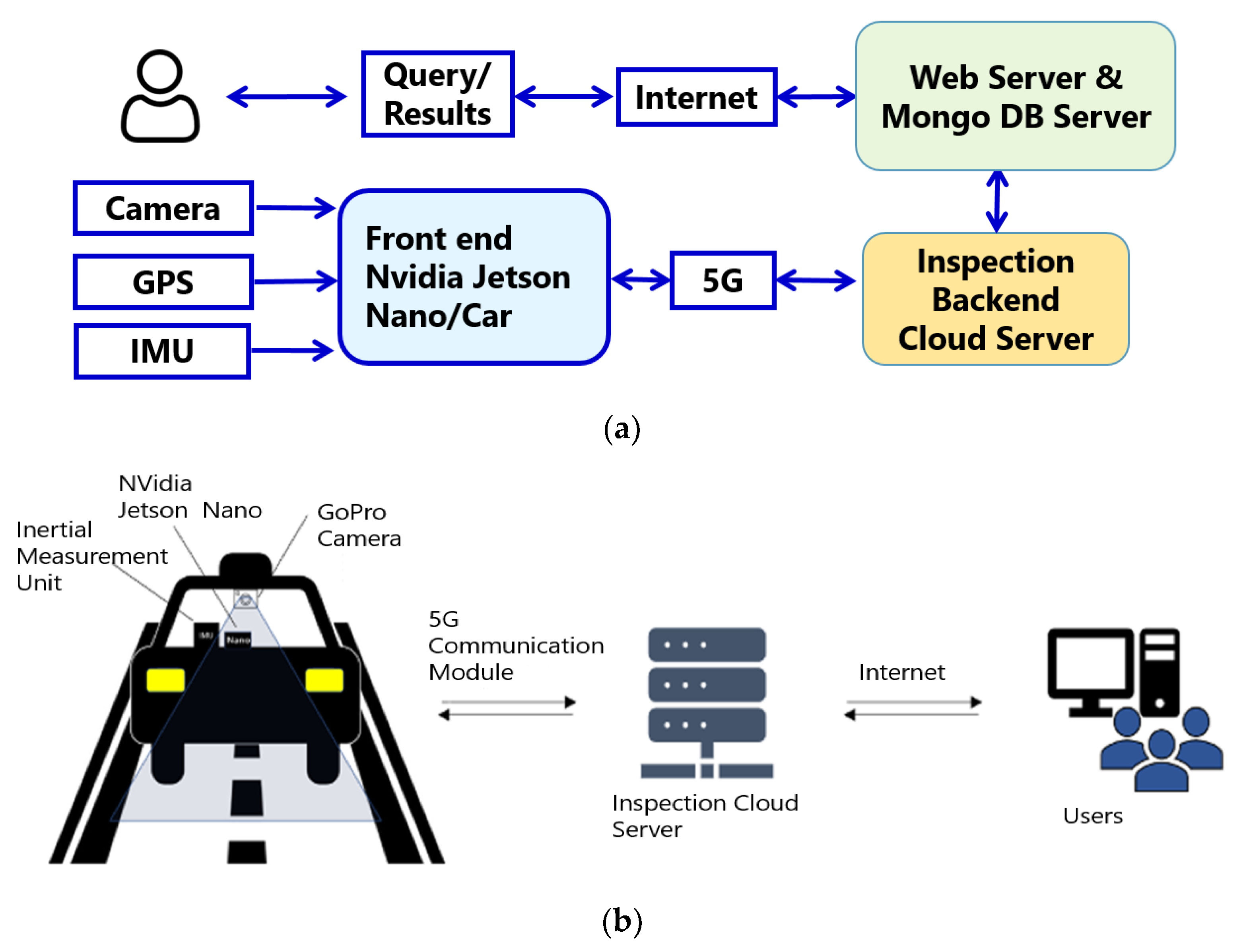
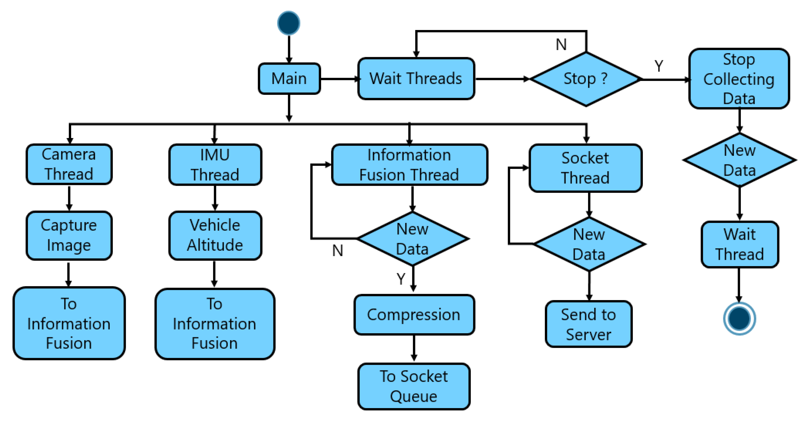
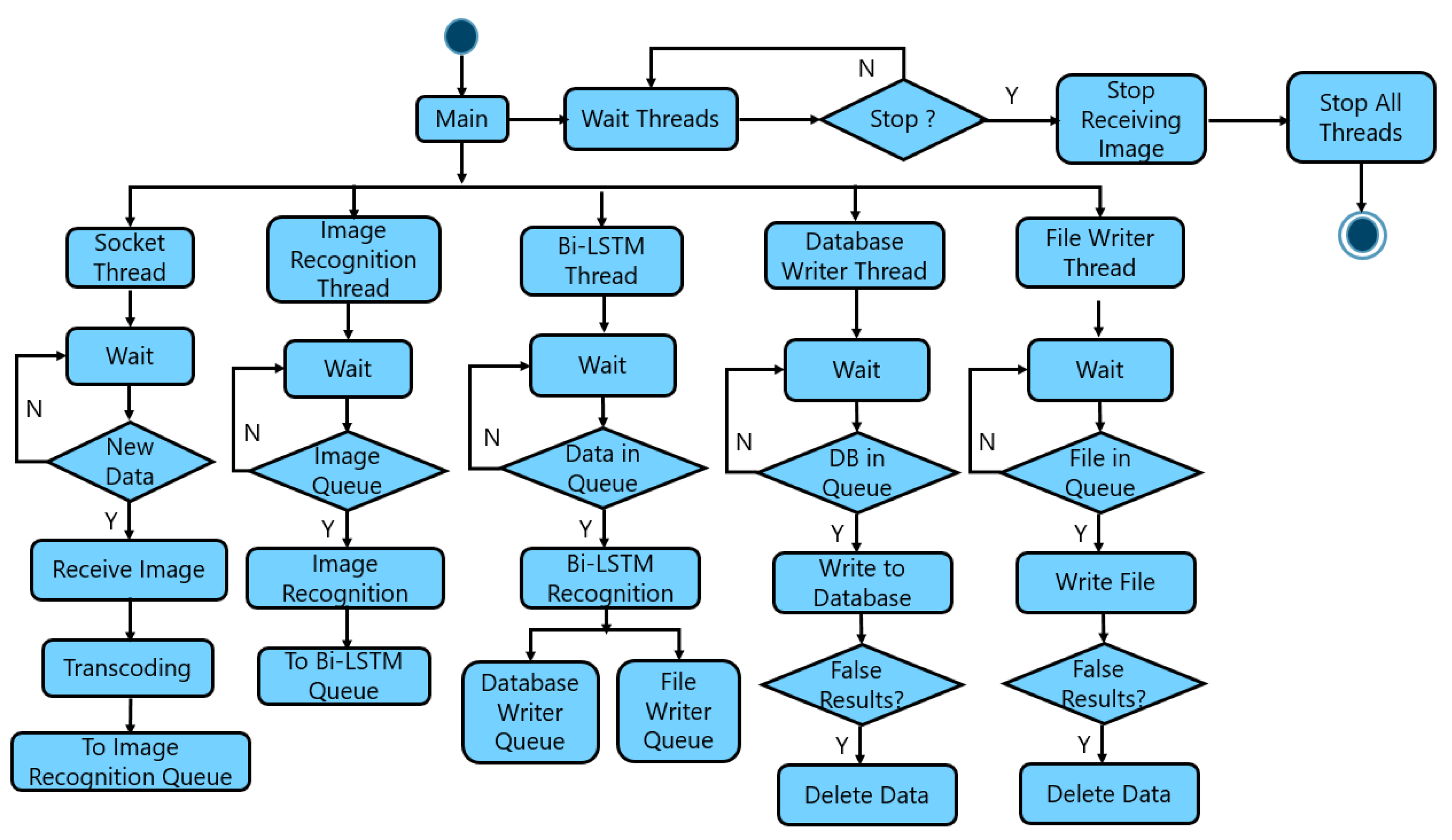
3.1. System Architecture
3.1.1. Road Pavement Defect Detection
3.1.2. GoPro Camera
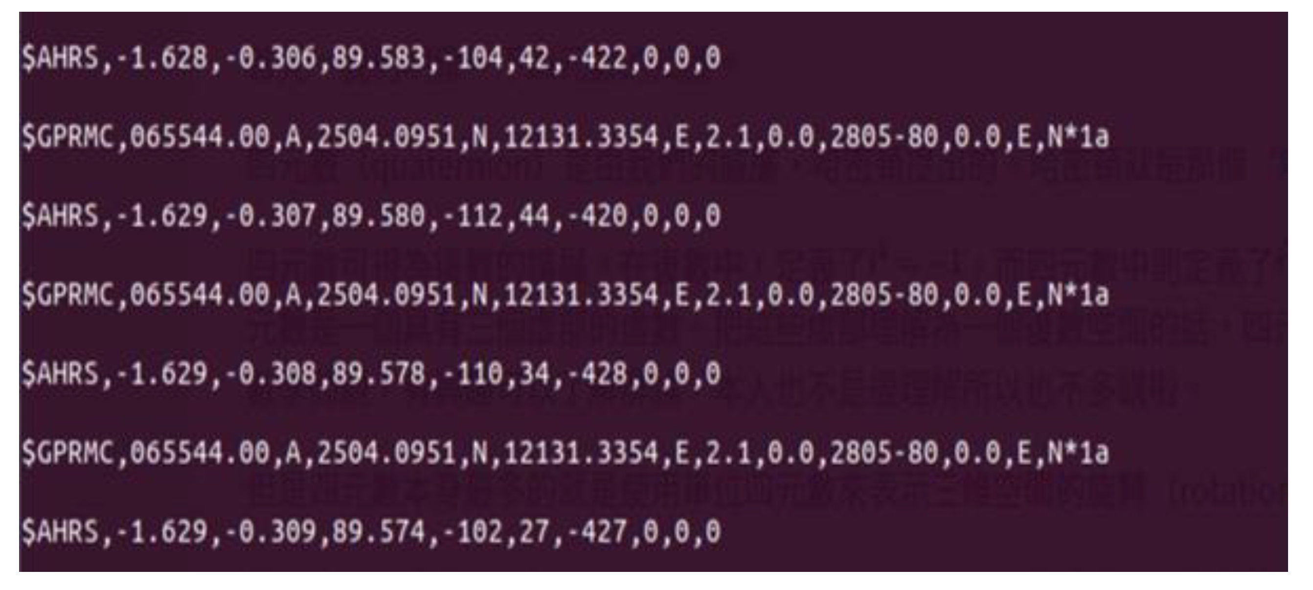
3.1.3. GPS and Inertial Measurement Unit
3.1.4. Nvidia Jetson Nano
3.1.5. Cloud Server
3.2. Dataset
3.2.1. Front View Image Dataset
3.2.2. Vehicle Vibration Dataset
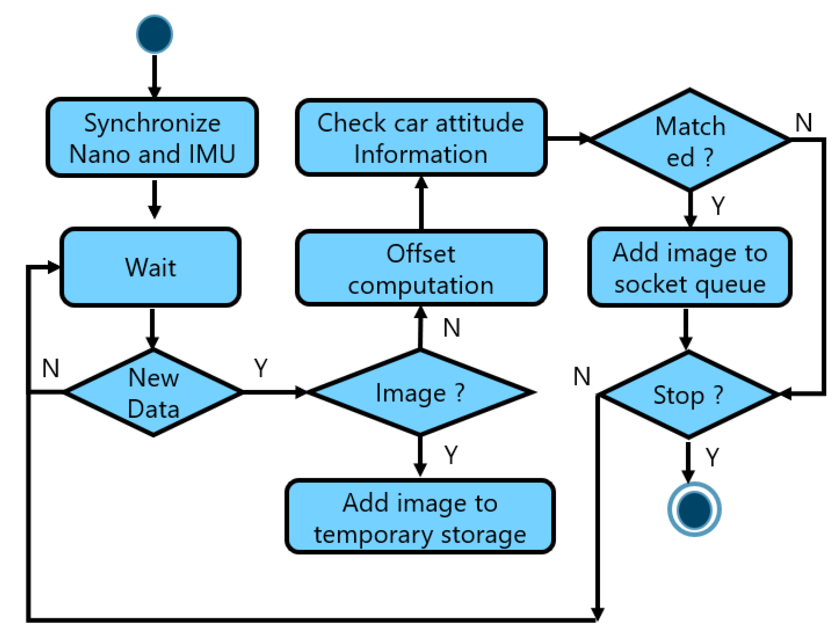
3.3. Integration of Visual and Vibration Information
4. Experimental Results and Analysis
4.1. Three-Axis Acceleration and Vehicle Attitude Analysis
4.1.1. Vehicle Information Pre-Processing
4.1.2. Vehicle Vibration Information Analysis
4.2. Visual Neural Network Training
4.3. One-Dimensional Neural Network Training
4.4. Field Test Results
4.5. Comparison with State-of-the-Art
5. Conclusions and Future Works
5.1. Conclusions
5.2. Future Works
Author Contributions
Funding
Informed Consent Statement
Data Availability Statement
Conflicts of Interest
References
- National Statistics, R.O.C. (Taiwan). Statistics on the Length of Roads in China in the Past Ten Years. 20 September 2022. Available online: https://statdb.dgbas.gov.tw/pxweb/Dialog/View.asp (accessed on 24 December 2022).
- Freeway Bureau, R.O.C. (Taiwan). Million Vehicle Kilometer Statistics. 13 December 2022. Available online: https://www.freeway.gov.tw/Publish.aspx?cnid=1656&p=26767 (accessed on 24 December 2022).
- Tamkang University. Pavement Engineering. 13 December 2022. Available online: https://mail.tku.edu.tw/yinghaur/lee/te/pdf (accessed on 24 December 2022).
- Zakeri, H.; Nejad, F.M.; Fahimifar, A. Image-Based Techniques for Crack Detection, Classification and Quantification in Asphalt Pavement: A Review. Arch. Computat. Methods Eng. 2017, 24, 935–977. [Google Scholar] [CrossRef]
- Kheradmandi, N.; Mehranfar, V. A Critical Review and Comparative Study on Image Segmentation-based Techniques for Pavement Crack Detection. Constr. Build. Mater. 2022, 321, 126162. [Google Scholar] [CrossRef]
- Gong, H.; Liu, L.; Liang, H.; Zhou, Y.; Cong, L. A State-of-the-Art Survey of Deep Learning Models for Automated Pavement Crack Segmentation. Int. J. Transp. Sci. Technol. 2024, 13, 44–57. [Google Scholar] [CrossRef]
- Qiu, J.Y. Research on Detection Based on Improved Mask RCNN Algorithms. Master’s Thesis, Department of Information and Communication Engineering, Chaoyang University, Taiwan, China, 2020. [Google Scholar]
- Wang, C.Y.; Bochkovskiy, A.; Liao, H.Y.M. YOLOv7: Trainable Bag-of-Freebies Sets New State-of-the-Art for Real-Time Object Detectors. In Proceedings of the 2023 IEEE/CVF Conference on Computer Vision and Pattern Recognition (CVPR), Vancouver, BC, Canada, 17–24 June 2023; pp. 7464–7475. [Google Scholar] [CrossRef]
- Gavilán, M.; Balcones, D.; Marcos, O.; Llorca, D.F.; Sotelo, M.A.; Parra, I.; Ocaña, M.; Aliseda, P.; Yarza, P.; Amírola, A. Adaptive Road Crack Detection System by Pavement Classification. Sensors 2011, 11, 9628–9657. [Google Scholar] [CrossRef] [PubMed]
- Her, S.-C.; Lin, S.-T. Non-Destructive Evaluation of Depth of Surface Cracks Using Ultrasonic Frequency Analysis. Sensors 2014, 14, 17146–17158. [Google Scholar] [CrossRef] [PubMed]
- Feng, H.; Li, W.; Luo, Z.; Chen, Y.; Fatholahi, S.N.; Cheng, M.; Wang, C.; Junior, J.M.; Li, J. GCN-Based Pavement Crack Detection Using Mobile LiDAR Point Clouds. IEEE Trans. Intell. Transp. Syst. 2022, 23, 11052–11061. [Google Scholar] [CrossRef]
- Aparna, Y.; Yukti, B.; Rachna, R.; Varun, G.; Naveen, A.; Aparna, A. Convolutional Neural Networks based Potholes Detection Using Thermal Imaging. J. King Saud Univ.-Comput. Inf. Sci. 2022, 34, 578–588. [Google Scholar] [CrossRef]
- Shenu, P.M.; Soumya, J. Automated Detection of Dry and Water-Filled Potholes Using Multimodal Sensing System. Doctoral Dissertation, Indian Institute of Technology Hyderabad, Kandi, Indian, 2012. [Google Scholar]
- Nienaber, S.; Booysen, M.; Kroon, R. Detecting Potholes Using Simple Image Processing Techniques and Real-World Footage. In Proceedings of the 34th Annual Southern African Transport Conference, Pretoria, South Africa, 6–9 July 2015. [Google Scholar]
- Varadharajan, S.; Jose, S.; Sharma, K.; Wander, L.; Mertz, C. Vision for Road Inspection. In Proceedings of the IEEE Winter Conference on Applications of Computer Vision, Steamboat Springs, CO, USA, 24–26 March 2014; pp. 115–122. [Google Scholar] [CrossRef]
- Achanta, R.; Shaji, A.; Smith, K.; Lucchi, A.; Fua, P.; Susstrunk, S. SLIC Superpixels; EPFL Technical Report 149300; EPFL: Lausanne, Switzerland, 2010. [Google Scholar]
- Ardeshir, N.; Sanford, C.; Hsu, D. Support Vector Machines and Linear Regression Coincide with Very High-Dimensional Features. Adv. Neural Inf. Process. Syst. 2021, 34, 4907–4918. [Google Scholar]
- Japan International Cooperation Agency. Pavement Inspection Guideline. Ministry of Transport, 13 December 2016. Available online: https://openjicareport.jica.go.jp/pdf/12286001_01.pdf (accessed on 24 December 2022).
- Redmon, J.; Farhadi, A. YOLOv3: An Incremental Improvement. arXiv 2018, arXiv:1804.02767. [Google Scholar]
- Bochkovskiy, A.; Wang, C.Y.; Liao, H.Y.M. YOLOv4: Optimal Speed and Accuracy of Object Detection. arXiv 2004, arXiv:2004.10934. [Google Scholar]
- Tan, M.; Pang, R.; Le, Q.V. EfficientDet: Scalable and Efficient Object Detection. In Proceedings of the 2020 IEEE/CVF Conference on Computer Vision and Pattern Recognition (CVPR), Seattle, WA, USA, 13–19 June 2020; pp. 10778–10787. [Google Scholar] [CrossRef]
- Li, C.; Li, L.; Jiang, H.; Weng, K.; Geng, Y.; Li, L.; Ke, Z.; Li, Q.; Cheng, M.; Nie, W.; et al. YOLOv6: A Single-Stage Object Detection Framework for Industrial Applications. arXiv 2022, arXiv:2209.02976. [Google Scholar]
- Liu, H.; Sun, F.; Gu, J.; Deng, L. SF-YOLOv5: A Lightweight Small Object Detection Algorithm Based on Improved Feature Fusion Mode. Sensors 2022, 22, 5817. [Google Scholar] [CrossRef] [PubMed]
- Ding, X.; Zhang, X.; Ma, N.; Han, J.; Ding, G.; Sun, J. RepVGG: Making VGG-style ConvNets Great again. In Proceedings of the 2021 IEEE/CVF Conference on Computer Vision and Pattern Recognition (CVPR), Nashville, TN, USA, 20–25 June 2021; pp. 13728–13737. [Google Scholar] [CrossRef]
- Carion, N.; Massa, F.; Synnaeve, G.; Usunier, N.; Kirillov, A.; Zagoruyko, S. End-to-End Object Detection with Transformers. arXiv 2020, arXiv:2005.12872. [Google Scholar]
- Wang, C.; Yeh, I.; Liao, H. You Only Learn One Representation: Unified Network for Multiple Tasks. J. Inf. Sci. Eng. 2021, 39, 691–709. [Google Scholar]
- Xu, S.; Wang, X.; Lv, W.; Chang, Q.; Cui, C.; Deng, K.; Wang, G.; Dang, Q.; Wei, S.; Du, Y.; et al. PP-YOLOE: An Evolved Version of YOLO. arXiv 2022, arXiv:2203.16250. [Google Scholar]
- Ge, Z.; Liu, S.; Wang, F.; Li, Z.; Sun, J. YOLOX: Exceeding YOLO Series in 2021. arXiv 2021, arXiv:2107.08430. [Google Scholar]
- Wang, C.; Bochkovskiy, A.; Liao, H.M. Scaled-YOLOv4: Scaling Cross Stage Partial Network. In Proceedings of the 2021 IEEE/CVF Conference on Computer Vision and Pattern Recognition (CVPR), Nashville, TN, USA, 20–25 June 2021; pp. 13024–13033. [Google Scholar]
- Ren, M.; Zhang, X.F.; Chen, X.; Zhou, B.; Feng, Z. YOLOv5s-M: A Deep Learning Network Model for Road Pavement Damage Detection from Urban Street-View Imagery. Int. J. Appl. Earth Obs. Geoinf. 2023, 120, 103335. [Google Scholar] [CrossRef]
- Zhou, Y.; Wei, Y.; Chen, J. Improved YOLOv4-Tiny Lightweight Country Road Pavement Damage Detection Algorithm. In Proceedings of the 2022 2nd International Conference on Algorithms, High-Performance Computing and Artificial Intelligence (AHPCAI), Guangzhou, China, 21–23 October 202; pp. 160–163. [CrossRef]
- Fassmeyer, P.; Kortmann, F.; Drews, P.; Funk, B. Towards a Camera-Based Road Damage Assessment and Detection for Autonomous Vehicles: Applying Scaled-YOLO and CVAE-WGAN. In Proceedings of the 2021 IEEE 94th Vehicular Technology Conference (VTC2021-Fall), Norman, OK, USA, 27–30 September 2021; IEEE: New York, NY, USA, 2021; pp. 1–7. [Google Scholar]
- Jeong, D. Road Damage Detection Using YOLO with Smartphone Images. In Proceedings of the 2020 IEEE International Conference on Big Data (Big Data), Atlanta, GA, USA, 10–13 December 2020; IEEE: New York, NY, USA, 2020; pp. 5559–5562. [Google Scholar]
- Yang, N.; Li, Y.; Ma, R. An Efficient Method for Detecting Asphalt Pavement Cracks and Sealed Cracks Based on a Deep Data-Driven Model. Appl. Sci. 2022, 12, 10089. [Google Scholar] [CrossRef]
- Sherstinsky, A. Fundamentals of Recurrent Neural Network (RNN) and Long Short-Term Memory (LSTM) Network. arXiv 2018, arXiv:1808.03314. [Google Scholar] [CrossRef]
- Staudemeyer, R.C.; Morris, E.R. Understanding LSTM—A Tutorial into Long Short-Term Memory Recurrent Neural Networks. arXiv 2019, arXiv:1909.09586. [Google Scholar]
- Schuster, A.M.; Paliwal, K.K. Bidirectional Recurrent Neural Networks. IEEE Trans. Signal Process. 1997, 45, 2673–2681. [Google Scholar] [CrossRef]
- Huang, Z.; Xu, W.; Yu, K. Bidirectional LSTM-CRF Models for Sequence Tagging. arXiv 2015, arXiv:1508.01991. [Google Scholar]
- goprotaiwancsl.com.tw. GoPro. Available online: https://www.goprotaiwancsl.com.tw/ (accessed on 24 December 2022).
- Newstar. Newstar AHRS Series Attitude and Heading Chip AH8. Available online: https://www.facebook.com/watch/?v=290400158530629 (accessed on 29 February 2024).
- Docs.novatel.com. GPRMC. 23 July 2023. Available online: https://docs.novatel.com/OEM7/Content/Logs/GPRMC.htm (accessed on 29 February 2024).
- Mathworks. Attitude and Heading Reference System. 2023. Available online: https://www.mathworks.com/help/nav/ref/ahrs.html (accessed on 29 February 2024).


| Field No. | Structure | Description |
|---|---|---|
| <1> | UTC | Hhmmss (hour, minute, second) |
| <2> | Position status | A = data valid, V = data invalid |
| <3> | Latitude | ddmm.mmmm (degree, minute) |
| <4> | Latitude direction | N = North, S = South |
| <5> | Longitude | ddmm.mmmm (degree, minute) |
| <6> | Longitude direction | E = East, W = West |
| <7> | Speed over ground, knots | 000.0~999.9 knots |
| <8> | Track made good, degrees | 000.0~359.9 degree |
| <9> | Date | ddmmyy (day, month, year) |
| <10> | Magnetic variation, degrees | 000.0~180.0 degree |
| <11> | Magnetic variation direction E/W | E (East) or W (West) |
| <12> | Positioning system mode indicator | A = autonomous, D = differential, E = estimated, N = data not valid |
| Field No. | Parameter | Format |
|---|---|---|
| <1><2><3> | x, y, z (Attitude) | xxx.xxx |
| <4><5><6> | x, y, z acceleration (GPS definition) | xxx.xxx |
| <7><8><9> | Angular rate | xxx.xxx |
| No. | Type | Sample Image | Definition |
|---|---|---|---|
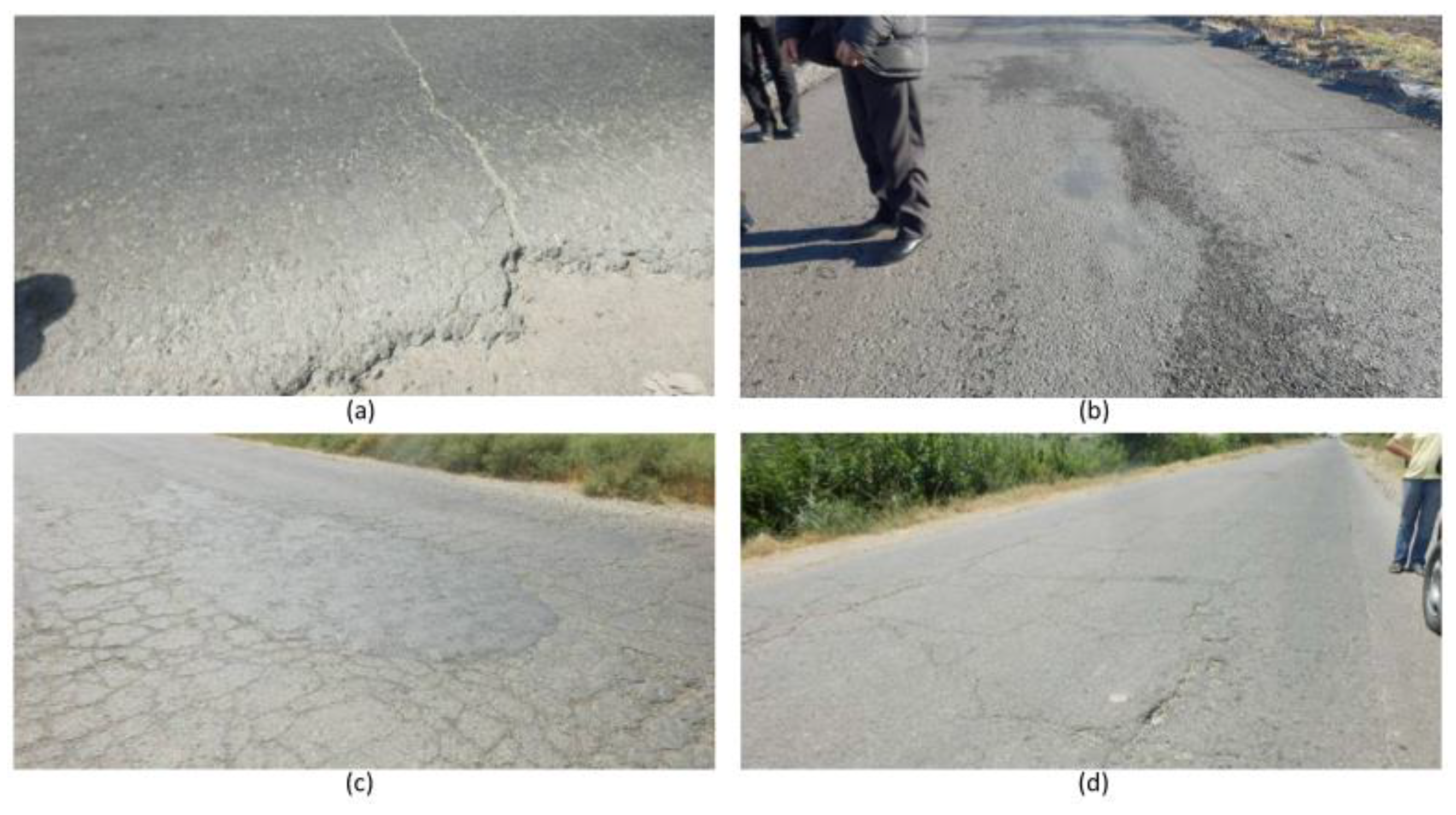
| 1 | Potholes |  | Visible potholes in road pavement |
| 2 | Cracks | 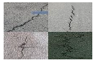 | Visible cracks in road pavement |
| No. | Type | Sample Image (Time Domain) | Definition (at Least Two Items Are Met) |
|---|---|---|---|
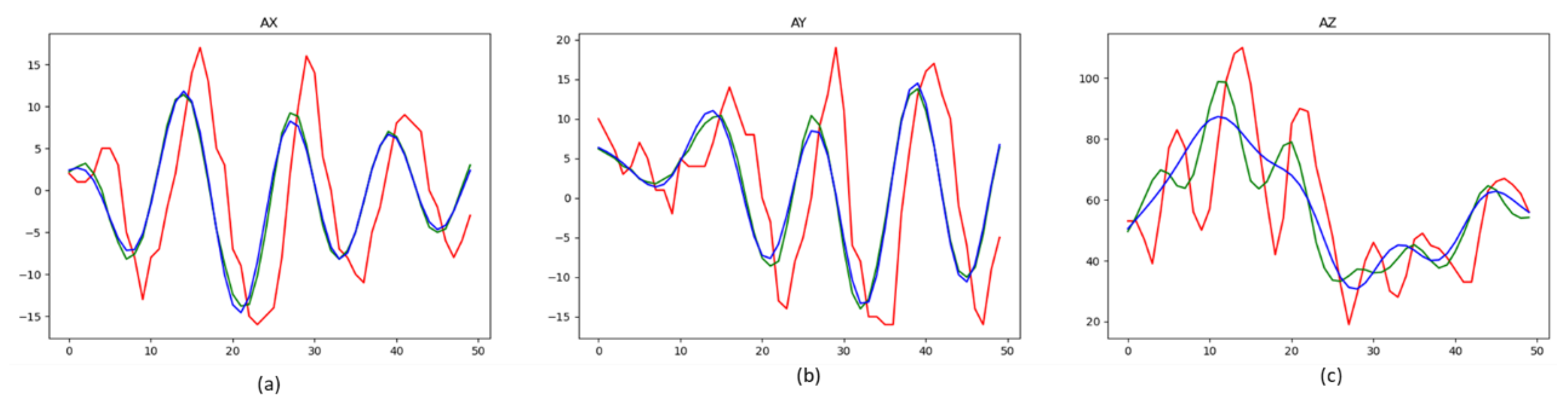
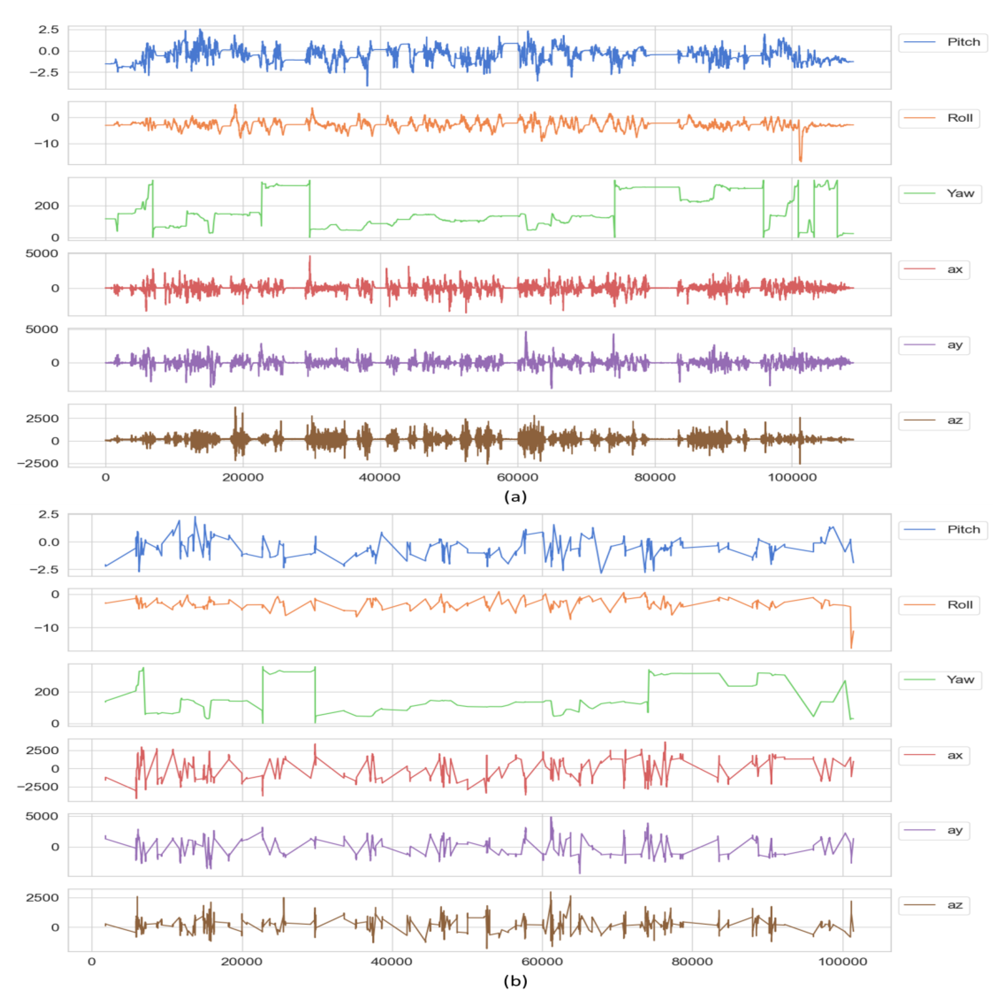
| 1 | Road pavement uneven—low risk | As shown in Figure 7a are the acceleration (ax, ay, az) in (x, y, z). |
|
| 2 | road pavement uneven—high-risk | As shown in Figure 7b are the acceleration (ax, ay, az) in (x, y, z). |
|
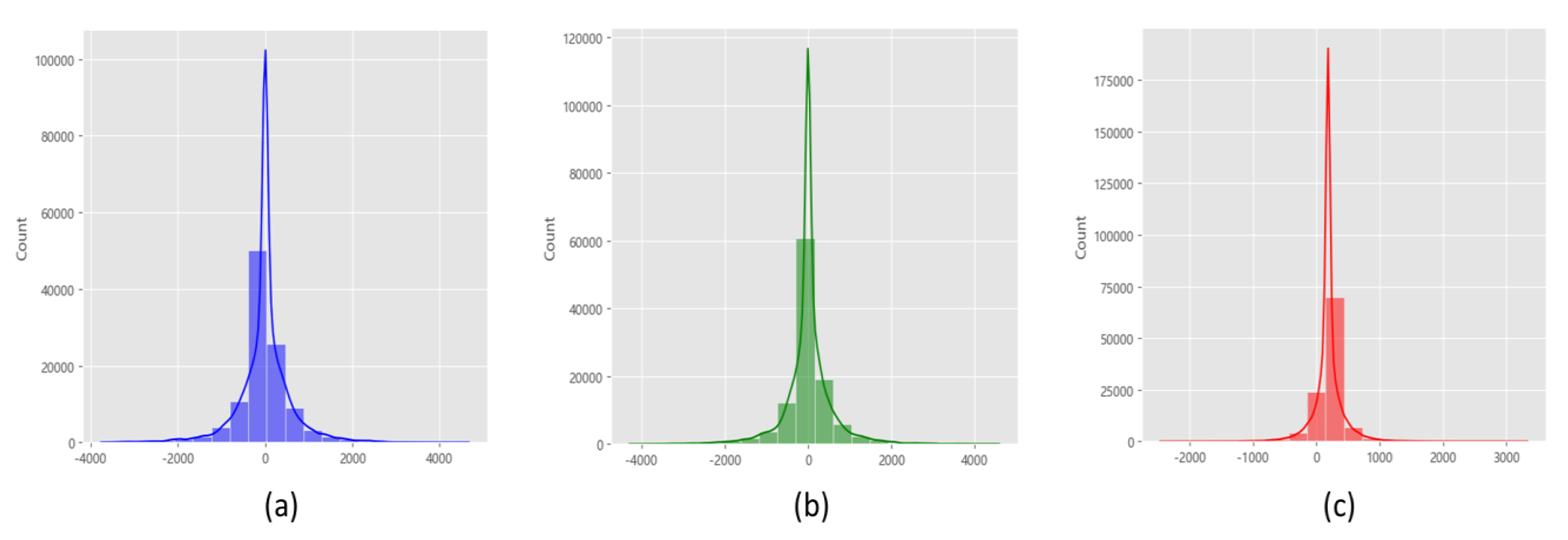
| Name | Std (mm/s2) |
|---|---|
| Ax | 603.58 |
| Ay | 584.28 |
| Az | 236.27 |
| Models | Precision | Recall | mAP | FPS |
|---|---|---|---|---|
| YOLOv4 | 87.6% | 88.6% | 89% | 20~22 |
| YOLOv4-tiny | 86.6% | 73.8% | 87% | 150~200 |
| YOLOR | 79.1% | 92.6% | 92.5% | 40~50 |
| YOLOv7 | 93.2% | 87.8% | 93.3% | 30~40 |
| TP | FP | FN | |
|---|---|---|---|
| Types\Models | v4/v4-tiny/R/v7 | v4/v4-tiny/R/v7 | v4/v4-tiny/R/v7 |
| Pothole | 47/50/50/45 | 7/3/14/0 | 5/2/2/7 |
| Crack | 31/15/32/32 | 4/7/8/5 | 5/21/4/4 |
| Metrics | Precision | Recall | Accuracy | FPS |
|---|---|---|---|---|
| Types\Models | RNN/LSTM/Bi-LSTM | RNN/LSTM/Bi-LSTM | RNN/LSTM/Bi-LSTM | RNN/LSTM/Bi-LSTM |
| Pavement uneven—low risk | 99%/98.6%/99.1% | 99.3%/99.4%/99.6% | 98.9%/98.1%/98.7% | |
| Pavement uneven—high risk | 77.2%/71.4%/80.4% | 82.9%/85.3%/90.2% | 66.6%/63.6%/74% | |
| Average | 88.1%/85%/89.75% | 91.1%/92.35%/94.9% | 82.75%/80.85%/86.35% | 25/33.3/40 |
| TP | FP | FN | |
|---|---|---|---|
| Types\Models | RNN/LSTM/Bi-LSTM | RNN/LSTM/Bi-LSTM | RNN/LSTM/Bi-LSTM |
| Pavement uneven-low risk | 1039/1034/1040 | 7/6/4 | 10/14/9 |
| Pavement uneven-high risk | 34/35/37 | 10/14/9 | 7/6/4 |
| Recall | Precision | ||
|---|---|---|---|
| Pavement image | Pothole | 95.0% | 92.8% |
| Crack | 92.5% | 91.9% | |
| Vehicle attitude | Uneven—low risk | 99.4% | 99.1% |
| Uneven—high risk | 93.0% | 82.3% | |
| Integrated detection | Pothole—high risk | 94.4% | 91.9% |
| Crack—high risk | 86.0% | 75.6% |
| Items | Sensors | Precision/Recall | Classification | Defect Types | FPS |
|---|---|---|---|---|---|
| [9] | Line Camera | 98.29%/93.86% | SVM | Ten types | NA |
| [10] | Ultrasonic | Error < 7% | FFT | Crack depth | NA |
| [11] | LiDAR | 70%/73.9% | GCN | Crack | NA |
| [12] | Thermal imaging | Accuracy 97.08% | CNN-ResNet | Pothole | NA |
| [31] | Smartphone | 65%/55% | YOLO4 Tiny | Four types of cracks | NA |
| [32] | Smartphone | F1 score = 51.9% | Scaled YOLOv4 | Four types of cracks | 73.8 |
| [33] | Smartphone | F1 score = 58.4% | YOLOv5x | Four types of cracks | 33.3 |
| [34] | CCD+LED | 83.38%/90.45% | YOLOv5s | Cracks/sealed cracks | 67.5 |
| [30] | CCD | 78.2%/72.1% | YOLOv5s-M | Seven types | 42 |
| Ours | Camera +IMU | 93.3%/86.35% | YOLOv7+Bi-LSTM | Pothole/crack | >30 |
Disclaimer/Publisher’s Note: The statements, opinions and data contained in all publications are solely those of the individual author(s) and contributor(s) and not of MDPI and/or the editor(s). MDPI and/or the editor(s) disclaim responsibility for any injury to people or property resulting from any ideas, methods, instructions or products referred to in the content. |
© 2024 by the authors. Licensee MDPI, Basel, Switzerland. This article is an open access article distributed under the terms and conditions of the Creative Commons Attribution (CC BY) license (https://creativecommons.org/licenses/by/4.0/).
Share and Cite
Hsieh, C.-C.; Jia, H.-W.; Huang, W.-H.; Hsih, M.-H. Deep Learning-Based Road Pavement Inspection by Integrating Visual Information and IMU. Information 2024, 15, 239. https://doi.org/10.3390/info15040239
Hsieh C-C, Jia H-W, Huang W-H, Hsih M-H. Deep Learning-Based Road Pavement Inspection by Integrating Visual Information and IMU. Information. 2024; 15(4):239. https://doi.org/10.3390/info15040239
Chicago/Turabian StyleHsieh, Chen-Chiung, Han-Wen Jia, Wei-Hsin Huang, and Mei-Hua Hsih. 2024. "Deep Learning-Based Road Pavement Inspection by Integrating Visual Information and IMU" Information 15, no. 4: 239. https://doi.org/10.3390/info15040239
APA StyleHsieh, C.-C., Jia, H.-W., Huang, W.-H., & Hsih, M.-H. (2024). Deep Learning-Based Road Pavement Inspection by Integrating Visual Information and IMU. Information, 15(4), 239. https://doi.org/10.3390/info15040239