Intuitionistic Fuzzy Sets for Spatial and Temporal Data Intervals

Abstract

Spatial and temporal uncertainties are found in data for many critical applications. This paper describes the use of interval-based representations of some spatial and temporal information. Uncertainties in the information can arise from multiple sources in which degrees of support and non-support occur in evaluations. This motivates the use of intuitionistic fuzzy sets to permit the use of the positive and negative memberships to capture these uncertainties. The interval representations will include both simple and complex or nested intervals. The relationships between intervals such as overlapping, containing, etc. are then developed for both the simple and complex intervals. Such relationships are required to support the aggregation approaches of the interval information. Both averaging and merging approaches to interval aggregation are then developed. Furthermore, potential techniques for the associated aggregation of the interval intuitionistic fuzzy memberships are provided. A motivating example of maritime depth data required for safe navigation is used to illustrate the approach. Finally, some potential future developments are discussed.

1. Introduction

Spatial and temporal uncertainties commonly occur in a variety of problems. The motivations of this research are found in many areas in which there is uncertainty in temporal and spatial data. The contributions of this paper are to introduce interval-based representations of spatial and temporal information. Next, fuzzy intuitionistic memberships are used to represent the subjective uncertainty for such intervals. The interval representations introduced comprise both simple and complex or nested intervals, and the relationships between both sorts of intervals are illustrated. Finally, averaging and merging approaches to aggregations of intervals and interval intuitionistic fuzzy memberships are developed.

Some typical examples are found in applications including the spatial and temporal aspects that arise during intelligence analysis and prediction [1], in the area of criminal forensics [2,3,4], and in forensic criminal anthropology [5]. Consider the case of a suspicious death. A body may be found in another location in which the crime did not occur. Then, there may be a number of uncertain indicators as to where death actually happened. Also, based on an environmental issue such as temperature, the medical examiner can provide a probable time range for the death, but also allow uncertainty of a wider time interval and a degree of confidence related to this. Relationships between the intervals can help lead to resolution of a crime, as overlap between the probable times and locations for a suspect could be significant evidence in the investigation [6].

A well-known example of the impact of these sorts of imprecisions can be found in the search for Malaysia Airlines Flight 370. The flight disappeared over the Indian Ocean in 2014 and there was notable uncertainty in the times and the location of its possible flight path. Information about the flight came from various sources with multiple uncertainties including radar fixes, fuel capacity, plane characteristics, etc. [7]. A better specification of the temporal intervals of the flight time and spatial intervals of the flight path could have provided significant time and expense improvements for the search.

For this sort of spatial and temporal information, specifically interval-based information for this research, much of the uncertainty commonly occurs with investigators and experts giving opinions both supporting and not supporting information in different degrees. It is specifically because of these typical evaluations that intuitionistic fuzzy memberships of spatial and temporal intervals are used in this paper to capture these sorts of situations.

In this paper, Section 2 presents relevant spatial and temporal research and then the techniques used for interval representation and fuzzy intuitionistic sets. Then, in Section 3, simple and complex intervals are introduced and the relationships between such intervals are provided. Next, the approach to aggregation of both intervals and fuzzy intuitionistic memberships is developed. An example application of water depth data intervals as required for maritime navigation is discussed. A sample computation of aggregations of such data is performed and evaluations discussed. Lastly, in Section 4, the main contributions of the paper are summarized and possible new research directions are described.

2. Methods and Materials

2.1. Relevant Background

In this section, previous relevant research in the areas of both temporal and spatial information is reviewed.

2.1.1. Temporal Information Research

One approach [8] considers a combination of inconsistent temporal interval relations and probabilistic uncertainty conditions. The semantics of such relations can be conflicting, and this is the basis of the concept of inconsistent relations developed in this approach to deal with the uncertainty and conflict for temporal information. Another development used an interval approach based on semi-intervals [9]. Here, conceptual neighborhoods were utilized so that temporal relationships dealing with coarse and incomplete knowledge could be resolved. These previous approaches do not deal directly with temporal intervals, but instead consider the uncertainty relationships between such intervals. For the development of temporal databases [10], the basic constructs of time-related information are modeled by the types, point, interval, and span [11]. Another approach directly addresses fuzzy temporal intervals [12,13]. In particular, using a trapezoidal fuzzy interval, expressions are designed for the temporal relationships as well as inferencing for this representation of intervals. Interval temporal logics have been based on the fuzzy Halpern theory for use in several areas [14]. Applications of fuzzy temporal approaches include scheduling and sequence modeling and evaluations of equipment effectiveness [15,16]. Often, spatial and temporal data are combined in fuzzy spatiotemporal models. These arise from integrating multisource data [17] and from data modeled by UML [18]. Additionally, rough set techniques have been used in the development of temporal information systems [19,20].

2.1.2. Spatial Information Research

For spatial information, the issues of dealing with its imprecision and uncertainty aspects have been considered by many researchers [21,22]. These issues arise especially in the implementation and usage of geographical information systems (GISs) [23]. When employing geographical information systems, in many applications, the value of decisions using such tools will largely depend on decision makers’ ability to assess the validity and reliability of the information as the basis for their decisions [24,25]. Several approaches have been developed for manipulation and querying of fuzzy data in image processing [26,27,28], including the R software package. Additionally, fuzzy spatial object models and inferences have been used in some image processing approaches [29,30]. An application to environmental planning used a fuzzy spatial situational assessment of wildfires [31].

In order to make effective use of geographical information systems technology, the user has to be able to judge the characteristics of error and their degree in spatial databases, follow any error during GIS operations, and finally provide estimates of the accuracy of the results which may be both graphic and numeric. The broad term accuracy is typically used to represent the various types and characteristics of potential errors in geographical information systems. However, for our purposes in this paper the typical aspects that can be addressed by one or more of the various soft computing techniques are considered. Often, the operations and processes used for spatial data make the assumption that the common attributes and features, as well as their relationships, have a priori been developed exactly and precisely. This ignores the fact that imprecision and inexactness occur for the location of features and the specification of attribute values. Such imprecision and inexactness can be produced in the processes found in several stages of the compilation of data and development of a database. Spatial data uncertainty modeling has utilized a variety of techniques including concepts from non-monotonic logics, Dempster–Shafer evidence theory, fuzzy sets such as type 2 fuzzy and intuitionistic fuzzy sets, and rough set theory approaches [32,33,34]. Dempster–Shafer approaches have been used to deal with uncertainty in both spatial [35] and temporal data [36]. For both of these, a nested interval representation used an inner interval that was more certain and an outer interval that was possible but less certain.

2.2. Fuzzy Set Theory

This section first provides details on the formal mathematical background to be applied. This includes basic definitions of fuzzy sets, intuitionistic fuzzy sets, and interval theory.

2.2.1. Fuzzy Sets

Fuzzy set representations [37,38] are used to provide degrees of membership in a set for data values in contrast to crisp sets. For a domain D, a fuzzy set, FS, is

FS(D) = {<a_j, m(a_j)>|0 ≤ m(a_j) ≤ 1}, where a_j ∈ D, j = 1 to n

Here, m(a_j) is the membership of the data value a_j.

2.2.2. Intuitionistic Fuzzy Sets

By allowing negative as well as positive memberships to be specified, intuitionistic fuzzy set theory represents an extension of ordinary fuzzy set theory. Recall that an ordinary fuzzy set has only one membership value for a data element a_i. An intuitionistic fuzzy set IFS(D) [39] permits positive, m_S(a_i), as well as negative membership values, m_S * (a_i).

IFS(D) = {<a_i, m(a_i), m * (a_i)>|a_i ∈D} where m(a_i), m * (a_i), ∈ [0, 1].

Specifically, the sum of the membership, m(a_i), and non-membership, m * (a_i), is not necessarily one: 0 ≤ m(a_i) + m * (a_i) ≤ 1. Additionally, the hesitation h (a_i)

h(a_i) = 1 − (m(a_i) + m * (a_i))

is the degree of indeterminacy (hesitation).

Extensions to fuzzy intuitionistic sets are the Pythagorean [40] and the Fermatean [41] approaches. They each provide extensions to the membership value restrictions, which are, respectively,

0 ≤ m(a_i)² + m * (a_i)² ≤ 1

0 ≤ m(a_i)³ + m * (a_i)³ ≤ 1

This simply allows fewer restrictions for an individual to express their opinions regarding memberships. This can be useful as the psychological aspect of providing both positive and negative evaluations can be difficult. For example, consider a case for memberships specified as

m(a_i) = 0.85; m * (a_i) = 0.65 and then m(a_i) + m * (a_i) = 1.5 > 1

Now consider what these constraints are for Pythagorean and Fermatean approaches, respectively:

0.72 + 0.42 = 1.14 > 1 and 0.62 + 0.27 = 0.89 < 1.

So, in a Fermatean representation, the less restricted memberships are allowed.

2.2.3. Interval Representation

In representing interval-valued uncertainty with fuzzy sets as opposed to the ordinary crisp set representations, an overview of approaches to the representation of intervals is provided. Here, the formalisms for intervals and interval arithmetic [42,43] are introduced. Letting D be the domain, intervals can then be represented by the values of the upper, z^†, and lower, z_†, bounds of an interval I (z):

I (z) = [z_†, z^†] = {z ∈ D|z_† ≤ z ≤ z^†}

where z_† and z^† are a pair of values from D.

For an interval I (z), the size or width of the interval, IW, is given as the difference of the lower and upper bounds:

IW: I (z) → R⁺; IW (I (z)) = |z_† − z^†|

The interval width can be utilized as an information metric of the uncertainty for the IFS of a data value z [44].

For intervals, many operations including arithmetic valuations have been defined in general; however, for this paper, it is necessary to only utilize addition and subtraction. So, the resultant intervals for addition or subtraction operations are shown next:

[z_†, z^†] OP [w_†, w^†] = [(z_† + w_†), (z^† + w^†)] or [(z_† − w_†), (z^† − w^†)]

where w ∈ Z, w_† ≤ w ≤ w^†.

Another operation that can be applicable for some applications is the idea of merging intervals. Using Min on the lower bounds of intervals and Max on the upper bounds, the merger of two intervals is then

Merge([z_†, z^†], [w_†, w^†]) = [Min (z_†, w_†), Max (z^†, w^†)]

Also, a definition of a subset for intervals is

[z_†, z^†], ⊆ [w_†, w^†] iff (z_† ≤ w_†) ∧ (z^† ≤ w^†).

3. Results

In this section, the approach to interval representation using both simple and complex or nested intervals is considered. The intervals’ relationships will be outlined and illustrated. Next, the aggregations of the uncertain intervals are provided. The averaging and merging of both simple and complex intervals are described. Then, the final step is the combination of the interval aggregations with the aggregation of the fuzzy memberships using effective decision-making criteria.

Uncertain spatial or temporal intervals will be represented with the data interval component denoted as S_i and the associated intuitionistic memberships denoted as Mb(S_i) = (m(S_i), m * (S_i)). So, finally, a data collection D = {D₁, … D_p} is

D = {D₁ = (S₁, Mb(S₁)), D₂ = (S₂, Mb(S₂ )), … D_p = (S_p, Mb(S_p))}.

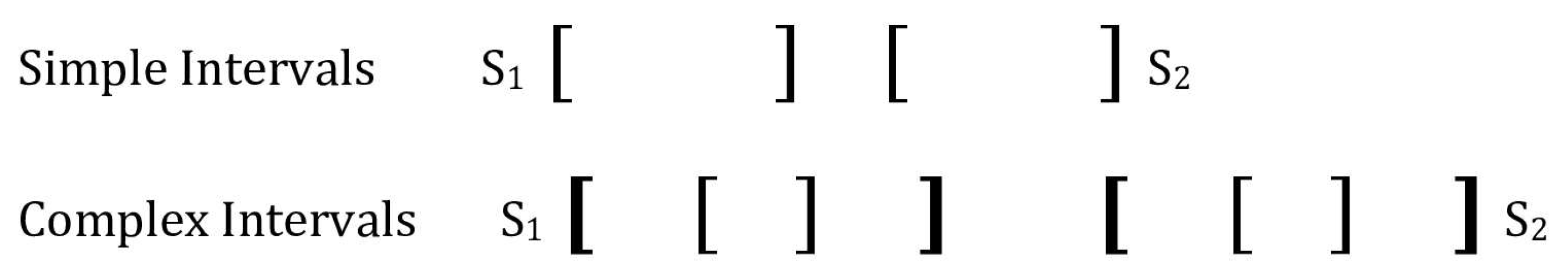
3.1. Simple and Complex Intervals

Intervals will consist of two sorts: simple and complex. A simple interval is just one for which the endpoints are well known as needed for an application:

S_i = [Sl_i, Sh_i]

Now, a complex interval representation is one in which a pair of nested intervals, IS_i and OS_i, is used. The inner interval IS_i represents the more certain data range and correspondingly the outer interval OS_i provides a plausible but less certain range:

IS_i = [ISl_i, ISh_i], OS_i = [OSl_i, OSh_i ] where OSl_i ≤ ISl_i and OSh_i ≥ ISh_i

For example:

S_i = [OS_i = [50, 100]; IS_i = [60, 80]]

In general, the complex interval arises when, based on the initial uncertainty of information sources, the information is developed as nested intervals of more certain sub-intervals inside of the information range of values that are also possible.

Now, in general, for either simple or complex intervals there is the associated fuzzy intuitionistic membership associated with an interval. These sorts of memberships are typically generated by evaluations of the temporal or spatial information by experts or analysts. They may be judging based on assessments of the source of the information, using either direct field or sensor-acquired measurements. Their judgments on the information are reflected in their assignment of positive and negative degrees of fuzzy memberships. These assessments are associated with the data in either simple or the already described complex intervals. Another finer assessment that may be made is when separate memberships are associated with both the inner and outer nested intervals.

3.2. Interval Relationships

For aggregation of intervals, either an averaging aggregation or a merging aggregation can be used. Both of these must take into account the following possible relationships between intervals:

Non-intersecting, NI, abutting, AB, overlapping, OV, but not contained, and contained, CO, but not equal as a special case.

The specifications for these relations for two simple intervals S₁ and S₂ need to be provided before considering the case of nested intervals. For nested intervals, relationships can be considered as between outer and inner intervals, and not all of the potential cases but just some representative cases are shown. Also, it is feasible to consider the relationship between a simple and a complex interval. In all cases, the relationship of intervals is considered as moving from left to right on the x-axis.

• Non-intersecting: NI(S₁, S₂)

The intervals are disjointed, S₁ ∩ S₂ = ∅, and there are conditions for both simple and complex intervals that are required.

• Simple interval: Sh₁ < Sl₂
• Complex interval: OSh₁ < OSl₂

These conditions are shown in Figure 1 for simple and complex intervals.

Additionally, a numeric example illustrating complex intervals is

S₁ = [50 [60, 80] 100]; S₂ = [150 [160, 180] 200]

A consideration for the case of non-intersecting intervals could occur for some aggregations. If a restriction on aggregations is assumed so that values not appearing in one or more of the original intervals should appear in the result, then it may be violated for intervals in this case. Considering the numeric example, if the value 120 would result for an S₁ and S₂ aggregation, this might be considered as an invalid result.

2.

Abutting: AB (S₁, S₂)

For abutting, the condition that applies is between the upper bounds of S₁ and lower bounds of S₂. The specific conditions for simple and complex intervals are

• Simple interval: Sh₁ = Sl₂
• Simple to complex: Sh₁ = OSl₂
• Complex interval: OSh₁ = OSl₂

For example, for complex intervals,

S₁ = [50 [60, 80] 100]]; S₂ = [100 [160, 180] 200]]

3.

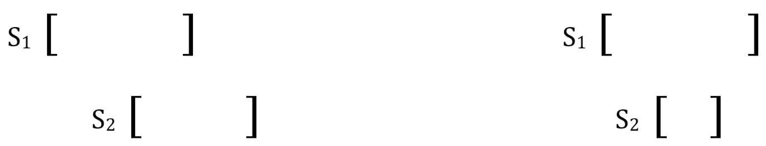
Overlapping: OV(S₁, S₂)

In general, this means that the intersection of intervals is non-empty; S₁ ∩ S₂ ≠ ∅. Next, it may be of interest to consider overlapping with outer or inner intervals for simple with complex intervals and complex intervals with complex intervals. Here are some example cases that include overlapping but not containing conditions.

Simple interval:

• Sh₁ > Sl₂; Example on the left side of Figure 2.
• For example, S₁ = [1305, 1345], S₂ = [1340, 1420]

Simple to complex:

• Case 1. Outer overlap only: Sh₁ > OSl₂ and Sh₁ ≤ ISl₂
• For example, S₁ =[50, 100]; S₂ = [90 [160, 180] 200]
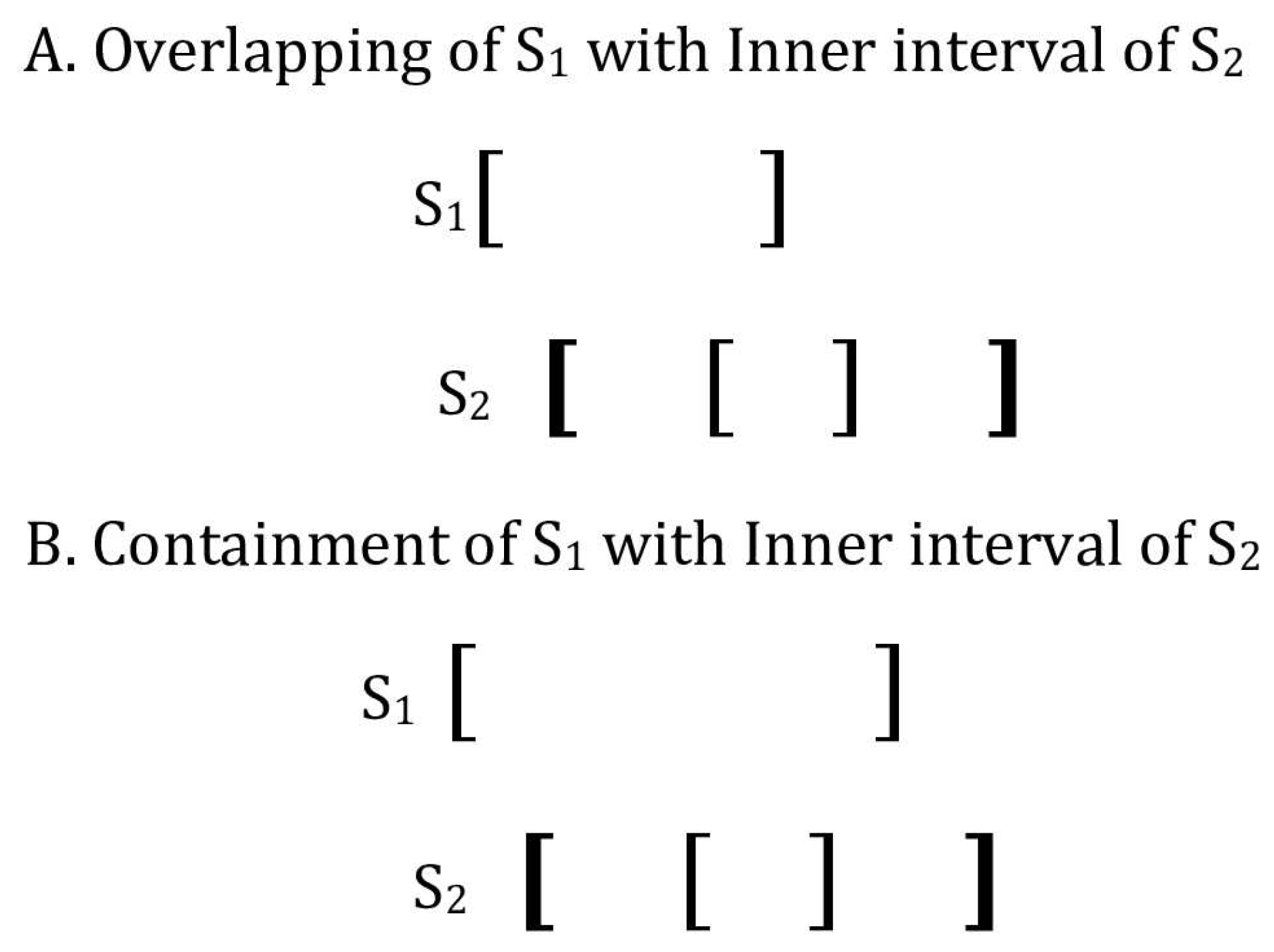
• Case 2. Figure 2A. Inner overlap but not contained: Sh₁ > ISl₂
• and Sh₁ ≤ ISh₂

Complex to complex:

In general, only some of the possible cases need to be considered:

• Outer interval overlap: OSh₁ > OSl₂
• Outer–inner interval overlap: OSh₁ > ISl₂

4.

Contained: CO(S₁, S₂)

Simple intervals:

• S₂ contained in S₁: Sl₂ > Sl₁ and Sh₂ < Sh₁. Therefore, note that if the intervals satisfy the containing condition this means an overlap condition is also implied. The right side of Figure 3 illustrates this.
• For example, S₁ = [1340, 1420], S₂ = [1345, 1400]

Simple to complex:

• Inner interval of S₂ contained in S₁ (Figure 2B):
• S₁₁ < ISl₂ and Sh₁ > ISh₂

A. Overlapping of S₁ with inner interval of S₂

3.3. Interval Aggregation

Two approaches can be used for interval aggregation, AGG(S_i, S_k): averaging, AV, and merging, MG. Each must be adapted for use with complex as well as simple intervals.

3.3.1. Simple Intervals

Here, first consider simple intervals. For averaging and merging, the interval endpoints are used to produce the interval AGG(S_i, S_k), denoted AS_ik or MS_ik, respectively:

AS_ik = AV(S_i, S_k) = [(Sl_i + Sl_k)/2, (Sh_i + Sh_k)/2]

MS_ik = MG(S_i, S_k) = [Min(Sl_i, Sl_k), Max(Sh_i, Sh_k)]

For both of these, if the intervals have a non-intersecting relationship, a possibly invalid value can occur in the result. Also, consider the width of the intervals, IW, as one indicator of the uncertainty of intervals. For averaging aggregation, the width of IW(AS_ik) is less than or equal to the maximum of the two original intervals IW(S_i) and IW(S_k). For MG (S_i, S_k), the resultant interval width IW(MS_ik) will always be greater than that of the averaging aggregation IW(AS_ik) [45].

3.3.2. Complex Intervals

Now, a similar approach can be followed for complex intervals by averaging the inner and outer interval endpoints. So here, for the inner interval, the following is true:

AVI(S_i, S_k) = [ISl_ik = (ISl_i + ISl_k)/2, ISh_ik = (ISh_i + ISh_k)/2]

Then, obtaining for the outer intervals, AVO(S_i, S_k), similarly, the complex interval result finally obtained by nesting AVI(S_i, S_k) and AVO(S_i, S_k) is

AS_ik = AV(S_i, S_k) = [OSl_ik [ISl_ik, ISlh_ik] OSlh_ik]

Likewise, following up with the merging of the intervals, first, for the inner interval, there is

MGI(S_i, S_k) = [ISl_ik = Min (ISl_i, ISl_k), ISh_ik = Max(ISh_i, ISh_k)]

So following this operation on the outer interval, the final merged interval is obtained:

MS_ik = MG(S_i, S_k) = [OSl_ik [ISl_ik, ISh_ik] OSh_ik]

For both of these aggregations, it must be determined if the final aggregated result is valid. This means the nesting of the inner interval inside of the outer interval is correctly maintained. If the original intervals, S_i, S_k, are correctly nested, the contained relationship, CO(OS_i, IS_i), holds. Then, this means ISl_i = OSl_i + n, n ≥ 0. Likewise, ISl_k = Osl_k + m, m ≥ 0. Then,

ISl_ik = (ISl_i + ISl_k)/2 = (OSl_i + n, OSl_k + m)/2 = OSl_ik + (n + m)/2, (n + m)/2 ≥ 0

The same analysis can be performed for the upper endpoints of the intervals, and then CO(OS_ik, IS_ik) satisfies the contained relationship.

Next, the nesting is seen to be maintained when the aggregation is merging.

ISl_ik = Min (ISl_i, ISl_k) = Min (OSl_i + n, OSl_k + m)

Let (OSl_i + n) ≥ (OSl_k +m), and so ISl_ik = OSl_i + n, n ≥ 0, which is a valid nesting. Again, the same applies to the upper bound, and so CO (OS_ik, IS_ik) satisfies the contained relationship.

Now, when considering comparisons of merging and averaging aggregation, it is clear that merging results entail more uncertainty. Still, for applications where the original values of intervals should be preserved, merging aggregation should be considered. This is because the intervals produced by averaging are often less reflective of the information in the original intervals. Intuitively, this illustrates the contrasting optimistic (averaging) versus pessimistic (merging) interpretations.

3.3.3. Aggregation of Memberships

Following the aggregation of intervals, the aggregation of the associated memberships, AGG(Mb_i, Mb_k), is addressed. Afterwards, both interval and membership aggregations are combined to provide a final result. For AGG(Mb_i, Mb_k), a straightforward approach uses a possible set of operators, {Min, Max, Avg), which are generally seen as good default choices [46,47]. Some alternatives may be used to provide aggregation that addresses problems with the standard set in certain circumstances, such as an OWA averaging approach [48]. For the purposes of this paper, the simpler approach is used as it is sufficient to illustrate the overall intent. The choices of Max versus Min represent an aggressive versus a more conservative stance. In case there is no preference, an Average is reasonable. So, for positive and negative memberships the aggregation is

AGG(Mb₁, …Mb_p ) = (OP_i-1..p (m (S_i)), OP_i-1..p (m * (S_i)))

where the operator OP is either Min, Max, or Avg. So for each, there are the following:

m_Min = Min_{i = 1..p} m (S_i)    m * _Min = Min_{i = 1..p} m * (S_i)

m_Max = Max_{i = 1..p} m (S_i)    m * _Max = Max_{i = 1..p} m * (S_i)

$${\mathrm{m}}_{\mathrm{Avg}}=({{\displaystyle \sum }}_{\mathrm{i}=1}^{\mathrm{p}}\mathrm{m}({\mathrm{S}}_{\mathrm{i}}))/\mathrm{p}\hspace{1em}\hspace{1em}\hspace{1em}\mathrm{m}\ast {}_{\mathrm{Avg}}=( {{\displaystyle \sum }}_{\mathrm{i}=1}^{\mathrm{p}}\mathrm{m}\ast ({\mathrm{S}}_{\mathrm{i}}))/\mathrm{p}$$

Now it is necessary to confirm that the results are valid for these operators, i.e., the sum of the resulting memberships is less than or equal to one. Assume that for the given p data membership values, the following is true:

m (S_i) + m * (S_i) = b_i, b_i ≤ 1, i = 1…p

First, the averaging operator is considered and so obtains a valid result:

$${\mathrm{m}}_{\mathrm{Avg}}+\mathrm{m}\ast {}_{\mathrm{Avg}}=({{\displaystyle \sum }}_{\mathrm{i}=1}^{\mathrm{p}}{\mathrm{b}}_{\mathrm{I}})/\mathrm{p}\le 1$$

Next, the Max and Min operator results are discussed. For m_Max + m * _Max the bounding case occurs when both memberships’ maximums could be 1. While improbable for m * _Max, this must be considered as possible. Then, m_Max + m * _Max = b_Max = 2 is a violation. A resolution is to normalize by the exceeding sum, b_Max. This follows as

m_Max/b_Max + m * _Max/b_Max = 1.

While this resolves the issue, it might skew the values, making their interpretation difficult. Finally, it seems unlikely that m_Min + m * _Min > 1 would occur, but this cannot be ruled out and then could be dealt with as for the Max case.

3.3.4. Selection Criteria for Full Aggregations

Before the final aggregation step using aggregations of both intervals and memberships, consideration might be given to alternative aggregations based on the ranges of memberships. Given a particular interpretation and application, it may be desirable to have their values taken into account. One possibility is to prune the data in D to eliminate D_is with memberships that may be less relevant before aggregating. Another approach is to partition the data D based on membership relations and aggregate these partitions separately. Both may help to enhance the understanding of the aggregation results and their usability.

First, examine pruning of D_is where the sum of memberships is low. Consider the case

m (S_i) + m * (S_i) < K,

where K is a threshold that the sum should exceed. To illustrate, let m (S_i) = 0.2, m * (S_i) = 0.1; then m (S_i) + m * (S_i) = 0.3, which could be considered unacceptable. So, if K is taken as a limit such that a sum less than K indicates that for the interval S_i, the evaluation is not strong or reliable, either in a positive or negative sense, then this evaluation lacks sufficient strength and it may be better to not use it in the final aggregation.

Finally, another approach is to structure the D_is based on membership ranges. For example, again consider cases where the larger positive or negative membership is greater than some threshold K. Then, the data can be partitioned based on the memberships. For example, consider having four partitions for the positive and negative memberships, respectively, based on the threshold value:

P1 = {D_i|m (S_i) ≥ m * (S_i) ∧ m (S_i) ≥ K)}

P2 = {D_i|m (S_i) ≥ m * (S_i) ∧ m (S_i) < K)}

N1 = {D_i|m (S_i) ≤ m * (S_i) ∧ m * (S_i) ≥ K}

N2 = {D_i|m (S_i) ≤ m * (S_i) ∧ m * (S_i) < K}

Using these, a full aggregation can then be carried out separately on each partition. These results may be more useful than when the data are aggregated totally, where it may be more difficult to see the discriminations possible with such an organization.

3.3.5. Bathymetry Aggregation Application Example

As an application example of spatial uncertainties, consider the issue of the possible range of sea bottom depths required for ship navigation [49]. A navigator or sea floor mapper uses multiple different sources of depth (bathymetry) information. It is well known that depending on the region under consideration there may be different sources of depth estimates that can be quite variable, dated, and inconsistent [50]. Many shipwrecks have occurred due to imprecision or errors in navigation charts. One report shows over 100,000 maritime incidents during the last 20 years. Such incidents have involved passenger, cargo, and naval ships [51]. This application is often termed as estimates of depth under the keel for a particular ship.

An example of possible depth range (interval) and uncertainty assessments that might be found for these sorts of navigation concerns is described next. These are assumed to have been analyzed/annotated with positive and negative memberships based on data sources. This example consists of three estimates of data intervals in feet, S₁, S₂, and S₃, and their associated fuzzy intuitionistic memberships. Now, aggregating these data and using the prior selection criteria, different aggregations are possible. Here are twelve examples of such data, shown in

D = {D₁, D₂, … D₁₂}:

D₁ = (S₁ = [9, 18], Mb(S₁) = (0.7, 0.2));  D₂ = (S₂ = [9, 18], Mb(S₂) = (0.6, 0.4));

D₃ = (S₃ = [11, 19], Mb(S₃) = (0.6, 0.3));  D₄ = (S₄ = [14, 17], Mb(S₄) = (0.5, 0.2));

D₅ = (S₅ = [14, 17], Mb(S₅) = (0.8, 0.2));  D₆ = (S₆ = [9, 18], Mb(S₆) = (1.0, 0))

D₇ = (S₇ = [9, 18], Mb(S₇) = (0.5, 0.4));  D₈ = (S₈ = [9, 18], Mb(S₈) = (0.8, 0.1));

D₉ = (S₉ = [14, 17], Mb(S₉) = (0.3, 0.2));  D₁₀ = (S₁₀ = [14, 17], Mb(S₁₀) = (0.6, 0.2));

D₁₁ = (S₁₁ = [14, 17], Mb(S₁₁) =(0.7, 0.2));  D₁₂ = (S₁₂ = [11, 19], Mb(S₁₂) = (0.3, 0.7))

For each aggregation case, both the averaging and merging results of the intervals are computed and denoted: S_Avg, S_Mg. Following this, the computations of the Average, Max, and Min of the memberships are shown.

Now we consider the full aggregation of the data AGG (D₁…D₁₂). First, using averaging of memberships we obtain

((S_Avg [11.4, 17.75], S_Mg = [9, 19]); Mb_Avg = (0.62, 0.26)).

If we use Max and Min for the memberships, we have for Max (1.0, 0.7) and for Min (0.3, 0.0). These are not very useful as Max violates the sum condition and Min seems uninformative.

Proceeding to perform some the pruning and partitioning seems appropriate here. For D₉, m(S₉) + m * (S₉) = 0.3 +0.2 < K = 0.6 is a value less than the threshold. So, by pruning D₉ the aggregation result is S’:

((S’_Avg = [11.18, 17.82], S’_Mg = [9, 19]); Mb_Avg = (0.65, 0.25)); Mb_Max = (1.0, 0.7)  and Mb_Min = (0.3, 0).

This results in a very slight difference from the full data aggregation, as expected when pruning only one entry.

Next, D is partitioned using K = 0.6 as the criterion. The result is

P1 = {D₁, D₅, D₆, D₈, D₁₁}; P2 = {D₂, D₃, D₄, D₇, D₁₀}; N1 = {D₁₂}

N1 has only one entry and thus its value is just D₁₂. Proceeding next to aggregate P1 and P2 and discussing the results where the interval value for averaging is followed by the merging, for P1,

P1: {SP1_Avg = [11, 17.6]; SP1_Mg = [9, 18];

Mb_avg = (0.8, 0.14), Mb_max =(1.0, 0.2), Mb_min = (0.7, 0)}

Then, for P2,

P2: {SP2_Avg [11.4, 17.8]; SP2_Mg = [9, 19];

Mb_avg = (0.56, 0.3), Mb_max = (0.6, 0.4), Mb_min = (0.5, 0.2)}

These aggregated interval values are basically the same for P1 and P2. Since these were partitioned based on the threshold K, as expected, the aggregated memberships are larger for P1 as these were the D_is’ values above the threshold K. Probably the more interesting observation is the difference shown in the P1 results compared to the aggregation of the entire set of data D. The P1 aggregation illustrates results where putting more emphasis on the data with larger positive memberships could provide more insight for certain applications.

4. Discussion

In this paper, we have introduced interval representations for uncertain spatial or temporal information. In particular, we have used intuitionistic fuzzy sets to capture the uncertainty commonly associated with such data. This approach used both simple and complex nested intervals to represent the data. Aggregations of the intervals and fuzzy memberships were developed and evaluated. Finally, an example illustrating considerations for dealing with aggregations of navigation depths was developed.

Several open questions or extensions that can be considered involve further issues on how to represent uncertainty in many applications. Considering the intervals that were used, the boundaries of intervals were basically fixed. For a temporal interval it would not be unusual to encounter a statement such as ‘from about 8 PM to around 10 PM’. An appropriate representation to capture this usage would be to allow the bounds themselves to have an uncertain representation. Several of the uncertainty techniques discussed could be applicable for supporting this. One problem that would then need to be considered is the redefining of interval relationships. Also, for aggregation, the averaging and merging approaches would require modifications. For this, OWA approaches to aggregation of the memberships should be considered. For complex intervals, there may then be different ways to deal with imprecision of the inner and outer intervals. The further extension of simple intervals would involve all of these issues.

For spatial data, we only considered one-dimensional linear intervals. Consideration of two-dimensional spatial objects can use the approaches given here but extend them. For such objects, there have been developments of broad spatial boundaries.

References

1. Fingar, T. Reducing Uncertainty: Intelligence Analysis and National Security; Stanford University Press: Stanford, CA, USA, 2011. [Google Scholar]
2. Nickell, J.; Fischer, J. Crime Science: Methods of Forensic Detection; University Press of Kentucky: Lexington, KY, USA, 1999. [Google Scholar]
3. Canter, D.; Youngs, D. Principles of Geographical Offender Profiling; Ashgate Publishing: Farnham, UK, 2008. [Google Scholar]
4. Li, C. Handbook of Research on Computational Forensics, Digital Crime, and Investigation: Methods and Solutions; IGI Global: Hershey, PA, USA, 2011. [Google Scholar]
5. Anderson, M.; Anderson, D.; Wescott, D. Estimation of adult age-at-death using the Sugeno fuzzy integral. J. Phys. Anthropol. 2010, 142, 30–41. [Google Scholar] [CrossRef] [PubMed]
6. Smith, R.; Charrow, R. Upper and lower bounds for probability of guilt based on circumstantial evidence. J. Am. Stat. Assoc. 1975, 70, 555–560. [Google Scholar]
7. Trinanes, J.; Olascoaga, M.; Goni, G.; Maximenko, N.; Griffin, D.; Hafner, J. Analysis of flight MH370 potential debris trajectories using ocean observations and numerical model results. J. Oper. Oceanogr. 2016, 9, 126–138. [Google Scholar] [CrossRef]
8. Ryabov, V.; Puurouen, S.; Terziyan, V. Representation and reasoning with uncertain temporal relations. In Proceedings of the Twelfth International Florida Artificial Intelligence Research Society Conference, Orlando, FL, USA, 1–5 May 1999. [Google Scholar]
9. Freska, C. Temporal reasoning based on semi-intervals. Artif. Intell. 1992, 54, 199–227. [Google Scholar]
10. Kanhuba, N. Temporal Information Retrieval; Now Publishers: Boston, MA, USA, 2015. [Google Scholar]
11. Tang, Y.; Peng, Z.; Liu, D.; Zhang, W. From time data to temporal information. In Temporal Information Processing Technology and Its Applications; Tang, Y., Tang, N., Ye, X., Eds.; Springer: Berlin, Germany, 2010. [Google Scholar]
12. Dubois, D.; Prade, H. Processing fuzzy temporal knowledge. IEEE Trans Syst. Man Cybern. 1989, 19, 729–744. [Google Scholar] [CrossRef]
13. Dubois, D.; HadjAli, A.; Prade, H. Fuzziness and uncertainty in temporal reasoning. J. Univers. Comput. Sci. 2003, 9, 1168–1194. [Google Scholar]
14. Conradie, W.; Monica, D.; Muñoz-Velasco, E.; Sciavicco, G.; Stan, I. Fuzzy Halpern and Shoham’s interval temporal logics. Fuzzy Sets Syst. 2023, 456, 107–124. [Google Scholar] [CrossRef]
15. Foulloy, L.; Clivillé, V.; Berrah, L. Fuzzy temporal approach to the overall equipment effectiveness measurement. Comput. Ind. Eng. 2019, 127, 103–111. [Google Scholar] [CrossRef]
16. Knyazeva, M.; Bozhenyuk, A.; Kaymak, U. Fuzzy Temporal Graphs and Sequence Modelling in Scheduling Problem. In Information Processing and Management of Uncertainty in Knowledge-Based Systems, Proceedings of the IPMU 2020, Lisbon, Portugal, 15–19 June 2020; Springer: Berlin/Heidelberg, Germany, 2020. [Google Scholar]
17. Liu, L.; Huang, L.; Dai, D.; Zhang, X.; Tian, Y.; Ma, L.; Liu, Y.; Yuji, Y. Integrating Multi-Source Heterogeneous Fuzzy Spatiotemporal Data. In Proceedings of the 2023 3rd International Conference on Mobile Networks and Wireless Communications, Tumkur, India, 4–5 December 2023. [Google Scholar]
18. Wang, Y.; Bai, L. Fuzzy Spatiotemporal Data Modeling Based on UML. IEEE Access 2019, 7, 45405–45416. [Google Scholar] [CrossRef]
19. Khan, M.; Banerjee, M.; Panda, S. Logics for Temporal Information Systems in Rough Set Theory. ACM Trans. Comput. Logic. 2023, 2, 1–29. [Google Scholar] [CrossRef]
20. Selvakumar, K.; Karuppiah, M.; SaiRamesh, L.; Islam, H.; Hassan, M.; Fortino, G.; Choo, K. Intelligent temporal classification and fuzzy rough set-based feature selection algorithm for intrusion detection system in WSNs. Inf. Sci. 2019, 497, 77–90. [Google Scholar] [CrossRef]
21. Goodchild, M. Twenty years of progress: GIScience in 2010. J. Spat. Inf. Sci. 2010, 1, 3–20. [Google Scholar] [CrossRef]
22. Couclelis, H. The Certainty of Uncertainty: GIS and the Limits of Geographic Knowledge. Trans. GIS 2003, 7, 165–175. [Google Scholar] [CrossRef]
23. Chang, K. Introduction to Geographic Information Systems, 9th ed.; McGraw-Hill: Boston, MA, USA, 2016. [Google Scholar]
24. Zhang, J.; Goodchild, M. Uncertainty in Geographical Information; Taylor and Francis: London, UK, 2002. [Google Scholar]
25. Stoms, D. Reasoning with uncertainty in intelligent geographic information systems. GIS 1987, 87, 693–699. [Google Scholar]
26. Mobarakeh, M.; Jazi, M.; Rahmani, A. Direction based method for representing and querying fuzzy regions. Multimed. Tools Appl. 2024, 1, 1–28. [Google Scholar] [CrossRef]
27. Carniel, A.; Borges de Venancio, P.; Schneider, M. fsr: An R package for fuzzy spatial data handling. Trans. GIS 2023, 27, 900–911. [Google Scholar] [CrossRef]
28. Xu, J.; Pan, X. A Fuzzy Spatial Region Extraction Model for Object’s Vague Location Description from Observer Perspective. ISPRS Int. J. Geo-Inf. 2020, 9, 703–711. [Google Scholar] [CrossRef]
29. Bloch, I.; Ralescu, A. Fuzzy Spatial Objects. In Fuzzy Sets Methods in Image Processing and Understanding; Bloch, I., Ralescu, A., Eds.; Springer: Cham, Switzerland, 2023; pp. 53–78. [Google Scholar]
30. Carniel, A.; Galdino, F.; Schneider, M. Evaluating Region Inference Methods by Using Fuzzy Spatial Inference Models. In Proceedings of the 2022 IEEE International Conference on Fuzzy Systems, Padua, Italy, 18–23 July 2022. [Google Scholar]
31. Boudet, L.; Poli, J.; Bergé, L.; Rodriguez, M. Situational assessment of wildfires: A fuzzy spatial approach. In Proceedings of the 2020 IEEE 32nd International Conference on Tools with Artificial Intelligence (ICTAI), Baltimore, MD, USA, 9–11 November 2022. [Google Scholar]
32. Beaubouef, T.; Petry, F.; Breckenridge, J. Rough Set Based Uncertainty Management for Spatial Databases and Geographical Information Systems. In Soft Computing in Industrial Applications; Suzuki, Y., Ed.; Springer: London, UK, 2000; Chapter 6a; pp. 471–479. [Google Scholar]
33. Cross, V.; Firat, A. Fuzzy objects for geographical information systems. Fuzzy Sets Syst. 2000, 113, 19–36. [Google Scholar] [CrossRef]
34. Kruse, R.; Borgelt, C.; Braune, C.; Mostaghim, S.; Steinbrecher, M. Computational Intelligence: A Methodological Introduction, 2nd ed.; Springer: London, UK, 2016. [Google Scholar]
35. Elmore, P.; Petry, F.; Yager, R. Geospatial Modeling using Dempster-Shafer Theory. IEEE Trans Cybern. 2017, 47, 1551–1561. [Google Scholar] [CrossRef]
36. Elmore, P.; Petry, F.; Yager, R. Dempster-Shafer Approach to Temporal Uncertainty. IEEE Trans. Emerg. Top. Comput. Intell. 2017, 1, 316–325. [Google Scholar] [CrossRef]
37. Zadeh, L. Fuzzy Sets. Inf. Control 1965, 8, 338–353. [Google Scholar] [CrossRef]
38. Klir, G. Uncertainty and Information; Wiley: Hoboken, NJ, USA, 2006. [Google Scholar]
39. Atanassov, K. Intuitionstic Fuzzy Sets. Fuzzy Sets Syst. 1986, 20, 87–96. [Google Scholar] [CrossRef]
40. Yager, R. Pythagorean membership grades in multicriteria decision making. IEEE Trans Fuzzy Syst. 2013, 22, 958–965. [Google Scholar] [CrossRef]
41. Senapati, T.; Yager, R. Fermatean fuzzy sets. J. Ambient Intell. Humaniz. Comput. 2020, 11, 663–674. [Google Scholar] [CrossRef]
42. Moore, R. Interval Analysis; Prentice-Hall: Englewood Cliffs, NJ, USA, 1966. [Google Scholar]
43. Moore, R.; Kearfott, B.; Cloud, M. Introduction to Interval Analysis; SIAM: Philadelphia, PA, USA, 2009. [Google Scholar]
44. Burrilo, P.; Bustince, H. Entropy on intuitionistic fuzzy sets and on interval-valued fuzzy sets. Fuzzy Sets Syst. 1996, 78, 305–316. [Google Scholar] [CrossRef]
45. Petry, F.; Yager, R. Interval-valued fuzzy sets aggregation and evaluation approaches. Appl. Soft Comput. 2022, 124, 122–134. [Google Scholar] [CrossRef]
46. Calvo, T.; Kolesárová, A.; Komorníková, M.; Mesiar, R. Aggregation operators: Properties, classes and construction methods. In Aggregation Operators—New Trends and Applications; Calvo, T., Mayor, G., Mesiar, R., Eds.; Physica-Verlag: Heidelberg, Germany, 2002; pp. 3–104. [Google Scholar]
47. Xu, Z.; Da, Q. An overview of operators for aggregating information. Int. J. Intell. Syst. 2003, 18, 953–969. [Google Scholar] [CrossRef]
48. Xu, Z. Intuitionistic Fuzzy Aggregation Operators. IEEE Trans. Fuzzy Syst. 2007, 15, 1179–1187. [Google Scholar]
49. Elmore, P.; Calder, B.; Petry, F.; Masetti, G.; Yager, R. Aggregation Methods Using Bathymetry Sources of Differing Subjective Reliabilities for Navigation Mapping. Mar. Geod. 2023, 46, 99–128. [Google Scholar] [CrossRef]
50. Calder, B. On risk-based expression of hydrographic uncertainty. Mar. Geod. 2015, 38, 99–127. [Google Scholar] [CrossRef]
51. Bakdi, A.; Glad, I.; Vanem, E.; Engelhardtsen, O. AIS-based multiple vessel collision and grounding risk identification based on adaptive safety domain. J. Mar. Sci. Eng. 2019, 8, 5. [Google Scholar] [CrossRef]
Figure 1. Non-intersecting simple and complex intervals.
Information 15 00240 g001
Figure 2. Example of overlapping, (A), and containing, (B), for simple intervals and complex intervals.
Information 15 00240 g002
Figure 3. Simple intervals: overlapping case on the left and contained case on the right.
Information 15 00240 g003
Disclaimer/Publisher’s Note: The statements, opinions and data contained in all publications are solely those of the individual author(s) and contributor(s) and not of MDPI and/or the editor(s). MDPI and/or the editor(s) disclaim responsibility for any injury to people or property resulting from any ideas, methods, instructions or products referred to in the content.