A Cloud-Based Deep Learning Framework for Downy Mildew Detection in Viticulture Using Real-Time Image Acquisition from Embedded Devices and Drones

Abstract

In viticulture, downy mildew is one of the most common diseases that, if not adequately treated, can diminish production yield. However, the uncontrolled use of pesticides to alleviate its occurrence can pose significant risks for farmers, consumers, and the environment. This paper presents a new framework for the early detection and estimation of the mildew’s appearance in viticulture fields. The framework utilizes a protocol for the real-time acquisition of drones’ high-resolution RGB images and a cloud-docker-based video or image inference process using object detection CNN models. The authors implemented their framework proposition using open-source tools and experimented with their proposed implementation on the debina grape variety in Zitsa, Greece, during downy mildew outbursts. The authors present evaluation results of deep learning Faster R-CNN object detection models trained on their downy mildew annotated dataset, using the different object classifiers of VGG16, ViTDet, MobileNetV3, EfficientNet, SqueezeNet, and ResNet. The authors compare Faster R-CNN and YOLO object detectors in terms of accuracy and speed. From their experimentation, the embedded device model ViTDet showed the worst accuracy results compared to the fast inferences of YOLOv8, while MobileNetV3 significantly outperformed YOLOv8 in terms of both accuracy and speed. Regarding cloud inferences, large ResNet models performed well in terms of accuracy, while YOLOv5 faster inferences presented significant object classification losses.

1. Introduction

Over the last decade, several deep learning models have been developed to help viticulturists detect abiotic stressful conditions and assist them in their interventions. Using IoT sensory inputs and deep learning model inferences to provide alerts and indications has led to accurate farmer practices rangingfrom microclimate to vine level. In this way, precision viticulture transformed from a stationary, long-range environment monitoring tool to a georeferenced dense sensory grid of batched inputs and localized deep learning processes [1]. Such processes, enhanced with digital twins, will further augment farming practices and predictive interventions [2].

Viticulture 4.0 deep learning models target mostly sustainable grapevine growth, offering precise time planning, precise viticulture suggestions, and farming interventions. Their outputs are not deterministically calculated but trained using a time series of annotated features. Models utilizing dense data inputs provided by real-time or close to real-time measurements are needed to achieve better-than-best-effort plant-level detections and forecasts. Such types of models are becoming deeper with respect to training parameters and require significantly denser and more frequent data collection to provide accurate results. Model data inputs, outputs, and trainable hyperparameters should be simplified to make the measurements, data transformation, and training processes easy to apply as repetitive autoencoding or labeling processes that can provide a set of different models and, therefore, inferences of various types of forecasts under different environmental conditions and prerequisites. This paper focuses on detecting the commonly known infection of downy mildew in viticulture, whose proportional growth due to climate change, that is, due to the catastrophic productivity losses of its appearance, affects farming resilience and sustainability.

Downy mildew (Plasmopara viticola) is a fungus that attacks Vitis vinifera mostly during the spring when plants are in their most stressful developing stages. Two important environmental parameters influence downy mildew’s growth with destructive imminent effects on grapes. These are temperatures between 13 °C and 28 °C and increased humidity levels [3,4]. The fungus usually overwinters its oospores, which mature in spring. Oospore maturation starts with mild and rainy conditions in mid-April or the first days of May. Then, they are transformed into sporangia germinations, which incubate zoospores during wet periods, spread by wind or rain splashes to nearby leaves or berries [3,5]. As the disease evolves by releasing zoospores, it rapidly transforms into visible spot lesions that usually appear as a brownish area spreading on the infected leaf tissue. In the secondary downy mildew infection cycles, the fungus initiates asexual reproduction, producing new sporangiophores, and the released zoospores cause new oil spots to emerge in the nearby leaves [4,5,6]. Usually, the zoospores reach the berries in the second or third secondary infection cycle, giving them a whitish appearance [5,6]. This repetitive infectious cycle typically lasts 5–7 up to 18 days, depending on the environmental conditions [5,6].

Hyperspectral imaging (HSI), acquired from handheld cameras or HSI image acquisition from drones, can provide detailed color information for vine fungal diseases [7]. The imaging spans at 400–800 nm bands are set for plant activity monitoring by calculating normalized vegetation coefficients, crucial in environmental remote sensing [8]. Furthermore, reflectance differences between 470 nm and 700 nm frequency bands can easily distinguish and extract vine leaf contours [8]. As also mentioned by Lacotte et al. [9], reflectance differences combined with the use of support vector machines (SVMs) can distinguish downy mildew spots on symptomatic leaves in the bands of 500–700 nm and 800–1000 nm. Moreover, Pithan et al. [10] mentioned that 443 nm over 1900 nm ratios could be a helpful indicator since spectral changes of more than 14% were observed in downy mildew occurrences. Regardless of the HSI’s hopeful results, installation problems have arisen. The problem with handheld cameras’ HSI imaging is the increased camera costs. The same applies to HSI surveillance drones, with the additional problem of automatic elevation path planning close to the vines due to the lack of less-than-meter-altitude resolutions [11].

Focusing on the use of RGB cameras for lower deployment costs, combined with the rapid evolution of object classification and object localization deep learning models, makes their use one of the most low-cost applicable methods for precision viticulture and detection of downy mildew appearances. Towards downy mildew detections from RGB images, probabilistic color segmentation techniques may apply as mentioned in [12], where downy mildew contours can be identified by modeling mildew cases using classes of multivariate colorimetric Gaussian distributions. As mentioned in [13], the use of static RGB cameras placed on vine fields that utilize deep learning object detection models in real-time or close to real-time intervals can detect abiotic stress signs on vine leaves similar to hyperspectral camera devices. Moreover, RGB high-resolution images taken by mobile or fixed-location cameras or low-altitude flying drones (flying 3–5 m above vine clusters) can be used by deep learning object detection models, offering downy mildew detections as mentioned by Zhang et al. [14], that is, to identify if vine leaves with or without oil spot contour areas exist in a given image (object localization), using datasets of annotated downy mildew leaf images for model training.

Regarding object detection, models of convolution processes applied to proposed region image areas in order to generate feature maps are called Region-CNNs. R-CNN models achieved significant precision scores concerning older OverFeat models [15,16]. Additionally, R-CNN algorithms’ improvements of Fast and Faster R-CNN, which cause changes to their localization and the feature extraction part of their Region Proposal Network algorithm [17,18] as well as their inherited capability to interchange classification methods for their classification tasks, make them better and deeper appliance cases than single-object-entity and fixed-input image-size classifiers such as AlexNet [19], VGGNet [20,21], ResNet [22], and Inception [23,24], that is, classifiers that have already scored the top five accuracy scores in the Imagenet dataset [25]. Different Faster R-CNN models can be implemented using different classification engines of ResNet, VGG, and AlexNet as well compact AlexNet improvements, called SqueezeNets [26]. Additionally, EfficientNets of uniformly scaled width–depth layers [27] or even embedded-device targeted models can be used. Such models are MobileNetV3 models of various sizes that target mobile devices with their block and layerwise search mechanisms [28,29] and Facebook ViTDet classification models of nonhierarchical Vision Transformers [30].

On the other hand, You Only Look Once (YOLO) models [31] offer an alternative object detection approach to Faster R-CNN models and can perform the same base tasks on images (localization, classification) with the difference that localization is achieved by grid partitioning, grid intersection techniques, and the use of anchor boxes to detect multiple objects in one grid cell. In YOLO models, object classification is performed for each grid cell, and Non Maximum Suppression (NMS) is used to unify common features. YOLO models aim for object detection at real-time speed as a replacement for SSD detectors [32]. Unlike the two-stage Faster R-CNN detectors, YOLO processes the entire image in a single Convolutional Neural Network forward pass. The most successful YOLO models are YOLOv3, which uses the DarkNet-53 classifier [33,34]; YOLOv5 [35]; and YOLOv8, which utilizes the RTMDet CNN empirical layer structure [36]. As already mentioned, Single Shot Detectors (SSDs) cope with the same basic principles as YOLO models, such as the one-pass detection using the VGG-16 classifier, as their classification backbone. In general, an SSD is a faster inference model than YOLOv3 but lacks significant precision accuracy and implementation speed compared to recent YOLOv5 and v8 improvements [37].

Few existing system propositions exist in the literature that use deep learning models based on RGB image data inputs to detect downy mildew occurrences. Kontogiannis et al. at [13] constructed a panoramic triple-RGB camera node for data acquisition of vine images and presented their CNN framework and experimentation for vine abiotic water-stress cases only. Similarly, Garcia et al. [38] proposed moving robotic platforms equipped with RGB cameras for natural vine image acquisition. They also compared several semantic segmentation architectures, showing that the DeepLabv3+ model [39], with ResNet-50 CNN, that included a classifier, achieved the best accuracy results at close to 85% in detecting vine bunches and leaves.

Hernandez et al. [40] proposed a manual data acquisition process of RGB and hyperspectral camera images under laboratory conditions. Their proposed framework includes image processing for the process of disease severity estimation only by using HLS (hue, lightness, saturation), histogram equalization for classification, and Hough transformations for fungus locality area detection.

Boulent et al. [41] proposed a downy mildew ResNet-18 network using RGB images to detect downy mildew with 95.48% $mA{P}_{0.5}$ accuracy with unclear imagery data acquisition processes.

Zhang et al. [14] proposed a system that utilizes field cameras for the process of image acquisition, using a 30 cm distance between the camera lens and the grape leaves. They also proposed a modified YOLOv5 model. Their proposition achieved 89.55% $mA{P}_{0.5}$ accuracy with 58.82 FPS. Nevertheless, their proposed data acquisition process is manually performed. Finally, Zendler et al. [42] experimented with shallow CNNs to detect downy mildew under controlled laboratory conditions, taking and annotating RGB images of leaf discs of regular and downy mildew-exposed leaves. Their experimentation used custom shallow CNNs, achieving a mean precision of 89–99%.

Focusing on detecting downy mildew in viticulture, this paper proposes a new framework supported by a system implementation for acquiring image and video stream data from drones and plant-level monitoring cameras. The architecture that supports the framework proposition includes the Hadoop Distributed File System as the image data storage engine backend [43,44], the open source ThingsBoard platform [45] for data acquisition and visualization, and deep training agents supported by real-time or on-demand services for object detection inferences. Object detection services and inference stream engines reside in separate docker containers [46].

2. Materials and Methods

In this section, the authors present their framework proposition and the system supporting their framework guidelines for the process of downy mildew detection.

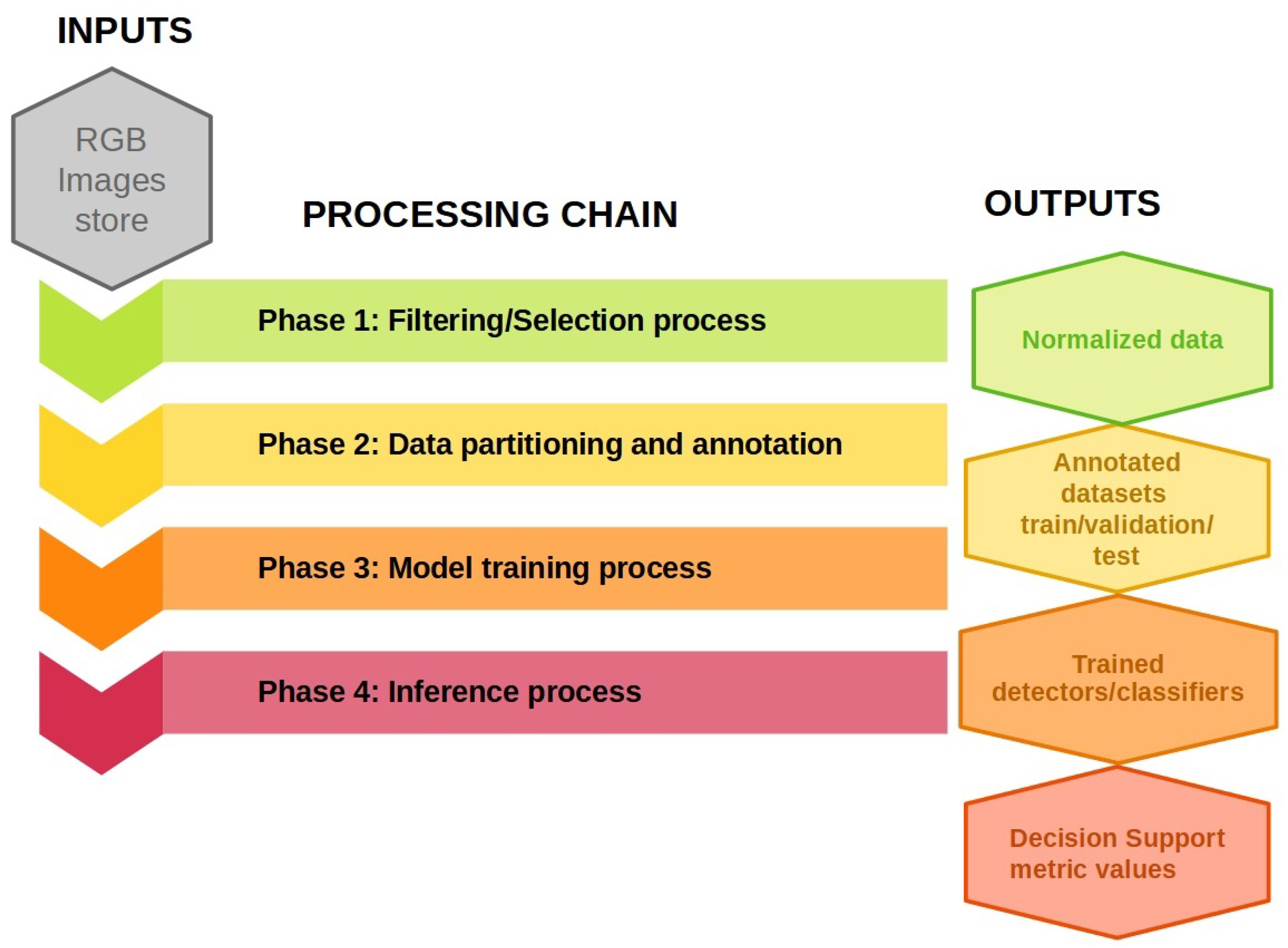
2.1. Proposed Object Detection Framework

The authors propose a framework that uses vine-field RGB cameras as data inputs and tries to detect downy mildew or other vine diseases or viticulture stress caused by extreme environmental conditions at the vine level, similar to their thingsAI implementation [47], by utilizing RGB image data and deep learning object detection models. Their proposition was initially presented at [13] and modified accordingly to support periodic image and real-time video stream inferences. Figure 1 illustrates the authors’ proposed object detection framework.

The proposed detection framework takes RGB data images of vines as input. It comprises four processing phases, each requiring the previous one to have been completed prior to execution. The outputs of each processing phase are inputs for the next, and so forth. This constitutes a chain of independent processing steps that may stop at one level without further processing, providing specific data or metadata outputs. The first phase is the data filtering/data selection process. Normalized image datasets based on specific criteria, features, rules, or time frames are the output of this step. Usually, metadata information is added to the normalized datasets. The second phase includes data partitioning based on unsupervised autoencoders or supervised data annotation or classification tasks. The outputs of phase 2 are the normalized data with the corresponding metadata localization information.

Phase 3 is the model training process. It constructs and produces trained models of complex deep-layer structures, with parameters and biases calibrated via forward and backward operations. The outputs of the training process are models with the best precision—recall scores achieved over a set of iterations of hyperparameter calibration. Finally, phase 4 includes the inference process that loads model structures and parameter values and performs object detections on RGB images or video streams. Object detection outcomes and confidence scores are data inputs for decision support metrics or thresholds that trigger notifications for interventions and alerts for farmers.

The authors’ proposed detection framework functionality has been system-level implemented and is presented by the authors in Section 2.2.

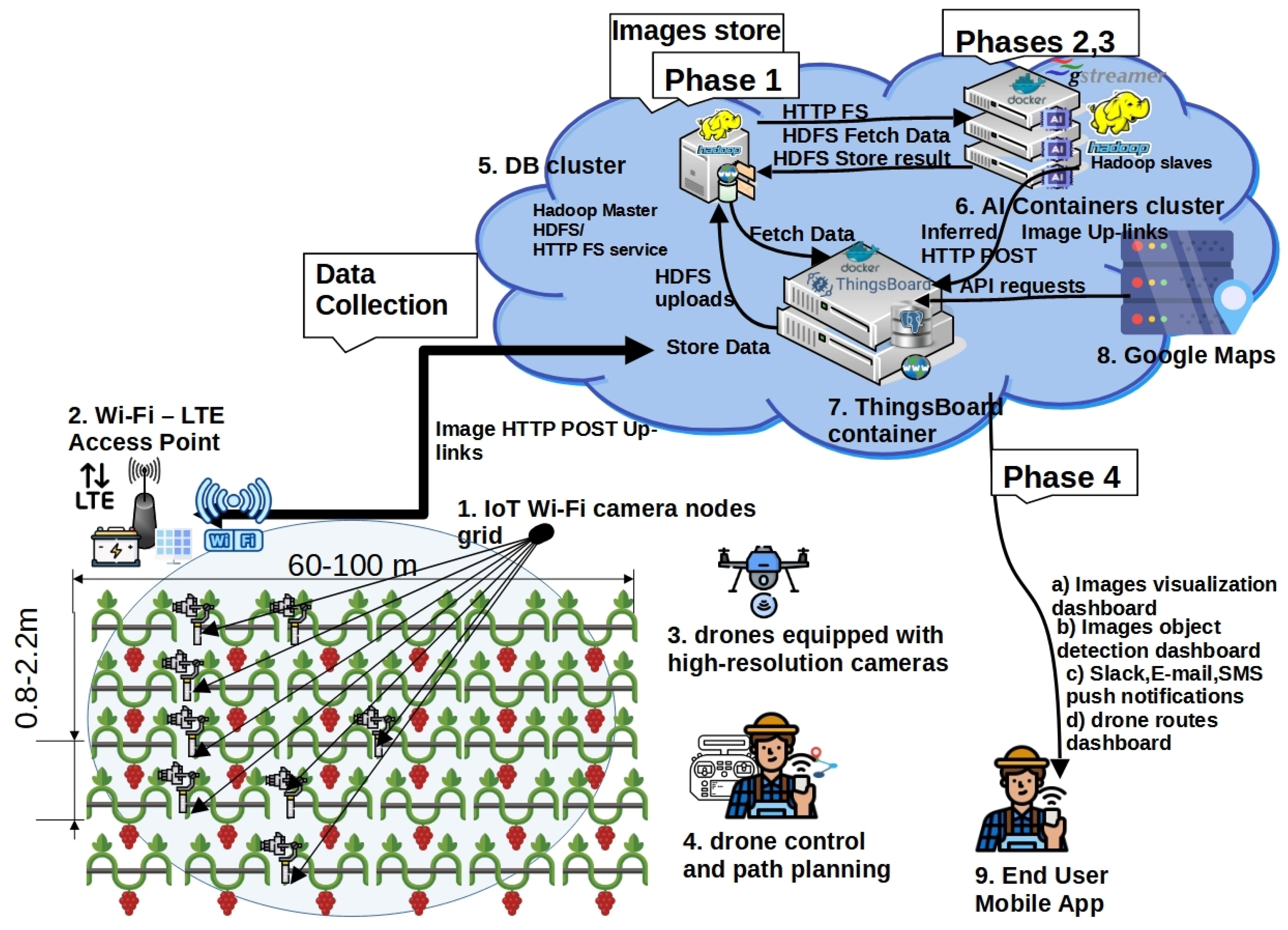
2.2. Proposed High-Level System Architecture Incorporating the Framework

The proposed system architecture that supports the authors’ framework is presented in Figure 2 and includes two arbitrary sources of data acquisition: (1) from the IoT Wi-Fi camera-equipped devices that periodically upload images to the cloud, and (2) from drones with high-resolution cameras that can be set to automatic or semiautomatic path-planned routes and real-time upload image bursts or that can even store short-interval video streams and upload based on an upload-timeout set parameter.

The IoT node devices are illustrated in Figure 3a. Each device includes an AI-thinker ESP32 dual-core module of a 240 MHz Espressif, Shanghai, China, Tensilica LX6 32bit ARM core (see Figure 3a (1)), with 512 KB of RAM and 4 MB of PSRAM. An OmniVision OV2640 2MPixel camera is connected to each IoT device. The OV2640 module can capture images of a maximum size of 1600 × 1200 px. The IoT device also has embedded 2.4 GHz Wi-Fi and Bluetooth 4.2 modules. The IoT device is powered via a 4.2 V 18650 battery pack (see Figure 3a (3)) via a 12 to 3.3 V step-down converter (see Figure 3a (2)), and its battery is directly powered by a 6 V solar panel (see Figure 3a (4)). Each IoT node device operates autonomously using a 3200 mAh 18650 battery and a 2 W/6 V attached panel.

The Wi-Fi-LTE access point (see Figure 2 (2)) includes a Teltonika RUT-240 Wi-Fi access point to LTE gateway device directly powered by a 12 V/100 Ah battery. An 80 W/12 V photovoltaic panel continuously charges the battery via a PWM 12 V charge controller. On the Wi-Fi antenna of the access point device, an additional module of a 2 W/12 V powered signal amplifier is used to boost the 2.4 GHz Wi-Fi signal up to a 2 km coverage range.

The access point board is also connected to a 3G/4G dongle for data uploads to the system’s cloud application services (see Figure 2 (7)). The access point device can cover areas of at least 1–2 km using unidirectional 4–7 dBi antennas and appropriate power-boosting low-noise broadband amplifier circuitry. This increases the coverage radius using a single connection point for signals at 2400–2500 MHz of 7–15 dBm input signal range, thus minimizing maintenance and communication provider costs.

The IoT devices connect to a nearby Wi-Fi access point for cloud imagery data uplinks. The IoT devices are periodically activated using a fixed deep-sleep period of 1–6 h. Upon waking, each IoT uploads captured images by performing HTTP POST uplinks, as illustrated in Figure 2. Moreover, the IoT camera device operates as follows: Once the IoT devices have access point connectivity, they request network time information from the internet Network Time Protocol (NTP) service providers to update their internal system clock. Then, if day hours are detected, the camera module initializes, and the image is captured and stored in the device’s PSRAM. Then, the data are JPEG-compressed and uploaded to the ThingsBoard AS [45] data collector service, using HTTP multipart POSTS of base64 content. Every IoT device has a unique device ID token (UID) for data collector service authentication and image upload. Upon upload completion, the files are stored in the Hadoop file storage cluster, and the appropriate dashboard panel encodes the uploaded base64 file streams to a ThingsBoard dashboard HTML image illustration, as shown in Figure 3b, for visualization purposes.

Similar to ground monitoring IoT camera devices, aerial surveying drones can operate using two different modes: (A) capturing and uploading still images with geolocation information included, acquired by the drone’s GPS receiver, and (B) capturing h.264 video streams transcoded to MOV files with embedded GPS metadata. Both still images and video streams can be directly uploaded to the data collector service using HTTP multipart POST requests. The video streams are of fixed size lengths up to 100 MB to avoid HTTP timeouts. Each video stream HTTP POST uplink is accompanied by drone timestamps and UID information as JSON metadata of the HTTP multipart request. The data collector service can use that as incoming HTTP POST requests’ identification information.

Drone flights must maintain close distances to the vines at the z axis, no more than 3–4 m above them, to have high-resolution leaf imagery data similar to the ones received by the IoT camera nodes. Nevertheless, since altitude offsets provided by APIs are of 20–30 m accuracy in the area of Eastern Europe [11], drones cannot automatically maintain the required minimum z-axis height without human intervention and manual flight corrections. In order to provide automated drone processes at low-altitude passes, the proposed framework sets the following requirements that need to be fulfilled in the surveyed area [48]:

• Aerial LiDaR mapping needs to be performed in the surveyed field area using UAVs as a preprocessing step to create a 3D survey representation. LiDaR instruments can measure the Earth’s surface at sampling pulse rates greater than 200 KHz, offering a point cloud of highly accurate georeferenced elevation points.
• UAVs’ aerial RTK GPS receivers that receive the RTCM correction stream must be utilized. Then, point locations with 1–3 cm accuracy in real time (nominal) must be provided to georeferenced maps or APIs.
• The fundamental vertical accuracy (FVA) of the open data areas measured must be at a high confidence level above 92%.
• The absolute point altitude accuracies of the acquired LiDaR system elevation points must be in the range of 10–20 cm to offer drone flights close to the vines.
• UAV mappings of vegetation areas need to be performed with the concurrent utilization of multispectral cameras in the near-infrared band of 750–830 nm so as to detect and exclude non viticulture areas of low or high refractivity by performing post processing NDVI metric calculations [49] on map layers.
• Using EU-DEM [11] as a base altitude reference, appropriate altitude corrections must be made to the GIS path-planning map grid. Then, the surveying drones need to perform periodic HTTP requests to acquire sampling altitude corrections. If viticulture fields’ surface altitude variances are no more than 0.5–1 m in grid surface areas of at least 1–5 km, then with the exception of dense plantation areas (such as forests, provided by NDVI measurements), the altitude values can be set as a fixed vertical parameter value of drone altitude offset for the specific survey areas.

Following the above guidelines, we may offer automated drone low-altitude image acquisition based on predefined path plans on map layers.

The data collector service implements phase 1 of our proposed framework. It is a standalone HTTP service based on the HTTP Python3 uploadserver module. This service is instantiated on a custom docker container created by the authors [46], where the ThingsBoard AS also resides. The data collector accepts still images or video stream uploads. Then, based on the device UID and date–time information, it forwards the image data to both the ThingsBoard AS for visualization purposes (see Figure 3b) and the distributed Hadoop file storage cluster via its master node [43,44].

The phase 2 framework data annotation process is performed using AI containers (see Figure 2 (6)). AI containers responsible for data annotation are the AI client containers, that is, custom dockerized Linux boxes [46] with remote X-server access and direct access to the HDFS file system (see Figure 2 (5)). The annotation process is supervised remotely by experts using appropriate annotation tools [50]. After image annotation, the images are appropriately resized for model training processes. Annotated box coordinates stored in XML files are automatically extracted and corrected for any image size given or selected during training. Upon image object-class annotation, the client AI containers execute phase 3 model training tasks. The final trained models are also stored in the HDFS file system.

Inference AI clusters perform phase 4 framework inferences. Such clusters instantiate agents that download the previously trained object detection models using the method GET on the HTTP-HDFS service [51] of the DB cluster so as to perform object inference processes on either uploaded images or video streams. Then, upon detection inference completion, they upload the new images with the inference boxes to the ThingsBoard AS [45] by performing HTTP POST requests or delivering the real-time inference-annotated video stream via RTSP/RTP streams (see Figure 4c) with the use of the GStreamer API [52].

Finally, the ThingsBoard platform [45] can be used for detection visualization (see Figure 3c,d); for GPS drone path-plan visualization (see Figure 4b) taken from the images’ EXIF metadata information [53]; and to issue alerts or notifications based on AI container inferences and inferred metadata over Slack, SMS, email, or other external push notification services. The following Section 3 presents the authors’ experimentation of their implemented system for detecting downy mildew and evaluating different YOLO and Faster R-CNN models.

3. Experimental Scenario

The authors experimented in their debina variety viticulture field in Zitsa, Epirus, Greece, as illustrated in Figure 4b. The experimental setup included the installation of ten vine-field IoT camera devices, as illustrated in Figure 3a, in the middle of every second row in the viticulture field at a distance of 40–60 cm from the vine leaves.

The IoT camera nodes forwarded field images to the ThingsBoard cloud platform container. Each IoT device’s 2MPixel camera could capture hourly 1024 × 768 px, 810 KB frame buffer images during daytime, compressed to 190–230 KB JPEG images and uploaded to the ThingsBoard platform using base64 HTTP POSTS. The experiment was performed from May to August 2023.

Furthermore, weekly images were captured from June–July 2023 using a DJI Mavic 3 Pro drone equipped with a GPS receiver and a 20MPixel camera, as illustrated in Figure 4a, capable of capturing 3264 × 2448 px images of 7 MB JPEG compressed image size every 2 s, as well video records. GPS information was included in each image as EXIF location metadata during drone vine passes [53]. Figure 4b illustrates the geolocation metadata latitude and longitude EXIF image values of a drone pass acquiring 240 images, using the Python3-exif package and the ThingsBoard platform’s Google Maps module. Figure 4c illustrates the drone image inference result using the YOLOv5 model, while Figure 5(1,2) illustrate the image inference results of ResNet-50 and ResNet-152 model implementations, accordingly [54].

For the year 2023, a downy mildew outburst occurred due to increased levels of rainfall, specifically in May and June. The authors performed no downy mildew interventions, closely monitored the disease’s secondary infection cycles’ progress, and collected photos from the ground-based cameras and drones. The first infections became apparent with a small number of sporangia incubating at the backs of some leaves on 1st of June. What followed was a catastrophic collapse. At least one oil spot/tree appeared by 12 June, the first signs of the disease on the fruit appeared by 20 June, and by 30 June, the whole fruit had reached necrosis, with most of the leaves/vines having oil spots all over. The resulting productivity collapse for the year 2023 characterizes these conditions as a significant mildew outburst case. In addition, 2023 has been described as a year of mildew outbursts in Zitsa, in which most nearby farmers did not manage to maintain their vine yield. A few that did were forced to perform seven to eight interventions from May until the end of August to save 70–80% of their production, while farmers that performed five to seven interventions managed to save 30–50% of their vine production, accordingly.

The authors collected a dataset containing a total number of 6800 photos from drones and ground-field cameras. Then, part of the dataset was leaf-annotated using the labeling tool [50], and the images were resized accordingly based on the sizes mentioned in

Table 1. Trained models’ input sizes, number of trainable parameters, and estimated model sizes. The table is horizontally line-split into two parts. The first part includes models with many trainable parameters (size > 100 M) used for cloud inferences. The second part includes models used by embedded devices or mobile phone applications.

Trained Model	JPEG Compressed Image Input Sizes (W × H, MB)	No Trainable Parameters	Estimated Model Sizes (MB)
ResNet-152	(640 × 640, 0.49)	199,874,714	980
ResNet-101	(640 × 640, 0.49)	184,231,066	704
YOLOv3-Darknet	(640 × 640, 0.49)	84,364,442	338.5
EfficientNet-b0	(640 × 640, 0.49)	84,141,782	337
FRCNN-VGG16	(640 × 640, 0.49)	43,877,530	168
ResNet-50	(640 × 640, 0.49)	41,304,286	159
YOLOv5-small (YOLOv5s)	(640 × 640, 0.49)	7,468,160	101.5
SqueezeNet	(4128 × 4128, 3.6)	29,876,890	98
ViTDet-tiny	(4128 × 4128, 3.6)	22,786,382	87
MobileNetV3	(4128 × 4128, 3.6)	18,935,354	73
YOLOv8-nano (YOLOv8n)	(4128 × 4128, 3.6)	3,151,904	29.8

for each experimentation model class. For this experimental scenario, 1200 images were annotated with at least 7–10 annotations/image using two classes: normal class leaves and leaves or leaf parts containing mildew oil spots or deformations. A total number of around 9800 labeled bounding boxes were labeled. The annotations were saved in PASCAL VOC XML used by Faster R-CNN models and YOLO JSON formats using the Roboflow annotations transformation tools [55]. PyTorch torchvision was used to train the Faster R-CNN models [56], and the Ultralytics platform and Python API were used to train the YOLO models [57].

The experimentally trained models were divided into two model classes that were separately examined: (1) the cloud-based object detectors class, and (2) the device-embedded detectors class. The distinctive point among the two classes was the model size that needs to be memory-resident for each detection. Cloud-based detector model sizes are above 100 MB and can provide as a service from 1 second/frame up to 30 seconds/frame of concurrent image detection inferences using cloud host virtual machines of at least 16-core ARM-based Ampere A1 cores and 16 GB of RAM [58]. On the other hand, embedded detectors are device-level instantiated inferences in mobile phones or embedded IoT devices that are usually small-sized models of less than 100 MB so that the model can load in the device-restricted memory resources (from 256 MB up to 4 GB of allowed maximum process memory and four to eight ARM cores available). Table 1 shows each trained model used and the weight parameters’ storage sizes for these two distinct classes.

Evaluation Metrics

This experimentation uses the mean average precision and loss evaluation metrics for model evaluation. Object detection inferences output bounding boxes of detected contours of objects with their corresponding confidence class level values. The models perform two main tasks on the generated image feature maps. The classification task that checks whether a detected object exists in the image, using the maximum class probability to denote the detected confidence level provided by the location of the detected object’s bounding box concerning the ground-truth annotation, is calculated by the intersection over union (IoU) metric as a locality parameter. The IoU metric is calculated based on Equation (1).

$$IOU=\frac{area(A_p\cap A_{GT})}{area(A_p\cup A_{GT})}$$

(1)

where $A_p$ is the detected bounding box area and $A_{GT}$ is the annotated leaves ground-truth area (area of overlap over the detected boxes). Using the IoU threshold value of 0.5 to denote true-positive inferences, the mean average precision (mAP) value is calculated per test image using all points’ (object detection indices $i=1\dots n$ of m classes) interpolation calculation as derived from Equation (2) [59].

$$mA{P}_{\alpha =0.5}=\frac{1}{m}\sum _{c=1}^m\sum _i^n(r_{i+1}-r_i)P_{intp}\left(r_{i+1}\right)=\frac{1}{m}\sum _{c=1}^m\sum _i^n(r_{i+1}-r_i)\underset{r^{\prime }:r^{\prime }\ge r_{i+1}}{max}P\left(r^{\prime }\right)$$

(2)

where $\alpha =0.5$ is the level threshold, $P_{intp}$ is the interpolated precision value for a detection calculated as $P=\frac{TP}{TP+FP}=\frac{TP}{alldetections}$, r is the recall value for a detection calculated as $r=\frac{TP}{TP+FN}=\frac{TP}{allgroundtruths}$, $P\left(r^{\prime }\right)$ is precision measured at recall $r^{\prime }$, m is the number of the object detection classes, and $i=1\dots n$ is the index of the detected boxes. Three types of losses are commonly considered: train box, classification, and object loss. Train box loss is the mean squared error bounding box regression loss; the confidence of objects’ presence is the object loss; and classification loss is the cross-entropy loss.

The train box loss represents how well the algorithm can locate an actual object by measuring how much the predicted bounding box is misplaced over a ground-truth object by calculating the mean sum of the n detected true-positive and false-positive IoU values based on Equation (3).

$$Los{s}_{TB}=\frac{1}{T{P}_b+F{P}_b}\sum _i^n(1-Io{U}_i+\frac{p^{2}d|b^p,b^{gt}|}{{\lambda }^2})$$

(3)

where $d|b^p,b^{gt}|$ is the distance of the central points of predicted and actual boxes, p is the predicted maximum value, and $\lambda$ represents the diagonal length of the smallest enclosing box covering the two boxes [60].

The object loss is expressed by Equation (4). It is defined as the ratio of the absolute difference between the number of annotated image objects N minus the true-positive detections m expressed by confidence scores over the annotated objects, where the confidence score $C{s}_i$ of the i detected object is expressed by the probability that the i anchor box contains an object.

$$Los{s}_{OBJ}=\frac{{\displaystyle |N-\sum _{i=1}^{m}C{s}_i|}}{N}$$

(4)

Classification loss is the cross-entropy on the object prediction probability vector calculated using Equation (5)

$$Los{s}_{CLS}=-\sum _{x}p\left(x\right)·ln\left(q(x;\theta )\right)=-ln\left(q(C_i;\theta )\right)$$

(5)

where p is the ground-truth classification probability vector of an image object detection x, q is the detected probability vector values of x, $q\left(C_i\right)$ is the detection vector probability value of the ground-truth maximum likelihood class $C_i$, and $i=1\dots n$ is the number of distinct classes. The use of either $lo{g}_2$ or $ln$ in Equation (5) is arbitrary depending on the loss measurement unit (bits or nats). Parameter $\theta$ expresses the hyperparameter values used by the model.

Table 1 shows the examined models, trainable parameters, and sizes. Figure 6 illustrates the labelImg tool [50] annotation tasks, using images acquired by either (a) the IoT devices or (b) drones. The dataset images were obtained in May–July 2023 during a downy mildew outburst in Zitsa, Greece. The annotated dataset was split 20–80% as validation and training sets. An additional 300 images (1200 + 300) were kept separate for the models’ testing. Part of the IoT nodes annotated dataset is available online at [61]. The selected images for either training or inference from the IoT nodes and drones were collected during midday hours of minimum cloudiness (cloud coverage up to 40%) and wind speeds of less than 5 km/h. After image annotation, these IoT node images were used along with the captured drone images, which were resized to 4128 × 4128 px or 640 × 640 px during model training. During training, the annotated box coordinates stored in XML files were automatically extracted and corrected for any image size given or selected.

The models’ evaluation was performed using the following methodology. First, a model class distinction was performed based on the stored model size in MB. The large models with sizes above 100 MB were placed in the cloud-based models class. Cloud-based models usually reside in cloud services, offering inferences as a service. These models have many trainable parameters and a small image input size to decrease inference processing time latencies, thus improving interactivity. On the other hand, the embedded models class of less than 100 MB model sizes can load on mobile devices for edge computing inferences. Such models have been trained to use the maximum image sizes captured by drone and IoT cameras. In these models, we tried to retain as much information as possible since the embedded devices can afford some extra processing efforts due to their small model sizes. When input images share a comparable set of features, their matching accuracy is substantially increased, while the reduction in image size facilitates faster processing but may compromise accuracy. So, the images of bigger sizes are set as a trade-off for the small number of model parameters that affect model accuracy results. Cloud and embedded models are evaluated separately; the results are presented in Section 4.

According to Table 1, ResNet-152 and YOLOv5-small (YOLOv5s) were the biggest and smallest cloud models, accordingly. SqueezeNet v1.1 [62] was the biggest for mobile and embedded devices, occupying 98 MB of memory during inferences, while YOLOv8 nano required only 30 MB. The following Section 4 presents the models’ evaluation results.

4. Experimental Results and Discussion

The experimental results are also presented based on the previously mentioned class distinction of cloud and embedded-device models. First, the $mA{P}_{0.5}$ values are examined, then $mA{P}_{0.5:0.95}$, and, finally, model losses following a hierarchical evaluation methodology. At first, we use the maximum number of epochs for each model; if the $mA{P}_{0.5}$ values’ difference between two tested models is less than 5%, then further evaluation is performed using $mA{P}_{0.5:0.95}$, which is the mean of mAP values using IoU threshold values of 0.5 up to 0.95 with a threshold step of 0.05. The model’s loss curves are also considered to examine each model’s classifier capabilities. Since models may use different box loss functions, only classification losses are used for cross-comparison results if box losses are close to zero or significantly smaller than classification losses. If a model has minimum classification losses and presents a low mAP value, then object losses are the reason for its poor performance.

Table 2. $mA{P}_{0.5}$ values over 20, 50, and 100 training epochs for both embedded and cloud Faster R-CNN and YOLO models.

Model	${\mathit{mAP}}_{0.5}$-20 Epochs	${\mathit{mAP}}_{0.5}$-50 Epochs	${\mathit{mAP}}_{0.5}$-100 Epochs
ResNet-152	0.9934	0.995	0.9951
ResNet-101	0.989	0.995	0.995
ResNet-50	0.65	0.92	0.9949
EfficientNet-b0	0.29	0.68	0.868
FRCNN-VGG16	0.9944	0.9949	0.995
YOLOv3-Darknet	0.26	0.78	0.94
YOLOv5-small (YOLOv5s)	0.92	0.92	0.96
SqueezeNet	0.558	0.783	0.981
ViTDet-tiny	0.16	0.55	0.901
MobileNetV3	0.37	0.64	0.99
YOLOv8-nano (YOLOv8n)	0.86	0.91	0.94

presents the $mA{P}_{0.5}$ values for each examined model.

Examining the cloud models, from Table 2, the ResNet models’ $mA{P}_{0.5}$ output results for 100 training epochs are similar, so further evaluation using $mA{P}_{0.5:0.95}$ values and classification losses are further examined below. FRCNN-VGG16 also presents $mA{P}_{0.5}$ values close to the ResNet models for 100 epochs that require further examination. The same applies to the YOLO models. The EfficientNet-b0 model [63] did not present $mA{P}_{0.5}$ values close to all other cloud models, having 8% fewer values than the least $mA{P}_{0.5}$ value achieved by the YOLOv3 model. The authors mark such values as significantly low in terms of performance, and therefore, the EfficientNet-b0 model is not further examined. Figure 7 shows the $mA{P}_{0.5:0.95}$ values achieved by the cloud models over training epochs.

From the examined cloud models, ResNet models presented the best $mA{P}_{0\_5:0\_95}$ results, followed by the VGG16 Faster R-CNN model. All examined Faster R-CNN models outperformed the YOLOv5 model, achieving at least 10% better accuracy. YOLOv3 scored the minimum precision value for 100 epochs, and it was outperformed up to 22% by YOLOv5 for 100 training epochs. In addition, YOLOv5 was outperformed by the less accurate ResNet model, ResNet-50, by 13% and by the Faster R-CNN-VGG16 model by 10% for 100 training epochs. Nevertheless, YOLOv5 is considered a fast cloud alternative for video stream inferences (see

Table 3. Inference time values, expressed in frames per second (FPS), for inference of h.264 drone video streams, resized to 640 × 640 px and 4128 × 4128 px sizes of image frames for cloud and embedded Faster R-CNN and YOLO models, accordingly.

Model	Achieved Mean FPS	${\mathit{mAP}}_{0.5:0.95}^{\mathit{Epochs}=100}$
ResNet-152	0.262	0.9476
ResNet-101	0.321	0.9411
ResNet-50	0.511	0.940
FRCNN-VGG16	0.404	0.9106
YOLOv3-Darknet	0.591	0.633
YOLOv5-small (YOLOv5s)	1.28	0.812
SqueezeNet	1.645	0.789
ViTDet-tiny	0.517	0.622
MobileNetV3	3.24	0.876
YOLOv8-nano (YOLOv8n)	2.08	0.84

), as it is at least 60% faster than any Faster-R-CNN model expressed by mean processed frames per second (FPS). Comparing ResNet models of 50, 101, and 152 residual blocks in terms of $mA{P}_{0.5:0.95}$ values for 100 training epochs, a minimum accuracy increase of 3% was presented between ResNet-101 and ResNet-50, and no significant accuracy increases were spotted above 1% between ResNet-152 and ResNet-101. That is, the smallest but faster ResNet-101 can provide almost the same inference results with a ResNet-152 model 18–20% faster (see Table 3). Figure 8 presents the classification loss for cloud models expressed using Equation (5).

As shown in Figure 8, classification losses drop around 30% between ResNet-50 and the ResNet-101 and ResNet-152 models for 100 epochs. Additionally, classification losses for ResNet-50 are 17.9–20% higher than the Faster R-CNN VGG16 model. Finally, the YOLOv3 model presents significantly low classification losses for training epochs above 70, close to the ResNet-50 values and lower than the YOLOv5 classification losses. This indicates the significant localization losses of the YOLOv3 model as the number of epochs increases due to its low classification loss output results with respect to the low achieved $mA{P}_{0.5:0.95}$ values.

Examining the embedded models, from Table 2, all models present $mA{P}_{0.5}$ values for 100 training epochs of value differences of no more than 5%. So, all models are further evaluated. Figure 9 presents the $mA{P}_{0.5:0.95}$ values achieved by the embedded models over training epochs.

From Figure 9, the MobileNetV3 model [64] presented the best $mA{P}_{0.5:0.95}$ precision value of 87%, 2.7–3% better than YOLOv8n of 84.4% precision value. The maximum number of epochs used in the training of YOLOv8n was 100, indicated as the default parameter by [57]. Nevertheless, due to the linear decrease of the classification loss curve of YOLOv8n, as shown in Figure 10, more training epochs may be required to achieve significant results (100–600 epochs), as mentioned by [65]. YOLOv8 also underachieves in terms of speed, around 35% less than MobileNetV3, thus making MobileNetV3 the most accurate and fast embedded object detection model, followed by YOLOv8n and then the SqueezeNet model. Embedded models yield smaller accuracies than cloud models, achieving up to 87.6% $mA{P}_{0.5:0.95}$ maximum precision value for 100 training epochs of the MobileNetV3 model in comparison to the Faster R-CNN ResNet-152 model of 0.947% precision value. Moreover, YOLOv5s outperforms the YOLOv8n model in terms of precision for 100 training epochs by 8%.

Figure 10 illustrates classification losses of the embedded models. Figure 10 shows that ViTDet-tiny [66] fails to adequately perform, presenting $mA{P}_{0.5:0.95}$ precision values below 60% due to significant classification losses. MobileNetV3 presents the least losses, which decrease nonlinearly over epochs, while the SqueezeNet model maintains a linearly decreasing classification loss curve over epochs, with more losses than the MobileNetV3 model. The YOLOv8n model, until 50 epochs, significantly decreases its classification loss more than MobileNetV3. However, above 50 epochs, its classification loss starts to fluctuate above MobileNetV3 losses and close to the SqueezeNet model values. This fluctuation of the classification loss values of YOLOv8n above 50 epochs is the main reason for its under accuracy performance concerning the MobileNetV3 model.

Taking our experimentation one step further, a drone-acquired h.264 video stream of 3.450 GB size and 3840 × 2160 px frames resolution, transformed during inference to 640 × 640 px and 4128 × 4128 px sized frames, accordingly, was used to compare forward-pass times among models. Each of the examined models was used to provide bounded object detection of a confidence level value of 0.2 for each one of the video stream frames, and the average frames per second (FPS) values were calculated. Table 3 presents these results. The experimental system used for providing inference times expressed as frames per second (FPS) was an Intel Xeon E5-1620v3, quad-core, with two threads/core, a total of nine logical CPUs, and 32 GB of DDR4 memory size.

It is evident from Table 3 that for the cloud models, YOLOv5s has the highest FPS value, followed by ResNet-50 and then FR-CNN-VGG16, also based on the hierarchical maximum achieved $mA{P}_{0.5:0.95}$ values for 100 training epochs. Examining the speed of ResNet-50, compared to the other deeper ResNet models, ResNet-101 is 37% slower than ResNet-50, while ResNet-152 is 48.7% slower than ResNet-50. As the network blocks double, inference speeds drop around 24%. YOLOv3 models fail to perform well in speed and accuracy compared to YOLOv5. Finally, FR-CNN-VGG16 does not perform better than ResNet-50 in terms of speed and accuracy. From the cloud models tested, only the YOLOv5s model acquired close to real-time inference capabilities above 1 FPS, as highlighted in Table 3.

From the embedded models, MobileNetV3 achieved the best accuracy and speed results. YOLOv8n achieved 35% less speed and 2.7–3% less accuracy than MobileNetV3, followed by SqueezeNet’s speed of 49.3% less than MobileNetV3. Nevertheless, the MobileNetV3, YOLOv8, and SqueezeNet models achieved close to real-time accuracies above 1 FPS in contrast to the ViTDet-tiny model speed results that underperformed, providing inference speed times close to the ones of the ResNet-50 cloud model. For embedded models, YOLOv8 models are 30–65% faster than their YOLOv5 predecessors (in our experimentation 38.5%). Nevertheless, YOLOv8 did not manage to exceed the inference speeds of the MobileNetV3 model. The SqueezeNet model presents two times slower inference speeds than MobileNetV3 and 6% less accuracy results than the YOLOv8n model. The authors conclude that Mobilevenv3 is the best embedded model in terms of accuracy and speed, followed by the YOLOv8 and SqueezeNet models.

5. Conclusions

This paper presents a new framework for detecting downy mildew disease spreads in viticulture, using RGB image inputs from ground IoT camera devices and drones. The authors present their proposed framework phases and their corresponding phase outputs. The authors also present a cloud-based system following their framework implementation. The system’s capabilities include cloud-distributed data collection and object detection of vine fungal diseases via training and object detection services. The authors also implemented an automated IoT camera node for vine-field imagery data acquisition and an automated process of object-detecting video streams acquired from RGB camera-equipped drones. Furthermore, they also set the necessary guidelines to achieve automated drone aerial path routing and real-time inferencing.

The proposed system of low-cost and autonomous IoT devices can periodically collect images and detect downy mildew spreads at the plant level. The system’s application services can use deep learning model object detection to notify farmers of the extent of the disease at the vine level, providing targeted field interventions or pesticide use. Similarly, if IoT device deployment is not feasible, periodic drone flights can be used to acquire imagery data inputs of GPS metadata and offer the same detection and alerting capabilities.

The authors experimented with their system, using it for the process of training object detection models using a downy mildew outburst experimental dataset acquired in 2023 at the viticulture area of protected designation of origin Debian grape variety in Zitsa, Greece, on two distinct detection cases: (a) cloud-enabled low-resolution detection of big-depth models, where the model training and inferences are performed in the cloud, and (b) embedded fast inference models of high-resolution image inputs, which are cloud-trained but executed at the device level.

From the cloud-enabled models’ experimentation and the comparison between Faster R-CNN and YOLOv5 models, Faster R-CNN ResNet and VGG16 models outperformed YOLO. In contrast, YOLOv5 outperformed cloud Faster R-CNN models by 35–75% in terms of speed inferences in video streams. Moreover, deep ResNet-152 outperformed the ResNet-101 and ResNet-50 models. Nevertheless, regarding video stream inferences, the ResNet-152 model underachieved by close to 18% in terms of FPS concerning ResNet-101, provided that the ResNet-152 accuracy results are no more than 0.6% better than the ones achieved by the ResNet-101 model. Finally, the 60–75% better speed of the YOLOv5s with respect to the ResNet-101 model is significant, but as a model, it still needs to be more accurate than the ResNet-101 Faster R-CNN model that achieved at least 13.8% higher precision results. From the embedded model’s experimentation, Faster R-CNN MobileNetV3 outperformed YOLOv8n by 2.7–3% in terms of accuracy, and it was 35% faster in inference speeds.

The proposed system implements a low-maintenance, low-cost architecture of self-sustained IoT nodes that utilizes deep learning models to detect downy mildew events. However, the system’s limitations include the efforts needed to deploy and periodically check the IoT device nodes’ proper functionality and vine image acquisition, as well as the functionality of the Wi-Fi gateway node. Similarly, for drone-surveyed image acquisition, appropriate guidelines mentioned by the authors must be fulfilled to function properly. The authors set the models’ hyperparameter tuning towards downy mildew and the use of their proposed system for detecting other fungal diseases of powdery mildew and gray mold in vine fields as future work.

References

1. Sapaev, J.; Fayziev, J.; Sapaev, I.; Abdullaev, D.; Nazaraliev, D.; Sapaev, B. Viticulture and wine production: Challenges, opportunities and possible implications. E3S Web Conf. 2023, 452, 01037. [Google Scholar] [CrossRef]
2. Peladarinos, N.; Piromalis, D.; Cheimaras, V.; Tserepas, E.; Munteanu, R.A.; Papageorgas, P. Enhancing Smart Agriculture by Implementing Digital Twins: A Comprehensive Review. Sensors 2023, 23, 7128. [Google Scholar] [CrossRef] [PubMed]
3. Bove, F.; Savary, S.; Willocquet, L.; Rossi, V. Designing a modelling structure for the grapevine downy mildew pathosystem. Eur. J. Plant Pathol. 2020, 157, 251–268. [Google Scholar] [CrossRef]
4. Velasquez-Camacho, L.; Otero, M.; Basile, B.; Pijuan, J.; Corrado, G. Current Trends and Perspectives on Predictive Models for Mildew Diseases in Vineyards. Microorganisms 2022, 11, 73. [Google Scholar] [CrossRef]
5. Rossi, V.; Caffi, T.; Gobbin, D. Contribution of molecular studies to botanical epidemiology and disease modelling: Grapevine downy mildew as a case-study. Eur. J. Plant Pathol. 2013, 135, 641–654. [Google Scholar] [CrossRef]
6. Caffi, T.; Gilardi, G.; Monchiero, M.; Rossi, V. Production and release of asexual sporangia in Plasmopara viticola. Phytopathology 2013, 103, 64–73. [Google Scholar] [CrossRef]
7. Vanegas, F.; Bratanov, D.; Powell, K.; Weiss, J.; Gonzalez, F. A Novel Methodology for Improving Plant Pest Surveillance in Vineyards and Crops Using UAV-Based Hyperspectral and Spatial Data. Sensors 2018, 18, 260. [Google Scholar] [CrossRef]
8. Li, Y.; Shen, F.; Hu, L.; Lang, Z.; Liu, Q.; Cai, F.; Fu, L. A Stare-Down Video-Rate High-Throughput Hyperspectral Imaging System and Its Applications in Biological Sample Sensing. IEEE Sens. J. 2023, 23, 23629–23637. [Google Scholar] [CrossRef]
9. Lacotte, V.; Peignier, S.; Raynal, M.; Demeaux, I.; Delmotte, F.; Da Silva, P. Spatial–Spectral Analysis of Hyperspectral Images Reveals Early Detection of Downy Mildew on Grapevine Leaves. Int. J. Mol. Sci. 2022, 23, 10012. [Google Scholar] [CrossRef]
10. Pithan, P.A.; Ducati, J.R.; Garrido, L.R.; Arruda, D.C.; Thum, A.B.; Hoff, R. Spectral characterization of fungal diseases downy mildew, powdery mildew, black-foot and Petri disease on Vitis vinifera leaves. Int. J. Remote Sens. 2021, 42, 5680–5697. [Google Scholar] [CrossRef]
11. EU-DEM. EU-DEM-GISCO-Eurostat. 2023. Available online: https://ec.europa.eu/eurostat/web/gisco/geodata/reference-data/elevation/eu-dem (accessed on 10 December 2023).
12. Abdelghafour, F.; Keresztes, B.; Germain, C.; Da Costa, J.P. In Field Detection of Downy Mildew Symptoms with Proximal Colour Imaging. Sensors 2020, 20, 4380. [Google Scholar] [CrossRef]
13. Kontogiannis, S.; Asiminidis, C. A Proposed Low-Cost Viticulture Stress Framework for Table Grape Varieties. IoT 2020, 1, 337–359. [Google Scholar] [CrossRef]
14. Zhang, Z.; Qiao, Y.; Guo, Y.; He, D. Deep Learning Based Automatic Grape Downy Mildew Detection. Front. Plant Sci. 2022, 13, 872107. [Google Scholar] [CrossRef] [PubMed]
15. Girshick, R.; Donahue, J.; Darrell, T.; Malik, J. Rich feature hierarchies for accurate object detection and semantic segmentation. arXiv 2014. [Google Scholar] [CrossRef]
16. Sermanet, P.; Eigen, D.; Zhang, X.; Mathieu, M.; Fergus, R.; LeCun, Y. OverFeat: Integrated Recognition, Localization and Detection using Convolutional Networks. arXiv 2014. [Google Scholar] [CrossRef]
17. Ren, S.; He, K.; Girshick, R.; Sun, J. Faster R-CNN: Towards Real-Time Object Detection with Region Proposal Networks. arXiv 2016. [Google Scholar] [CrossRef] [PubMed]
18. Girshick, R. Fast R-CNN. arXiv 2015. [Google Scholar] [CrossRef]
19. Krizhevsky, A.; Sutskever, I.; Hinton, G.E. ImageNet Classification with Deep Convolutional Neural Networks. In Advances in Neural Information Processing Systems; Curran Associates, Inc.: New York, NY, USA, 2012; Volume 25, pp. 1097–1107. ISBN 978-1-62748-003-1. [Google Scholar]
20. Muhammad, U.; Wang, W.; Chattha, S.P.; Ali, S. Pre-trained VGGNet Architecture for Remote-Sensing Image Scene Classification. In Proceedings of the 2018 24th International Conference on Pattern Recognition (ICPR), Beijing, China, 20–24 August 2018; Volume 1, pp. 1622–1627. [Google Scholar] [CrossRef]
21. Bagaskara, A.; Suryanegara, M. Evaluation of VGG-16 and VGG-19 Deep Learning Architecture for Classifying Dementia People. In Proceedings of the 2021 4th International Conference of Computer and Informatics Engineering (IC2IE), Depok, Indonesia, 14 September 2021; Volume 1, pp. 1–4. [Google Scholar] [CrossRef]
22. He, K.; Zhang, X.; Ren, S.; Sun, J. Deep Residual Learning for Image Recognition. arXiv 2015. [Google Scholar] [CrossRef]
23. Szegedy, C.; Vanhoucke, V.; Ioffe, S.; Shlens, J.; Wojna, Z. Rethinking the Inception Architecture for Computer Vision. arXiv 2015. [Google Scholar] [CrossRef]
24. Szegedy, C.; Ioffe, S.; Vanhoucke, V.; Alemi, A. Inception-v4, Inception-ResNet and the Impact of Residual Connections on Learning. arXiv 2016. [Google Scholar] [CrossRef]
25. Anwar, A. Difference between alexnet, vggnet, resnet and inception. Medium-Towards Data Sci. 2019. Available online: https://towardsdatascience.com/the-w3h-of-alexnet-vggnet-resnet-and-inception-7baaaecccc96 (accessed on 15 March 2021).
26. Iandola, F.N.; Han, S.; Moskewicz, M.W.; Ashraf, K.; Dally, W.J.; Keutzer, K. SqueezeNet: AlexNet-level accuracy with 50× fewer parameters and <0.5 MB model size. arXiv 2016. [Google Scholar] [CrossRef]
27. Tan, M.; Le, Q.V. EfficientNet: Rethinking Model Scaling for Convolutional Neural Networks. arXiv 2020. [Google Scholar] [CrossRef]
28. Sandler, M.; Howard, A.; Zhu, M.; Zhmoginov, A.; Chen, L.C. MobileNetV2: Inverted Residuals and Linear Bottlenecks. arXiv 2019. [Google Scholar] [CrossRef]
29. Howard, A.; Sandler, M.; Chu, G.; Chen, L.C.; Chen, B.; Tan, M.; Wang, W.; Zhu, Y.; Pang, R.; Vasudevan, V.; et al. Searching for MobileNetV3. arXiv 2019. [Google Scholar] [CrossRef]
30. Li, Y.; Mao, H.; Girshick, R.; He, K. Exploring Plain Vision Transformer Backbones for Object Detection. arXiv 2022. [Google Scholar] [CrossRef]
31. Redmon, J.; Divvala, S.; Girshick, R.; Farhadi, A. You Only Look Once: Unified, Real-Time Object Detection. arXiv 2016. [Google Scholar] [CrossRef]
32. Liu, W.; Anguelov, D.; Erhan, D.; Szegedy, C.; Reed, S.; Fu, C.Y.; Berg, A.C. SSD: Single Shot MultiBox Detector. In Proceedings of the Computer Vision–ECCV, Amsterdam, The Netherlands, 11–14 October 2016; Leibe, B., Matas, J., Sebe, N., Welling, M., Eds.; Lecture Notes in Computer Science. Springer International Publishing: Berlin/Heidelberg, Germany, 2016. [Google Scholar] [CrossRef]
33. Redmon, J.; Farhadi, A. YOLOv3: An Incremental Improvement. arXiv 2018. [Google Scholar] [CrossRef]
34. Wang, H.; Zhang, F.; Wang, L. Fruit Classification Model Based on Improved Darknet53 Convolutional Neural Network. In Proceedings of the 2020 International Conference on Intelligent Transportation, Big Data and Smart City (ICITBS), Vientiane, Laos, 11–12 January 2020; Volume 1, pp. 881–884. [Google Scholar] [CrossRef]
35. Liu, H.; Sun, F.; Gu, J.; Deng, L. SF-YOLOv5: A Lightweight Small Object Detection Algorithm Based on Improved Feature Fusion Mode. Sensors 2022, 22, 5817. [Google Scholar] [CrossRef]
36. Lyu, C.; Zhang, W.; Huang, H.; Zhou, Y.; Wang, Y.; Liu, Y.; Zhang, S.; Chen, K. RTMDet: An Empirical Study of Designing Real-Time Object Detectors. arXiv 2022. [Google Scholar] [CrossRef]
37. e Hani, U.; Munir, S.; Younis, S.; Saeed, T.; Younis, H. Automatic Tree Counting from Satellite Imagery Using YOLO V5, SSD and UNET Models: A case study of a campus in Islamabad, Pakistan. In Proceedings of the 2023 3rd International Conference on Artificial Intelligence (ICAI), Wuhan, China, 17–19 November 2023; pp. 88–94. [Google Scholar] [CrossRef]
38. Casado-García, A.; Heras, J.; Milella, A.; Marani, R. Semi-supervised deep learning and low-cost cameras for the semantic segmentation of natural images in viticulture. Precis. Agric. 2022, 23, 2001–2026. [Google Scholar] [CrossRef]
39. Chen, L.C.; Zhu, Y.; Papandreou, G.; Schroff, F.; Adam, H. Encoder-Decoder with Atrous Separable Convolution for Semantic Image Segmentation. In Proceedings of the Computer Vision–ECCV, Online, 8–14 September 2018; Ferrari, V., Hebert, M., Sminchisescu, C., Weiss, Y., Eds.; Lecture Notes in Computer Science; Cham, Swizerland, Lecture Notes in Computer Science. Springer: Singapore, 2018; pp. 833–851. [Google Scholar] [CrossRef]
40. Hernández, I.; Gutiérrez, S.; Ceballos, S.; Iñíguez, R.; Barrio, I.; Tardaguila, J. Artificial Intelligence and Novel Sensing Technologies for Assessing Downy Mildew in Grapevine. Horticulturae 2021, 7, 103. [Google Scholar] [CrossRef]
41. Boulent, J.; Beaulieu, M.; St-Charles, P.L.; Théau, J.; Foucher, S. Deep learning for in-field image-based grapevine downy mildew identification. In Precision Agriculture’19; Wageningen Academic Publishers: Wageningen, The Netherlands, 2019; p. 8689. [Google Scholar]
42. Zendler, D.; Malagol, N.; Schwandner, A.; Töpfer, R.; Hausmann, L.; Zyprian, E. High-Throughput Phenotyping of Leaf Discs Infected with Grapevine Downy Mildew Using Shallow Convolutional Neural Networks. Agronomy 2021, 11, 1768. [Google Scholar] [CrossRef]
43. Singh, V.K.; Taram, M.; Agrawal, V.; Baghel, B.S. A Literature Review on Hadoop Ecosystem and Various Techniques of Big Data Optimization. In Advances in Data and Information Sciences; Kolhe, M.L., Trivedi, M.C., Tiwari, S., Singh, V.K., Eds.; Lecture Notes in Networks and Systems; Springer: Singapore, 2018; pp. 231–240. [Google Scholar] [CrossRef]
44. Mostafaeipour, A.; Jahangard Rafsanjani, A.; Ahmadi, M.; Arockia Dhanraj, J. Investigating the performance of Hadoop and Spark platforms on machine learning algorithms. J. Supercomput. 2021, 77, 1273–1300. [Google Scholar] [CrossRef]
45. ThingsBoard. ThingsBoard Open-Source IoT Platform, 2019. Available online: https://thingsboard.io/ (accessed on 18 October 2020).
46. Reis, D.; Piedade, B.; Correia, F.F.; Dias, J.P.; Aguiar, A. Developing Docker and Docker-Compose Specifications: A Developers’ Survey. IEEE Access 2022, 10, 2318–2329. [Google Scholar] [CrossRef]
47. Kontogiannis, S.; Koundouras, S.; Pikridas, C. Proposed Fuzzy-Stranded-Neural Network Model That Utilizes IoT Plant-Level Sensory Monitoring and Distributed Services for the Early Detection of Downy Mildew in Viticulture. Computers 2024, 13, 63. [Google Scholar] [CrossRef]
48. Bitharis, S.; Fotiou, A.; Pikridas, C.; Rossikopoulos, D. A New Velocity Field of Greece Based on Seven Years (2008–2014) Continuously Operating GPS Station Data. In International Symposium on Earth and Environmental Sciences for Future Generations; Freymueller, J.T., Sánchez, L., Eds.; International Association of Geodesy Symposia; Springer: Cham, Swizerland, 2018; pp. 321–329. [Google Scholar] [CrossRef]
49. Rose, M.B.; Mills, M.; Franklin, J.; Larios, L. Mapping Fractional Vegetation Cover Using Unoccupied Aerial Vehicle Imagery to Guide Conservation of a Rare Riparian Shrub Ecosystem in Southern California. Remote Sens. 2023, 15, 5113. [Google Scholar] [CrossRef]
50. labelImg Tool. 2018. Available online: https://github.com/HumanSignal/labelImg (accessed on 12 December 2021).
51. Kumar, N. Big Data Using Hadoop and Hive; Mercury Learning and Information Inc.: Herndon, VA, USA, 2021; ISBN 978-1-68392-643-6. [Google Scholar]
52. Newmarch, J. GStreamer. In Linux Sound Programming; Newmarch, J., Ed.; Apress: Berkeley, CA, USA, 2017; pp. 211–221. [Google Scholar] [CrossRef]
53. Prasetiyo, B.; Alamsyah; Muslim, M.A.; Subhan; Baroroh, N. Automatic geotagging using GPS EXIF metadata of smartphone digital photos in tree planting location mapping. J. Phys. Conf. Ser. 2021, 1918, 042001. [Google Scholar] [CrossRef]
54. Kaiming, H.; Xiangyu, Z.; Shaoqing, R.; Jian, S. Deep Residual Networks Repository. 2016. Available online: https://github.com/KaimingHe/deep-residual-networks (accessed on 23 September 2023).
55. Roboflow (Version 1.0). 2022. Available online: https://roboflow.com (accessed on 15 March 2023).
56. Torchvision Models-Torchvision 0.11.0 Documentation. 2023. Available online: https://pytorch.org/vision/0.11/models.html (accessed on 12 January 2023).
57. Jocher, G.; Chaurasia, A.; Qiu, J. Ultralytics YOLO. 2023. Available online: https://github.com/ultralytics/ultralytics (accessed on 15 June 2023).
58. Oracle Cloud Infrastructure ARM Compute. 2019. Available online: https://www.oracle.com/cloud/compute/arm/ (accessed on 10 September 2021).
59. Padilla, R.; Passos, W.L.; Dias, T.L.B.; Netto, S.L.; da Silva, E.A.B. A Comparative Analysis of Object Detection Metrics with a Companion Open-Source Toolkit. Electronics 2021, 10, 279. [Google Scholar] [CrossRef]
60. Jiang, S.; Qin, H.; Zhang, B.; Zheng, J. Optimized Loss Functions for Object detection: A Case Study on Nighttime Vehicle Detection. Proc. Inst. Mech. Eng. Part D J. Automob. Eng. 2022, 236, 1568–1578. [Google Scholar] [CrossRef]
61. Sotirios, K. Debina Vineyard IoT Nodes Annotated Dataset v3. 2023. Available online: https://sensors.math.uoi.gr:3002/MCSL_Team/vitymildew (accessed on 13 March 2024).
62. Iandola, F.N. SqueezeNet V.1.1. 2020. Available online: https://github.com/forresti/SqueezeNet/tree/master/SqueezeNet_v1.1 (accessed on 15 September 2023).
63. Luke, M.K. EfficientNet PyTorch Implementation. 2019. Available online: https://github.com/lukemelas/EfficientNet-PyTorch (accessed on 15 September 2023).
64. Howard, A.; Sandler, M.; Chu, G.; Chen, L.C.; Chen, B.; Tan, M.; Wang, W.; Zhu, Y.; Pang, R.; Vasudevan, V.; et al. MobileNetV3 Python Implementation. Available online: https://github.com/d-li14/mobilenetv3.pytorch (accessed on 15 September 2023).
65. Ajayi, O.G.; Ashi, J.; Guda, B. Performance evaluation of YOLO v5 model for automatic crop and weed classification on UAV images. Smart Agric. Technol. 2023, 5, 100231. [Google Scholar] [CrossRef]
66. Chen, K.; Wang, J.; Pang, J.; Cao, Y.; Xiong, Y.; Li, X.; Sun, S.; Feng, W.; Liu, Z.; Xu, J.; et al. ViTDet model v.3. 2023. Available online: https://github.com/hyuse202/mmdet-vitdet (accessed on 15 September 2023).
Figure 1. Proposed object detection framework inputs, outputs, and steps.
Information 15 00178 g001
Figure 2. Proposed high-level system architecture that supports the object detection framework process.
Information 15 00178 g002
Figure 3. IoT plant-level monitoring camera nodes, ThingsBoard dashboard, and normal and mildew-infected leaf inferences using different Faster R-CNN models. (a) IoT plant-level autonomous camera nodes and their corresponding parts (1)–(4). (b) IoT plant-level monitoring ThingsBoard dashboard. (c) IoT plant-level inferences using the MobileNetV3 model. (d) IoT plant-level inferences using the ResNet-50 model.
Information 15 00178 g003
Figure 4. IoT plant-level monitoring camera devices, ThingsBoard dashboard drone GPS locations acquired from image metadata, and normal and mildew-infected leaf inferences using object detection models on image streams. (a) IoT plant-level monitored viticulture field using drones. (b) Drone GPS locations from captured image EXIF metadata [53], as illustrated in ThingsBoard. (c) IoT plant-level video stream inferences using YOLOv5-small model.
Information 15 00178 g004aInformation 15 00178 g004b
Figure 5. IoT plant-level video stream inferences using (1) ResNet-50 and (2) ResNet-152 models.
Information 15 00178 g005
Figure 6. Annotation process using LabelImg tool on (a) IoT camera nodes and (b) drone acquired images. Two distinct annotation classes were used for normal and downy mildew-infected leaves.
Information 15 00178 g006
Figure 7. Precision—recall mAP scores for threshold values 0.5–0.95 and a step of 0.05 ( m A P 0.5 : 0.95 ) for cloud object detection models.
Information 15 00178 g007
Figure 8. Classification loss scores over epochs for cloud object detection models.
Information 15 00178 g008
Figure 9. Precision—recall mAP scores for threshold values 0.5–0.95 and step of 0.05 ( m A P 0.5 : 0.95 ) for embedded and mobile device object detection models.
Information 15 00178 g009
Figure 10. Classification loss scores over epochs for embedded and mobile device object detection models.
Information 15 00178 g010