
Visualization of WiFi Signals Using Programmable Transfer Functions

Abstract
:1. Introduction
- Superior design through user interaction by leveraging view-dependent attributes to enhance comprehensibility in real time;
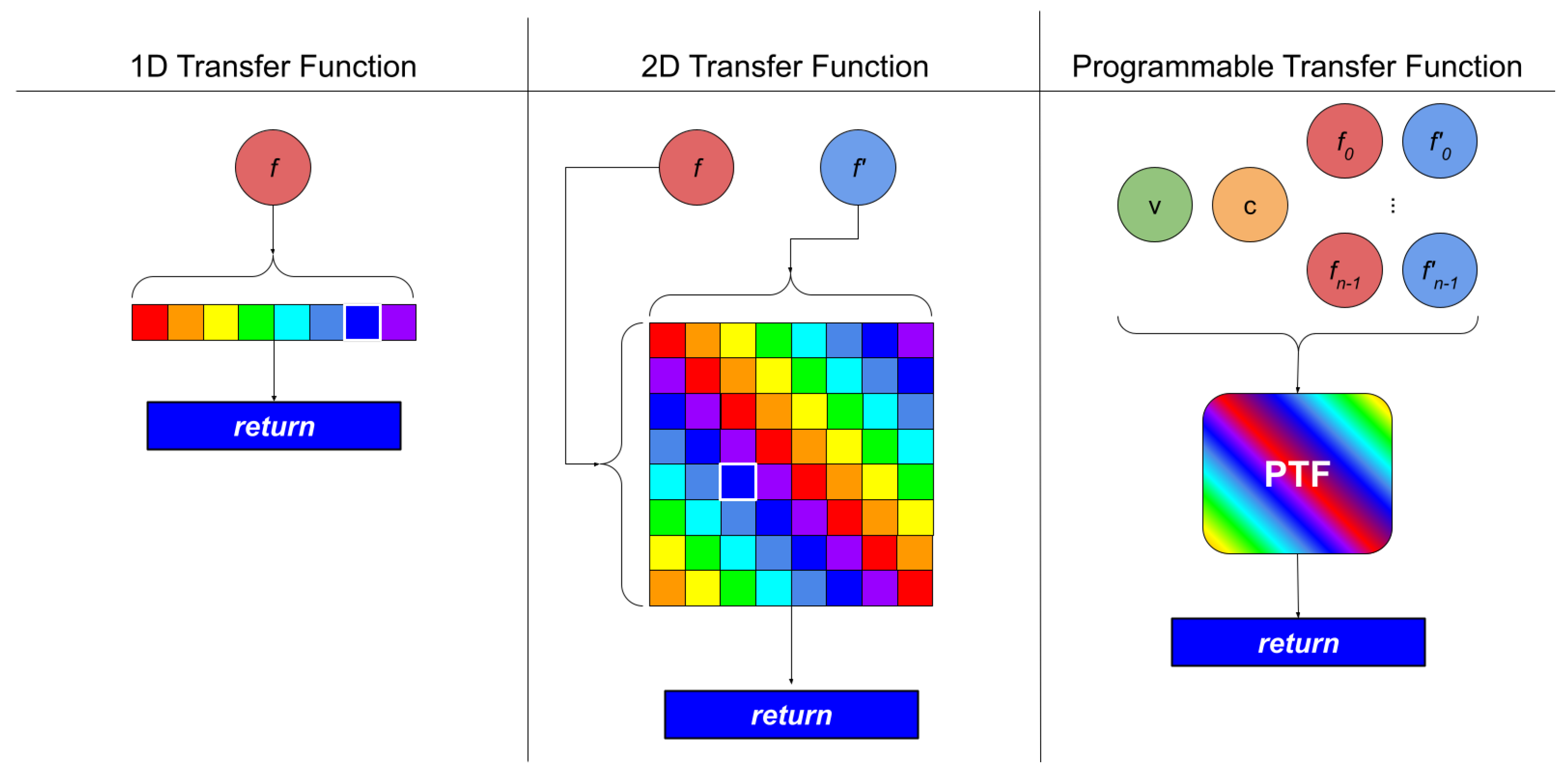
- Compact representation as succinct and fast shader code that alleviates the need for large arrays of slow lookups from memory; and
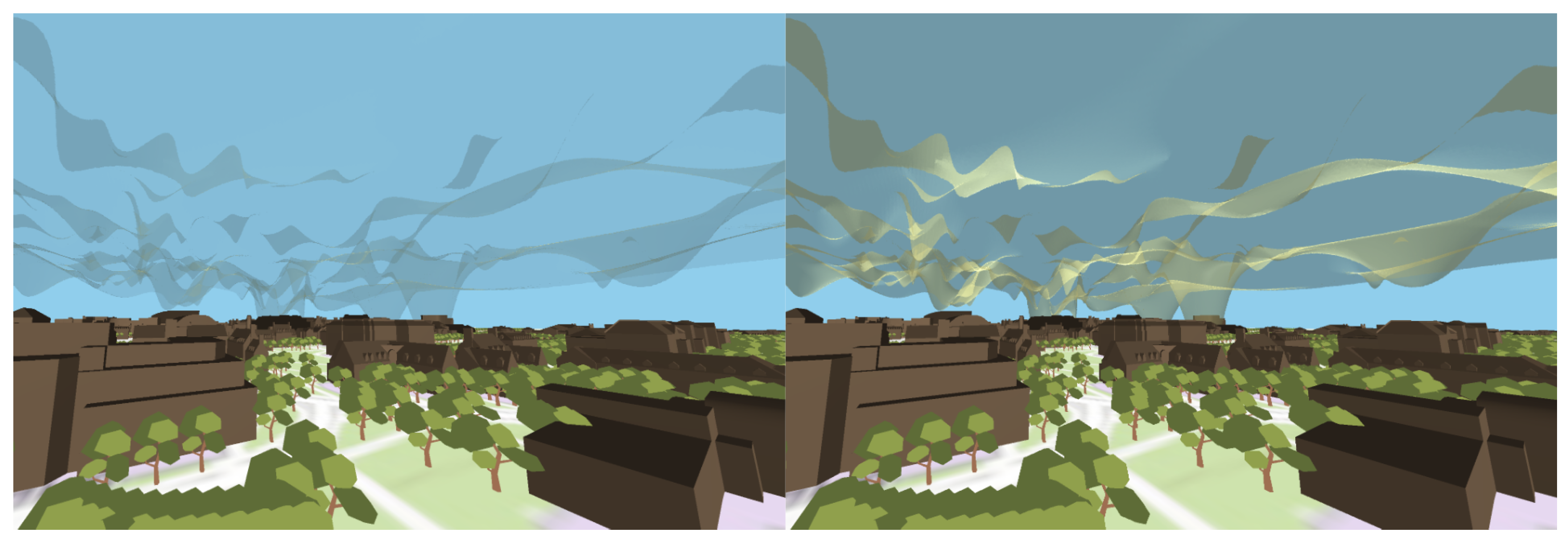
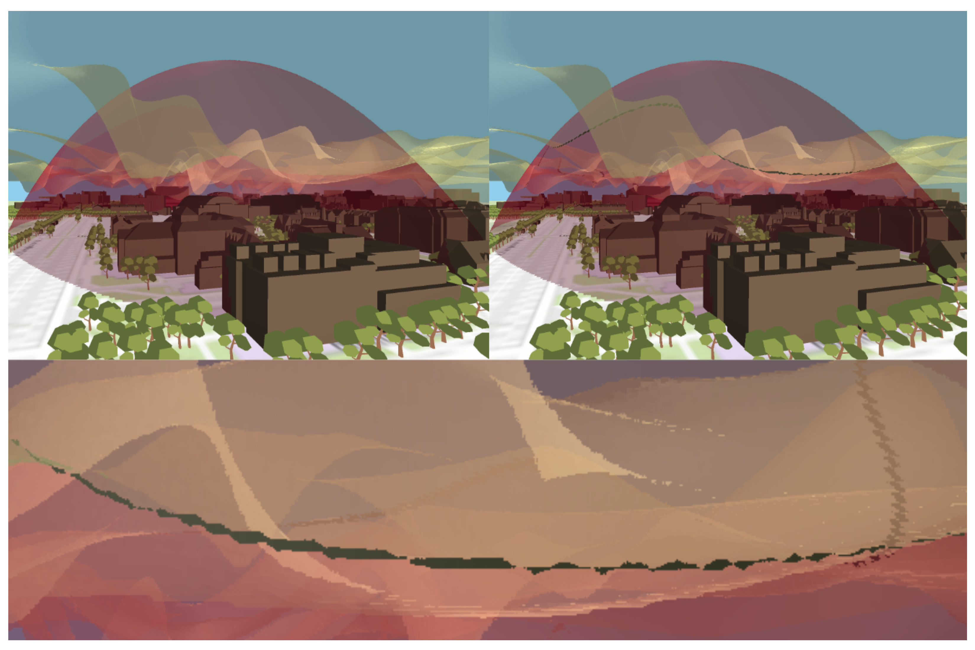
- Operation on multiple scalar fields and therefore can highlight features such as their intersection curves and regions.
2. Related Works
2.1. WiFi Data Visualization
2.2. Direct Volume Rendering
2.3. Interaction in Volume Rendering
2.4. Non-Photorealism
2.5. Multifield Data
3. Data
4. Programmable Transfer Functions
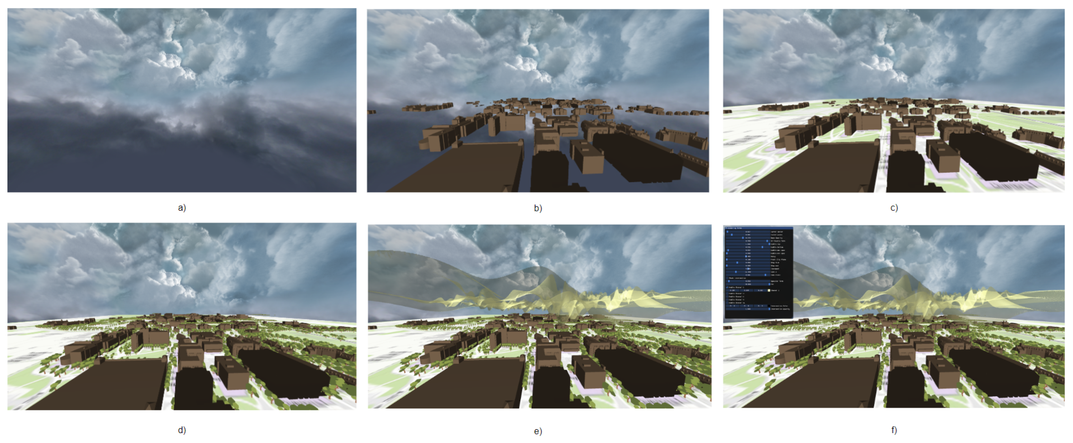
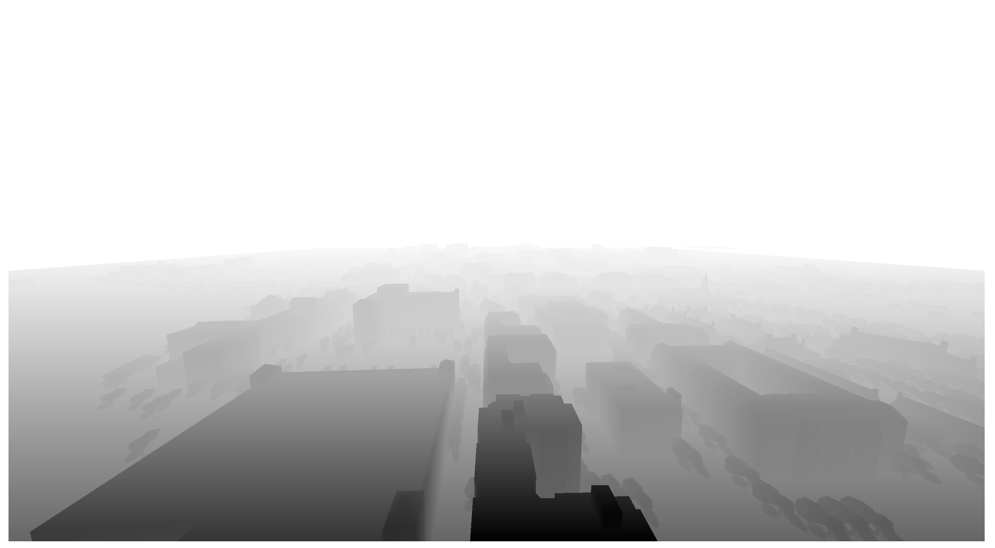
4.1. Base Direct Volume Rendering
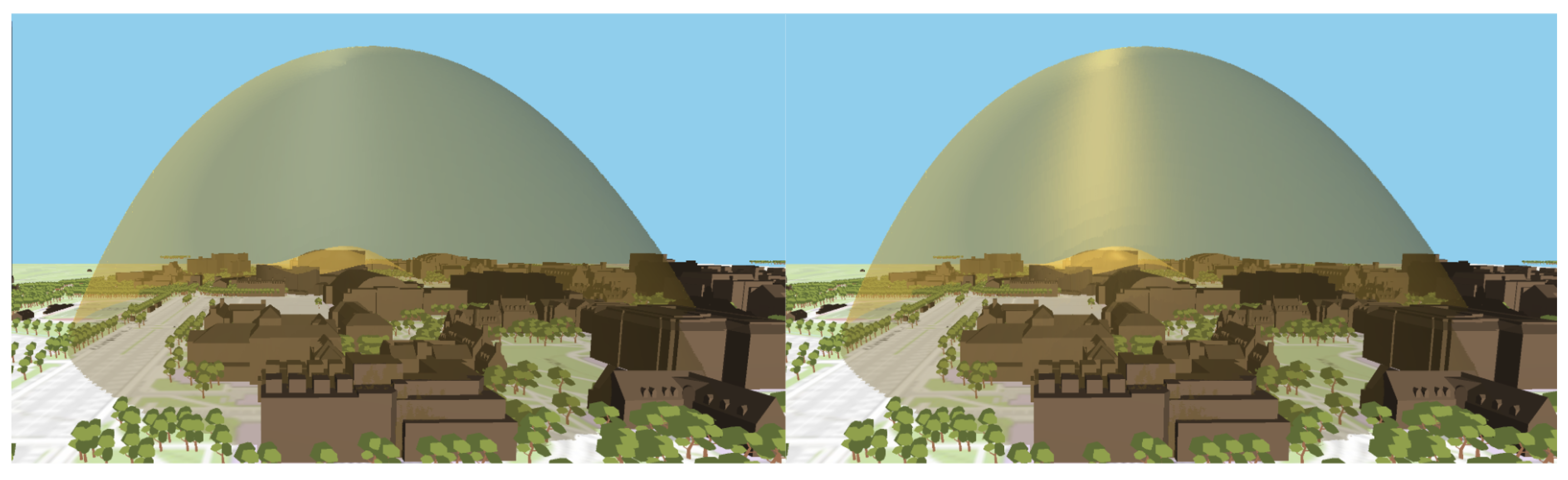
4.2. Silhouette Shading
| Algorithm 1 Silhouette Shading |
|
4.3. Specular Highlight Augmentation
| Algorithm 2 Specular Highlight Augmentation |
|
4.4. Multi-Volume Interaction
4.5. Performance
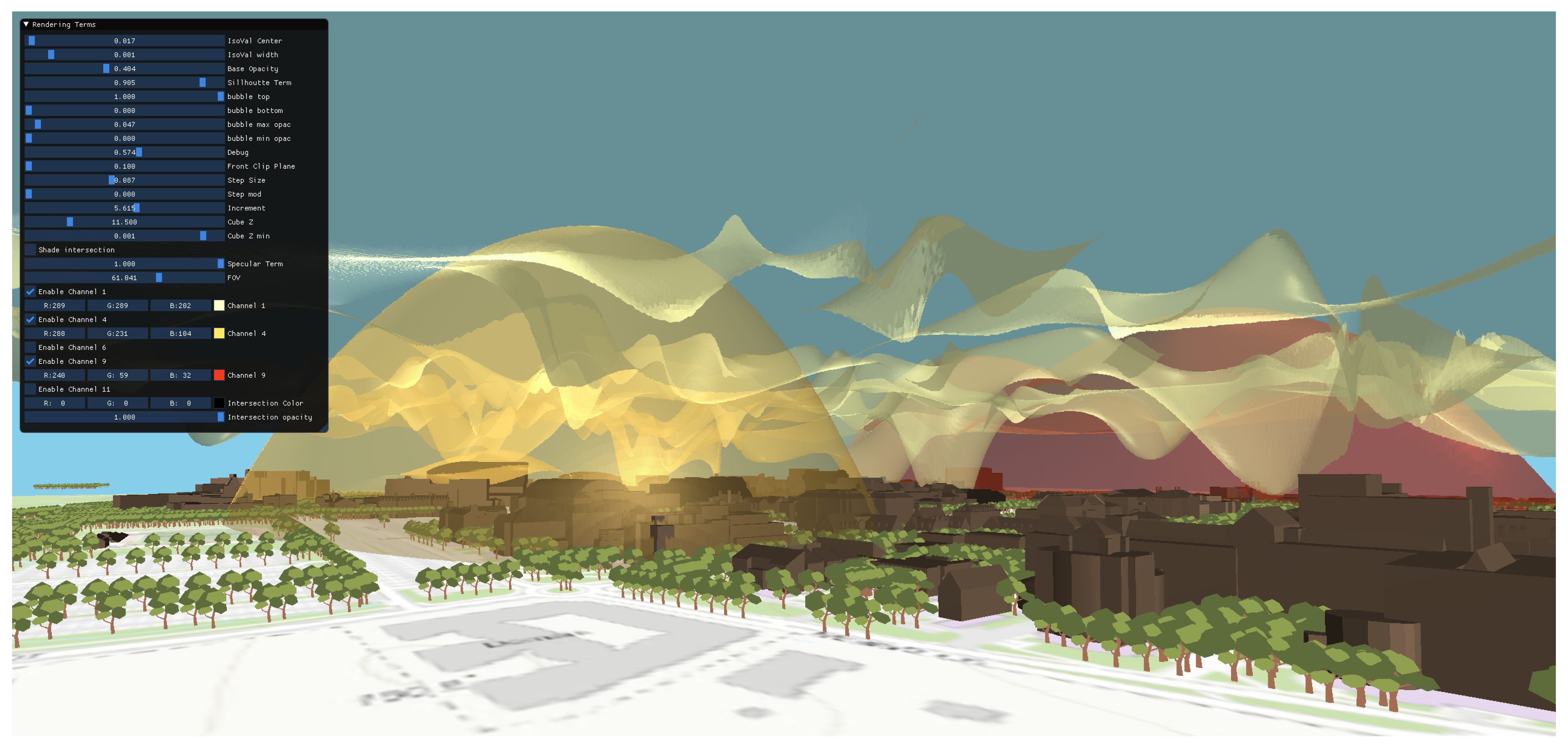
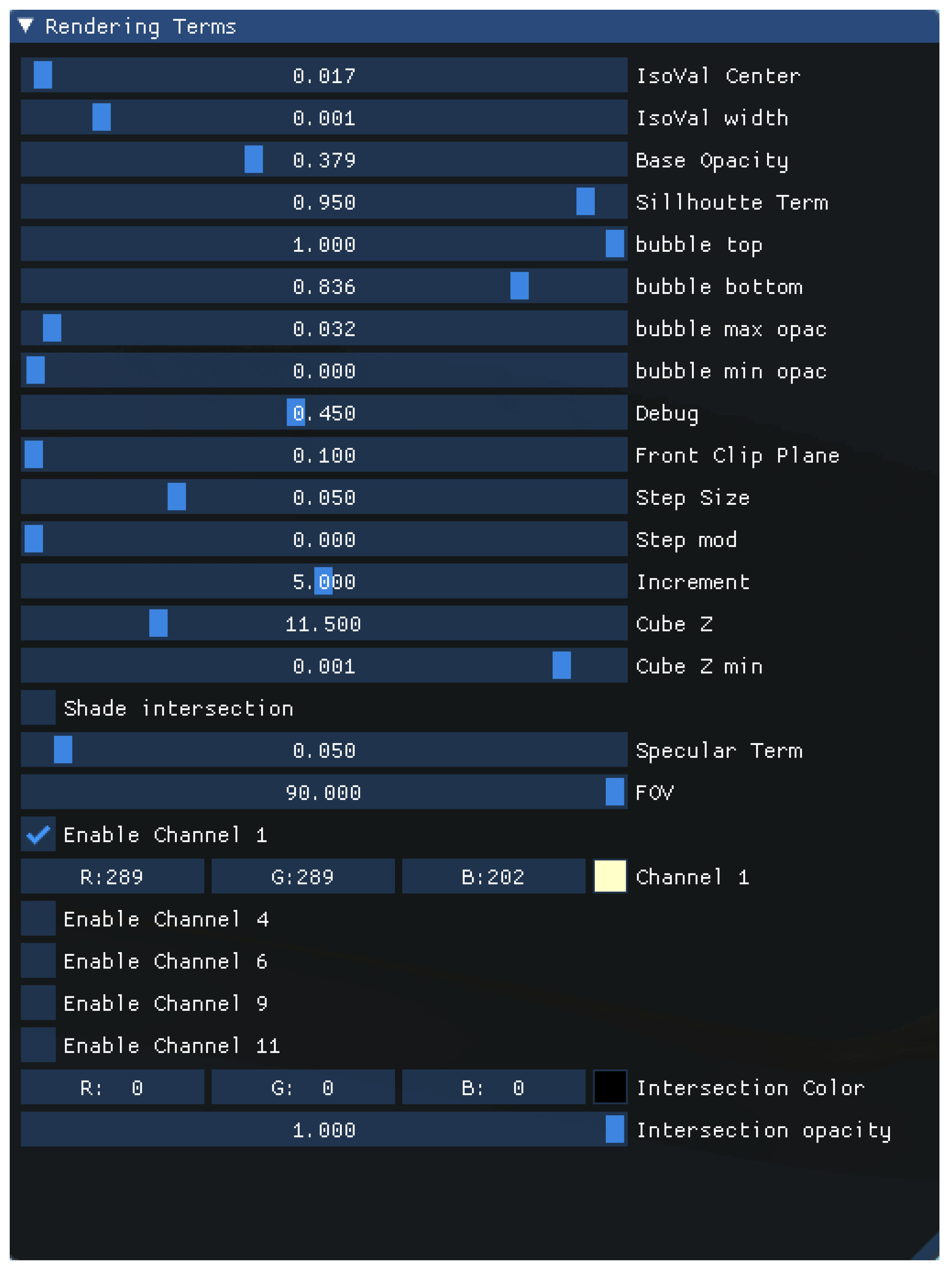
4.6. Interaction
5. Limitations and Future Work
5.1. Customized Rendering
5.2. Data Analytics
5.3. Visual Enhancements
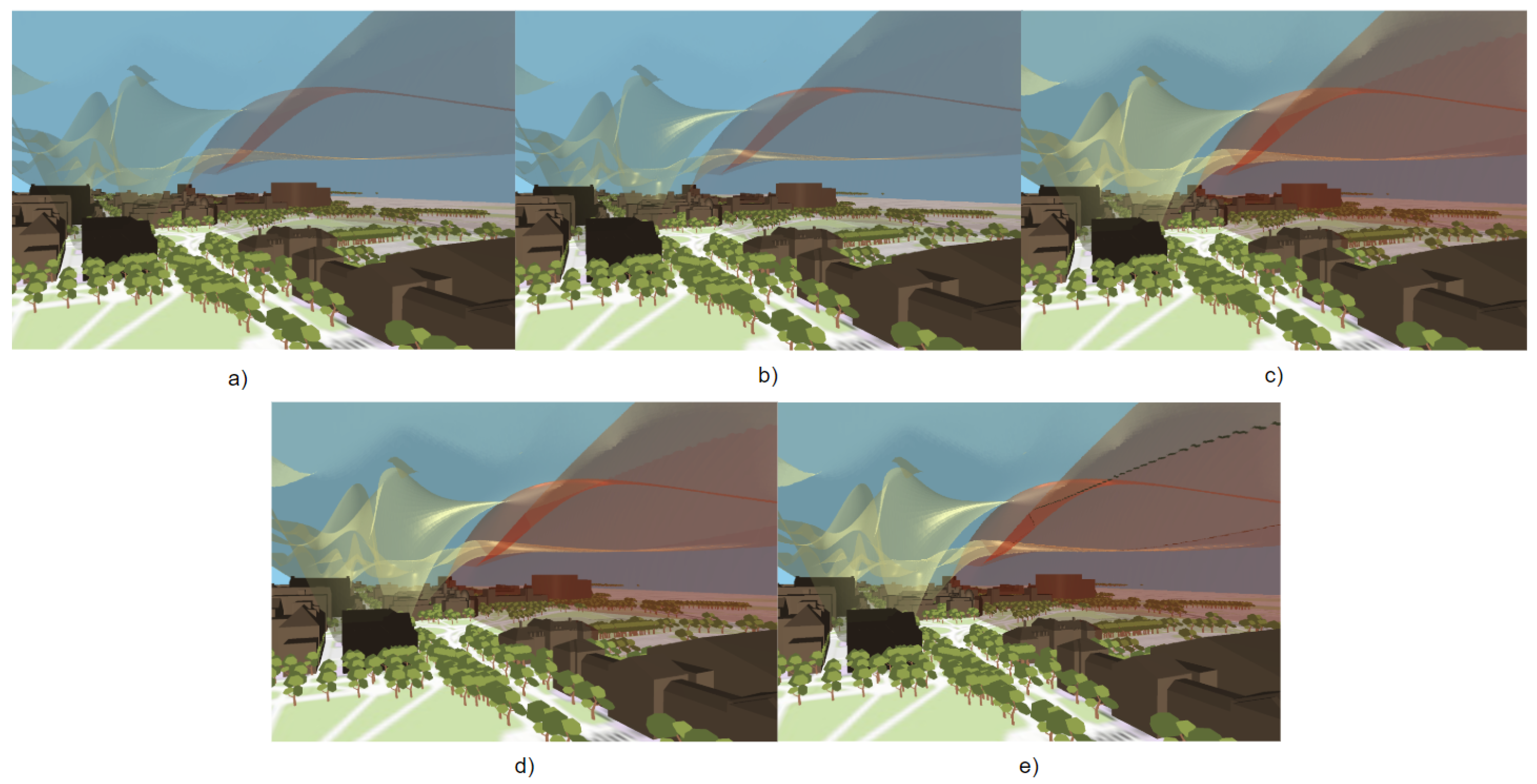
5.4. Multivolume Tools
| Algorithm 3 Multivolume Intersection Shading |
|
6. Conclusions
Author Contributions
Funding
Institutional Review Board Statement
Informed Consent Statement
Data Availability Statement
Conflicts of Interest
Abbreviations
| PTF | Programmable Transfer Functions |
| CSV | Comma-Separated File |
| WLAN | Wide Local Area Network |
| SSID | Service Set Identifier |
| BSSID | Basic Service Set Identifier |
| MAC | Media Access Control |
| GPS | Global Positioning Systems |
| RF | Radio Frequency |
| dBm | Decibel-milliwatts |
| CT | Computed Tomography |
| MRI | Magnetic Resonance Imaging |
| RAM | Random Access Memory |
| FPS | Frames Per Second |
| GUI | Graphical User Interface |
| CPU | Central Processing Unit |
References
- Kokkinos, V.; Stamos, K.; Kanakis, N.; Baumann, K.; Wilson, A.; Healy, J. Wireless crowdsourced performance monitoring and verification: WiFi performance measurement using end-user mobile device feedback. In Proceedings of the 2016 8th International Congress on Ultra Modern Telecommunications and Control Systems and Workshops (ICUMT), Lisbon, Portugal, 18–20 October 2016; pp. 432–437. [Google Scholar] [CrossRef]
- Sangkusolwong, W.; Apavatirut, A. Indoor WIFI Signal Prediction Using Modelized Heatmap Generator Tool. In Proceedings of the 2017 21st International Computer Science and Engineering Conference (ICSEC), Bangkok, Thailand, 15–18 November 2017; pp. 1–5. [Google Scholar] [CrossRef]
- Radu, V.; Kriara, L.; Marina, M.K. Pazl: A mobile crowdsensing based indoor WiFi monitoring system. In Proceedings of the 9th International Conference on Network and Service Management (CNSM 2013), Zurich, Switzerland, 14–18 October 2013; pp. 75–963. [Google Scholar] [CrossRef] [Green Version]
- Prentow, T.S.; Ruiz-Ruiz, A.J.; Blunck, H.; Stisen, A.; Kjærgaard, M.B. Spatio-temporal facility utilization analysis from exhaustive WiFi monitoring. Pervasive Mob. Comput. 2015, 16, 305–316. [Google Scholar] [CrossRef] [Green Version]
- Tervonen, J.; Hartikainen, M.; Heikkila, M.; Koskela, M. Applying and Comparing Two Measurement Approaches for the Estimation of Indoor WiFi Coverage. In Proceedings of the 2016 8th IFIP International Conference on New Technologies, Mobility and Security (NTMS), Larnaca, Cyprus, 21–23 November 2016; pp. 1–4. [Google Scholar] [CrossRef] [Green Version]
- Selamat, A.; Fujita, H.; Haron, H. New Trends in Software Methodologies, Tools and Techniques: Proceedings of the Thirteenth SoMeT_14; Google-Books-ID: oN3YBAAAQBAJ; IOS Press: Amsterdam, The Netherlands, 2014. [Google Scholar]
- Hu, H.; Myers, S.; Colizza, V.; Vespignani, A. WiFi networks and malware epidemiology. Proc. Natl. Acad. Sci. USA 2009, 106, 1318–1323. [Google Scholar] [CrossRef] [PubMed] [Green Version]
- Levoy, M. Display of surfaces from volume data. IEEE Comput. Graph. Appl. 1988, 8, 29–37. [Google Scholar] [CrossRef] [Green Version]
- Drebin, R.A.; Carpenter, L.; Hanrahan, P. Volume rendering. ACM Siggraph Comput. Graph. 1988, 22, 65–74. [Google Scholar] [CrossRef]
- Li, W.; Mueller, K.; Kaufman, A. Empty space skipping and occlusion clipping for texture-based volume rendering. In Proceedings of the IEEE Visualization, VIS 2003, Seattle, WA, USA, 19–24 October 2003; pp. 317–324. [Google Scholar] [CrossRef]
- He, T.; Hong, L.; Kaufman, A.; Pfister, H. Generation of Transfer Functions with Stochastic Search Techniques; IEEE Computer Society Press: Los Alamitos, CA, USA, 1996. [Google Scholar] [CrossRef] [Green Version]
- Kruger, J.; Westermann, R. Acceleration Techniques for GPU-based Volume Rendering. In Proceedings of the IEEE Visualization, VIS 2003, Seattle, WA, USA, 19–24 October 2003. [Google Scholar]
- LaMar, E.; Hamann, B.; Joy, K. Multiresolution techniques for interactive texture-based volume visualization. In Proceedings of the Visualization’99 (Cat. No.99CB37067), San Francisco, CA, USA, 24–29 October 1999; pp. 355–543. [Google Scholar] [CrossRef] [Green Version]
- Roettger, S.; Guthe, S.; Weiskopf, D.; Ertl, T.; Strasser, W. Smart Hardware-Accelerated Volume Rendering. In Proceedings of the VisSym03 Joint Eurographics-EEE TCVG Symposium on Visualization, Grenoble, France, 26–28 May 2003; p. 8. [Google Scholar] [CrossRef]
- Bista, S.; Zhuo, J.; Gullapalli, R.P.; Varshney, A. Visual Knowledge Discovery for Diffusion Kurtosis Datasets of the Human Brain. In Visualization and Processing of Higher Order Descriptors for Multi-Valued Data; Hotz, I., Schultz, T., Eds.; Springer International Publishing: Cham, Switzerland, 2015; pp. 213–234. [Google Scholar] [CrossRef]
- Cheng, H.C.; Cardone, A.; Jain, S.; Krokos, E.; Narayan, K.; Subramaniam, S.; Varshney, A. Deep-Learning-Assisted Volume Visualization. IEEE Trans. Vis. Comput. Graph. 2019, 25, 1378–1391. [Google Scholar] [CrossRef] [PubMed]
- Sharma, O.; Arora, T.; Khattar, A. Graph-Based Transfer Function for Volume Rendering. Comput. Graph. Forum 2020, 39, 76–88. [Google Scholar] [CrossRef]
- Pflesser, B.; Tiede, U.; Höhne, K.H. Towards Realistic Visualization for Surgery Rehearsal. In Computer Vision, Virtual Reality and Robotics in Medicine; Ayache, N., Ed.; Lecture Notes in Computer Science; Springer: Berlin/Heidelberg, Germany, 1995; pp. 487–491. [Google Scholar] [CrossRef]
- Carpendale, M.S.T.; Cowperthwaite, D.; Fracchia, F. Distortion viewing techniques for 3-dimensional data. In Proceedings of the IEEE Symposium on Information Visualization’96, San Francisco, CA, USA, 28–29 October 1996; pp. 46–53. [Google Scholar] [CrossRef]
- Ip, C.Y.; Varshney, A.; JaJa, J. Hierarchical Exploration of Volumes Using Multilevel Segmentation of the Intensity-Gradient Histograms. IEEE Trans. Vis. Comput. Graph. 2012, 18, 2355–2363. [Google Scholar] [CrossRef] [PubMed] [Green Version]
- Kniss, J.; Kindlmann, G.; Hansen, C. Multidimensional transfer functions for interactive volume rendering. IEEE Trans. Vis. Comput. Graph. 2002, 8, 270–285. [Google Scholar] [CrossRef]
- Viola, I.; Kanitsar, A.; Groller, M. Importance-driven volume rendering. IEEE Vis. 2004, 2004, 139–145. [Google Scholar] [CrossRef]
- Treavett, S.; Chen, M. Pen-and-ink rendering in volume visualisation. In Proceedings of the Visualization, VIS 2000, (Cat. No.00CH37145), Salt Lake City, UT, USA, 8–13 October 2000; pp. 203–210. [Google Scholar] [CrossRef]
- Csébfalvi, B.; Mroz, L.; Hauser, H.; König, A.; Gröller, E. Fast Visualization of Object Contours by Non-Photorealistic Volume Rendering. Comput. Graph. Forum 2001, 20, 452–460. [Google Scholar] [CrossRef]
- Linsen, L.; Van Long, T.; Rosenthal, P.; Rosswog, S. Surface Extraction from Multi-field Particle Volume Data Using Multi-dimensional Cluster Visualization. IEEE Trans. Vis. Comput. Graph. 2008, 14, 1483–1490. [Google Scholar] [CrossRef] [PubMed]
- Kniss, J.; Hansen, C. Volume Rendering Multivariate Data to Visualize Meteorological Simulations: A Case Study; The Eurographics Association: Munich, Germany, 2002. [Google Scholar]
- Kniss, J.; premoze, S.; Ikits, M.; Lefohn, A.; Hansen, C.; Praun, E. Gaussian transfer functions for multi-field volume visualization. In Proceedings of the IEEE Visualization, VIS 2003, Seattle, WA, USA, 19–24 October 2003; pp. 497–504. [Google Scholar] [CrossRef] [Green Version]
- Jang, Y.; Botchen, R.P.; Lauser, A.; Ebert, D.S.; Gaither, K.P.; Ertl, T. Enhancing the Interactive Visualization of Procedurally Encoded Multifield Data with Ellipsoidal Basis Functions. Comput. Graph. Forum 2006, 25, 587–596. [Google Scholar] [CrossRef]
- Sauber, N.; Theisel, H.; Seidel, H.P. Multifield-Graphs: An Approach to Visualizing Correlations in Multifield Scalar Data. IEEE Trans. Vis. Comput. Graph. 2006, 12, 917–924. [Google Scholar] [CrossRef] [PubMed] [Green Version]
- Demir, I.; Kehrer, J.; Westermann, R. Screen-space silhouettes for visualizing ensembles of 3D isosurfaces. In Proceedings of the 2016 IEEE Pacific Visualization Symposium (PacificVis), Taipei, Taiwan, 19–22 April 2016; pp. 204–208. [Google Scholar] [CrossRef]
- Fernando, R. GPU Gems: Programming Techniques, Tips and Tricks for Real-Time Graphics; Pearson Higher Education: San Francisco, CA, USA, 2004; Chapter 39. [Google Scholar]
- Jankowai, J.; Hotz, I. Feature Level-Sets: Generalizing Iso-Surfaces to Multi-Variate Data. IEEE Trans. Vis. Comput. Graph. 2020, 26, 1308–1319. [Google Scholar] [CrossRef] [PubMed] [Green Version]


| Base | Specular | Silhouette | Spec + Silh | Intersection | All 3 | |
|---|---|---|---|---|---|---|
| 1 Volume (interior) | 105 | 105 | 105 | 105 | NA | NA |
| 1 Volume (exterior) | 181 | 181 | 181 | 181 | NA | NA |
| 5 Volumes (interior) | 85 | 85 | 85 | 85 | 85 | 85 |
| 5 Volumes (exterior) | 116 | 116 | 116 | 116 | 116 | 116 |
Publisher’s Note: MDPI stays neutral with regard to jurisdictional claims in published maps and institutional affiliations. |
© 2022 by the authors. Licensee MDPI, Basel, Switzerland. This article is an open access article distributed under the terms and conditions of the Creative Commons Attribution (CC BY) license (https://creativecommons.org/licenses/by/4.0/).
Share and Cite
Rowden, A.; Krokos, E.; Whitley, K.; Varshney, A. Visualization of WiFi Signals Using Programmable Transfer Functions. Information 2022, 13, 224. https://doi.org/10.3390/info13050224
Rowden A, Krokos E, Whitley K, Varshney A. Visualization of WiFi Signals Using Programmable Transfer Functions. Information. 2022; 13(5):224. https://doi.org/10.3390/info13050224
Chicago/Turabian StyleRowden, Alexander, Eric Krokos, Kirsten Whitley, and Amitabh Varshney. 2022. "Visualization of WiFi Signals Using Programmable Transfer Functions" Information 13, no. 5: 224. https://doi.org/10.3390/info13050224
APA StyleRowden, A., Krokos, E., Whitley, K., & Varshney, A. (2022). Visualization of WiFi Signals Using Programmable Transfer Functions. Information, 13(5), 224. https://doi.org/10.3390/info13050224