
A Dynamic Convolutional Network-Based Model for Knowledge Graph Completion


Abstract
:1. Introduction
- We propose a new model, called DyConvNE, based on a dynamic convolution network, which uses dynamic convolution to dynamically assign weights to the interaction features of the extracted entities and relationship embeddings;
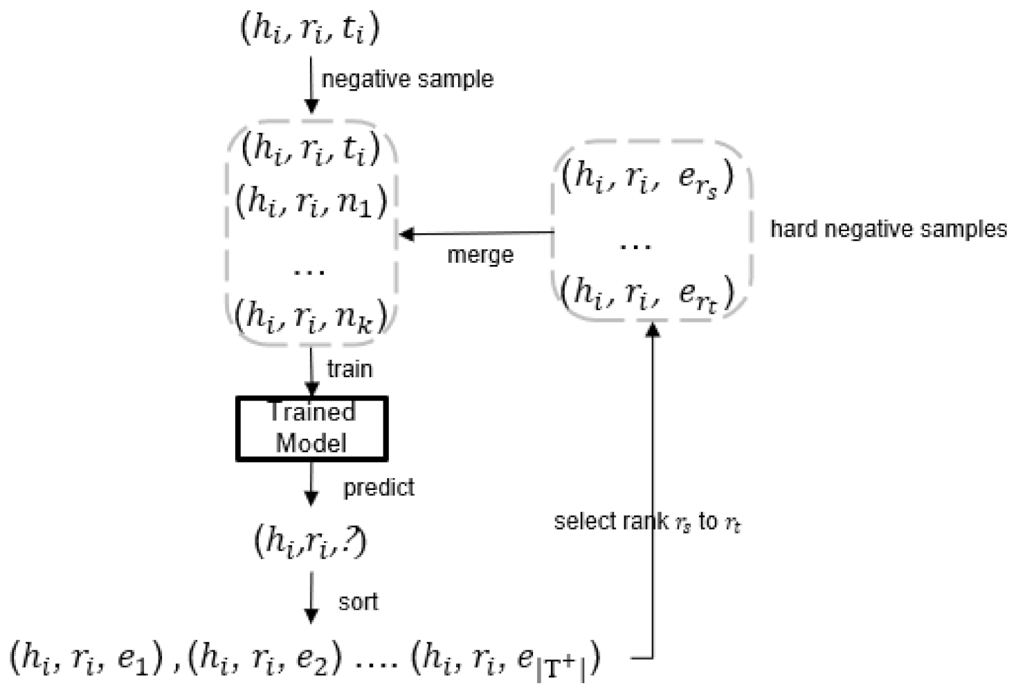
- We propose a method to mine hard negative samples and demonstrate the effectiveness of the method through ablation experiments;
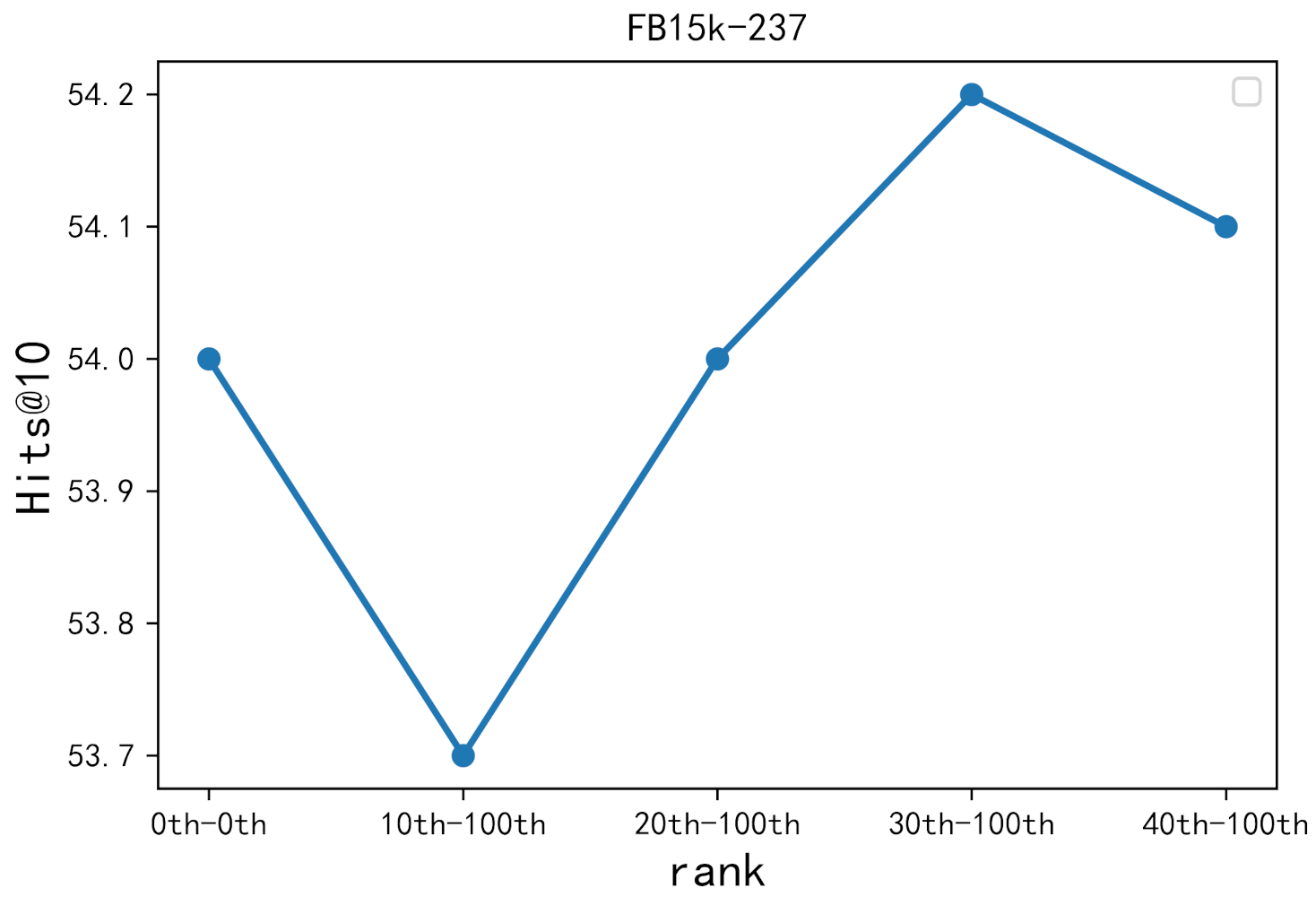
- We use specific-relationship-testing to obtain better performance on Hits@1;
- We conduct some experiments to evaluate the performance of the proposed method. Experimental results demonstrate that our method obtains competitive performance on both WN18RR and FB15k-237.
2. Related Work
3. Our Approach
3.1. Definition
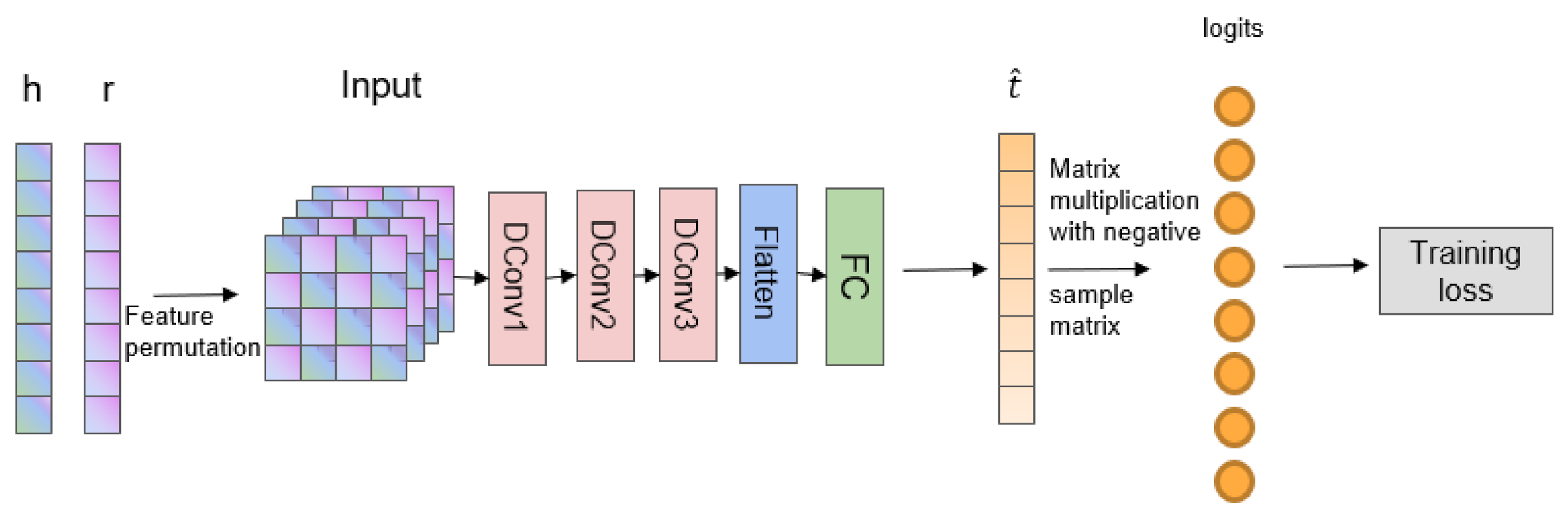
3.2. Our Model
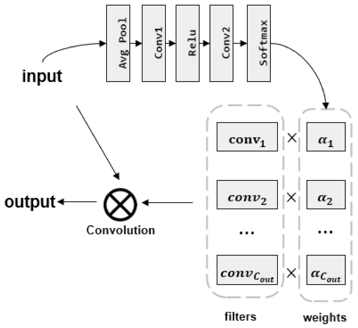
3.3. Dynamic Convolution
3.4. Mining Hard Negative Samples
3.5. Training Objective
4. Experiments
4.1. Datasets
4.2. Experimental Setup
4.3. Main Results
4.4. Specific Relationship Testing
4.5. Case Study
4.6. Ablation Study
4.7. Hard Negative Sampling Study
5. Conclusions
Author Contributions
Funding
Data Availability Statement
Conflicts of Interest
References
- Huang, X.; Zhang, J.; Li, D.; Li, P. Knowledge graph embedding based question answering. In Proceedings of the 12th ACM International Conference on Web Search and Data Mining, Melbourne, Australia, 11–15 February 2019; pp. 105–113. [Google Scholar]
- He, H.; Balakrishnan, A.; Eric, M.; Liang, P. Learning symmetric collaborative dialogue agents with dynamic knowledge graph embeddings. In Proceedings of the 55th Annual Meeting of the Association for Computational Linguistics, Vancouver, BC, Canada, 30 July–4 August 2017; pp. 1767–1776. [Google Scholar]
- Madotto, A.; Wu, C.; Fung, P. Mem2seq: Effectively incorporating knowledge bases into end-to-end task-oriented dialog systems. In Proceedings of the 56th Annual Meeting of the Association for Computational Linguistics, Melbourne, Australia, 15–20 July 2018; pp. 1468–1478. [Google Scholar]
- Zhang, F.; Yuan, N.; Nicholas, J.; Lian, D.; Xie, X.; Ma, W. Collaborative knowledge base embedding for recommender systems. In Proceedings of the 22nd ACM SIGKDD international conference on knowledge discovery and data mining, San Francisco, CA, USA, 13–17 August 2016; pp. 353–362. [Google Scholar]
- Chen, X.; Jia, S.; Xiang, Y. A review: Knowledge reasoning over knowledge graph. Expert Syst. Appl. 2020, 141, 112948. [Google Scholar] [CrossRef]
- Bollacker, K.; Evans, C.; Paritosh, P.; Sturge, T.; Taylor, J. Freebase: A collaboratively created graph database for structuring human knowledge. In Proceedings of the 2008 ACM SIGMOD International Conference on Management of Data, Vancouver, BC, Canada, 9–12 June 2008; pp. 1247–1250. [Google Scholar]
- Vrandečić, D.; Krötzsch, M. Wikidata: A free collaborative knowledgebase. Commun. ACM 2014, 57, 78–85. [Google Scholar] [CrossRef]
- Lehmann, J.; Isele, R.; Jakob, M.; Jentzsch, A.; Kontokostas, D.; Mendes, P.; Hellmann, S.; Morsey, M.; van Kleef, P.; Auer, S. Dbpedia—A large-scale, multilingual knowledge base extracted from wikipedia. Semant. Web J. 2015, 6, 167–195. [Google Scholar] [CrossRef] [Green Version]
- Ji, S.; Pan, S.; Cambria, E.; Marttinen, P.; Philip, S. A survey on knowledge graphs: Representation, acquisition, and applications. IEEE Trans. Neural Netw. Learn. Syst. 2021, 33, 494–514. [Google Scholar] [CrossRef] [PubMed]
- Dai, Y.; Wang, S.; Xiong, N.N.; Guo, W. A survey on knowledge graph embedding: Approaches, applications and benchmarks. Electronics 2020, 9, 750. [Google Scholar] [CrossRef]
- Vashishth, S.; Sanyal, S.; Nitin, V.; Agrawal, N.; Talukdar, P.P. InteractE: Improving Convolution-Based Knowledge Graph Embeddings by Increasing Feature Interactions. In Proceedings of the AAAI Conference on Artificial Intelligence, New York, NY, USA, 7–12 February 2020; AAAI Press: Palo Alto, CA, USA, 2020; pp. 3009–3016. [Google Scholar]
- Dettmers, T.; Minervini, P.; Stenetorp, P.; Riedel, S. Convolutional 2d knowledge graph embeddings. In Proceedings of the AAAI Conference on Artificial Intelligence, Palo Alto, CA, USA, 4–9 February 2017; AAAI Press: Palo Alto, CA, USA, 2017; pp. 1811–1818. [Google Scholar]
- Chen, Y.; Dai, X.; Liu, M.; Chen, D.; Yuan, L.; Liu, Z. Dynamic convolution: Attention over convolution kernels. In Proceedings of the IEEE/CVF Conference on Computer Vision and Pattern Recognition, Salt Lake City, UT, USA, 18–23 June 2020; pp. 11030–11039. [Google Scholar]
- Rossi, A.; Barbosa, D.; Firmani, D.; Matinata, A.; Merialdo, P. Knowledge graph embedding for link prediction: A comparative analysis. ACM Trans. Knowl. Discov. Data TKDD 2021, 15, 1–49. [Google Scholar] [CrossRef]
- Wang, M.; Qiu, L.; Wang, X. A Survey on Knowledge Graph Embeddings for Link Prediction. Symmetry 2021, 13, 485. [Google Scholar] [CrossRef]
- Nickel, M.; Tresp, V.; Kriegel, H.P. A Three-Way Model for Collective Learning on Multi-Relational Data. In Proceedings of the ICML, Washington, DC, USA, 28 June–2 July 2011; pp. 809–816. [Google Scholar]
- Socher, R.; Chen, D.; Manning, C.; Ng, A. Reasoning with Neural Tensor Networks for Knowledge Base Completion; MIT Press: Cambridge, MA, USA, 2013; pp. 926–934. [Google Scholar]
- Nickel, M.; Rosasco, L.; Poggio, T.A. Holographic Embeddings of Knowledge Graphs. In Proceedings of the AAAI Conference on Artificial Intelligence, Phoenix, AZ, USA, 12–17 February 2016; AAAI: Phoenix, AZ, USA, 2016; pp. 1955–1961. [Google Scholar]
- Bordes, A.; Usunier, N.; Garcia-Duran, A.; Weston, J.; Yakhnenko, O. Translating embeddings for modeling multi-relational data. Adv. Neural Inf. Process. 2013, 26, 2787–2795. [Google Scholar]
- Yang, B.; Yih, W.; He, X.; Gao, J.; Deng, L. Embedding entities and relations for learning and inference in knowledge bases. In Proceedings of the ICLR (Poster), San Diego, CA, USA, 7–9 May 2015. [Google Scholar]
- Trouillon, T.; Welbl, J.; Riedel, S.; Gaussier, É.; Bouchard, G. Complex embeddings for simple link prediction. In Proceedings of the International Conference on Machine Learning, New York, NY, USA, 20–22 June 2016; ICML: New York City, NY, USA, 2016; pp. 2071–2080. [Google Scholar]
- Nguyen, D.Q.; Nguyen, T.D.; Nguyen, D.Q.; Phung, D.Q. A novel embedding model for knowledge base completion based on convolutional neural network. In Proceedings of the NAACL-HLT, New Orleans, LA, USA, 1–6 June 2018; pp. 327–333. [Google Scholar]
- Xavier, G.; Antoine, B.; Yoshua, B. Deep sparse rectifier neural networks. In Proceedings of the AISTATS, Lauderdale, FL, USA, 11–13 April 2011; pp. 315–323. [Google Scholar]
- Jie, H.; Li, S.; Gang, S. Squeeze-and-excitation networks. In Proceedings of the IEEE Conference on Computer Vision and Pattern Recognition (CVPR), Salt Lake City, UT, USA, 18–22 June 2018; pp. 7132–7141. [Google Scholar]
- Kingma, D.; Ba, J. Adam: A method for stochastic optimization. arXiv 2014, arXiv:1412.6980. [Google Scholar]
- Toutanova, K.; Chen, D.; Pantel, P.; Poon, H.; Choudhury, P.; Gamon, M. Representing Text for Joint Embedding of Text and Knowledge Bases. In Proceedings of the 2015 Conference on Empirical Methods in Natural Language Processing, Lisbon, Portugal, 17–21 September 2015; pp. 1499–1509. [Google Scholar]
- Oh, B.; Seo, S.; Lee, L. Knowledge graph completion by context-aware convolutional learning with multi-hop neighborhoods. In Proceedings of the 27th ACM International Conference on Information and Knowledge Management, Torino, Italy, 22–26 October 2018; pp. 257–266. [Google Scholar]
- Shang, C.; Tang, Y.; Huang, J.; Bi, J.; He, X.; Zhou, B. End-to-End Structure-Aware Convolutional Networks for Knowledge Base Completion. In Proceedings of the AAAI Conference on Artificial Intelligence, Honolulu, HI, USA, 27 January–1 February 2019; AAAI Press: Palo Alto, CA, USA, 2019; pp. 3060–3067. [Google Scholar]


| Layer | Size of Stride | Number of Filters | Size of Kernel | Size of Padding | Output Size |
|---|---|---|---|---|---|
| Input | - | - | - | - | 20 × 20 × 4 |
| DConv1 | 1 | 64 | 3 × 3 | 1 | 20 × 20 × 64 |
| DConv2 | 1 | 128 | 3 × 3 | 1 | 20 × 20 × 128 |
| DConv3 | 1 | 256 | 3 × 3 | 1 | 20 × 20 × 256 |
| Flatten | - | - | - | - | 102,400 |
| FC | - | - | - | - | 200 |
| Layer | Size of Stride | Number of Filters | Size of Kernel | Size of Padding | Output Size |
|---|---|---|---|---|---|
| Input | - | - | - | - | |
| Avg. Pool | - | - | - | - | |
| Conv1 | 1 | 1 × 1 | 0 | ||
| Relu | - | - | - | - | |
| Conv2 | 1 | 1 × 1 | 0 | 1 × 1 × | |
| Softmax | - | - | - | - | |
| Output | - | - | - | - |
| Parameter | Value | |
|---|---|---|
| FB15k-237 | WN18RR | |
| k | 1000 | 5000 |
| 30th | 20th | |
| 100th | 200th | |
| Dataset | Triples | ||||
|---|---|---|---|---|---|
| Train | Valid | Test | |||
| FB15k-237 | 14,541 | 237 | 272,115 | 17,535 | 20,466 |
| WN18RR | 40,943 | 11 | 86,835 | 3034 | 3134 |
| Parameter | Value | |
|---|---|---|
| FB15k-237 | WN18RR | |
| Learning rate | 0.001 | 0.001 |
| Epoch | 500 | 500 |
| Batch size | 128 | 256 |
| The dimensionality of embedding | 200 | 200 |
| Models | WN18RR | FB15k-237 | ||||||
|---|---|---|---|---|---|---|---|---|
| MR | MRR | Hits@1 | Hits@10 | MR | MRR | Hits@1 | Hits@10 | |
| TransE [19] | 2300 | 0.243 | 4.27 | 53.2 | 323 | 0.279 | 19.8 | 44.1 |
| DisMult [20] | 7000 | 0.444 | 41.2 | 50.4 | 512 | 0.281 | 19.9 | 44.6 |
| ComplEx [21] | 7882 | 0.449 | 40.9 | 53 | 546 | 0.278 | 19.4 | 45 |
| CACL [27] | 3154 | 0.472 | - | 54.3 | 235 | 0.349 | - | 48.7 |
| SACN [28] | - | 0.470 | 43.0 | 54.0 | - | 0.350 | 26.0 | 54.0 |
| ConvE [12] | 4464 | 0.456 | 41.9 | 53.1 | 245 | 0.312 | 22.5 | 49.7 |
| ConvKB [22] | 2554 | 0.248 | - | 52.5 | 257 | 0.396 | - | 51.7 |
| InteractE [11] | 5202 | 0.463 | 43.0 | 52.8 | 172 | 0.354 | 26.3 | 53.5 |
| DyConvNE (ours) | 4531 | 0.474 | 43.5 | 55.2 | 181 | 0.358 | 26.5 | 54.2 |
| Models | Wn18RR | FB15k-237 |
|---|---|---|
| Hits@1 | Hits@1 | |
| TransE [19] | 4.27 | 19.8 |
| DisMult [20] | 41.2 | 19.9 |
| ComplEx [21] | 40.9 | 19.4 |
| SACN [28] | 43.0 | 26.0 |
| ConvE [12] | 41.9 | 22.5 |
| InteractE [11] | 43.0 | 26.3 |
| DyConvNE | 43.5 | 26.5 |
| DyConvNe-SR | 46.3 | 28.4 |
| Query and Target | Top Predictions | |
|---|---|---|
| Traditional Testing Method | Specific-Relationship-Testing Method | |
| John A. Lasseter | Randy Newman | |
| Query: (Pixar Animation Studios, | Pete Docter | Mike Patton |
| artist, ?) | Andrew Stanton | Ziggy Marley |
| Target: Randy Newman | Randy Newman | AC/DC |
| Walt Disney Pictures | Blondie | |
| The Shubert Organization | Emanuel “Manny” Azenberg | |
| Query: (?, profession, | Emanuel “Manny” Azenberg | Marvin Neil Simon |
| theatrical producer) | Marvin Neil Simon | Tony Kushner |
| Target: Emanuel “Manny” Azenberg | Tony Kushner | Arthur Asher Miller |
| Arthur Asher Miller | John Patrick Shanley | |
| Models | FB15k-237 | WN18RR | ||||
|---|---|---|---|---|---|---|
| MR | MRR | Hits@10 | MR | MRR | Hits@10 | |
| DyConvNE-conv | 186 | 0.353 | 53.9 | 5455 | 0.44 | 51.6 |
| DyConvNE-dyconv | 185 | 0.356 | 54.0 | 4801 | 0.452 | 52.5 |
| DyConvNE-dyconv-neg | 181 | 0.358 | 54.2 | 4531 | 0.474 | 55.2 |
Publisher’s Note: MDPI stays neutral with regard to jurisdictional claims in published maps and institutional affiliations. |
© 2022 by the authors. Licensee MDPI, Basel, Switzerland. This article is an open access article distributed under the terms and conditions of the Creative Commons Attribution (CC BY) license (https://creativecommons.org/licenses/by/4.0/).
Share and Cite
Peng, H.; Wu, Y. A Dynamic Convolutional Network-Based Model for Knowledge Graph Completion. Information 2022, 13, 133. https://doi.org/10.3390/info13030133
Peng H, Wu Y. A Dynamic Convolutional Network-Based Model for Knowledge Graph Completion. Information. 2022; 13(3):133. https://doi.org/10.3390/info13030133
Chicago/Turabian StylePeng, Haoliang, and Yue Wu. 2022. "A Dynamic Convolutional Network-Based Model for Knowledge Graph Completion" Information 13, no. 3: 133. https://doi.org/10.3390/info13030133
APA StylePeng, H., & Wu, Y. (2022). A Dynamic Convolutional Network-Based Model for Knowledge Graph Completion. Information, 13(3), 133. https://doi.org/10.3390/info13030133