Abstract
In this paper, we propose a method that uses low-resolution infrared (IR) array sensors to identify the presence and location of people indoors. In the first step, we introduce a method that uses 32 × 24 pixels IR array sensors and relies on deep learning to detect the presence and location of up to three people with an accuracy reaching 97.84%. The approach detects the presence of a single person with an accuracy equal to 100%. In the second step, we use lower end IR array sensors with even lower resolution (16 × 12 and 8 × 6) to perform the same tasks. We invoke super resolution and denoising techniques to faithfully upscale the low-resolution images into higher resolution ones. We then perform classification tasks and identify the number of people and their locations. Our experiments show that it is possible to detect up to three people and a single person with accuracy equal to 94.90 and 99.85%, respectively, when using frames of size 16 × 12. For frames of size 8 × 6, the accuracy reaches 86.79 and 97.59%, respectively. Compared to a much complex network (i.e., RetinaNet), our method presents an improvement of over 8% in detection.
1. Introduction
With the advances in the field of medicine and healthcare [1,2], a trend has been observed in almost all countries: societies are becoming older, and the ratio of people over 65 years old is becoming higher [3,4,5]. For instance, the median ages in Japan, France and Germany are 47.3, 41 and 47.1 years, respectively. Nevertheless, people over 65 in in these countries represent 28.40, 20.75 and 21.69% of their respective total populations (https://www.worldometers.info/demographics/. Accessed 12 January 2022). This increase in terms of median age and percentage of elderly people makes it necessary to find a way to continuously monitor these people, in particular, ones living alone [6]. This is because they are more vulnerable and subject to severe accidents that might occur and that need immediate intervention to help them. Chances of these people facing such severe accidents such as falling are quite high. The World Health Organization [7] reported that between 28 and 35% of elderly people fall at least once every year. Some of these falls are very harmful and might even be lethal. Therefore, it is fair to affirm that monitoring elderly people living alone is one of the biggest concerns in the field of healthcare. The technological advances and the “revolution” of Internet of Things (IoT) are very promising to automate a great part of this monitoring process. They would allow to build autonomous systems that allow for immediate detection of accidents. Such systems would monitor a variety of aspects related to patients including monitoring vital signals (e.g., pulse, heartbeat and respiration rates, etc.) [8,9], the detection of activities [10,11], in particular, the detection of fall activities [12], etc.
A key step toward building such a system is the identification of the presence of the person under monitoring and determining their location at any moment. This is because, in most of the state-of-the-art works, monitoring vital signs or detecting activities performed by a person assume their location is well-identified. This, among others, has made indoor localization a hot topic of research in the last few decades [13,14,15,16]. Indoor localization refers to the process of locating people (or other objects) inside buildings where more common localization systems cannot be used or lack precision. The techniques proposed to perform indoor localization depend on a multitude of factors. These include the nature of the subject to localize (i.e., detecting a human, an electronic device or any other object, etc.), the number of dimensions (i.e., in 2D or 3D) and/or the level of precision required, etc.
Localization of electronic equipment (e.g., smart phones, smart watches, etc.) has attracted most of the attention in the research community [13,17]. It has also been on the easier side of things with the number of sensors, transmitters and receivers these devices are usually equipped with. However, asking the elderly person to carry such devices all the time might not be very desirable as it poses an extra burden for them. Lightweight devices such as smart watches and wearable sensors in general might be less of a burden given their light weight [18]. However, they require the person to carry them around and not forget to wear them all the time. They also require people to make sure the data are being collected accurately all the time.
On the other side of things, non-wearable devices are much more convenient and practical as no requirement is imposed on the elderly person. The devices can be attached to a non-limited source of power and collect the measurements continuously. However, they do have their own limitations as well. Devices such as cameras, for instance, have issues related to privacy and might not be desirable to be installed indoors. Others such as radars [19] have issues related to coverage. However, one of the wireless sensors that has been explored more recently is the low-resolution wireless infrared (IR) array sensor. IR array sensors come with different characteristics and different costs. IR array sensors capture the heat emitted by any heat source (such as the human body) and map it into a low-resolution matrix which can be seen as an image. It has conventionally been agreed on that such sensors with a low resolution are not privacy invasive [12]. These properties of this type of sensor, alongside with their relatively low cost, have attracted several researchers, in academia and in industry, to use these sensors for indoor activities.
In this paper, we introduce an approach that uses wide angle low-resolution IR sensors to count and identify the location of people in a given room. In the first step, we use a sensor whose resolution is equal to 32 × 24 pixels. The frames captured by the sensor are classified using deep learning (DL) image classification techniques. For this sake, we propose a convolutional neural network (CNN) architecture that performs very well, when compared to classic CNN architectures such as ResNet [20] and VGG16 [21] while running much faster. The approach reaches an accuracy of detection equal to 97% for up to three people in the scene and 100% for single person detection. In the second part of this paper, we propose an approach that uses another DL technique referred to in the literature as super resolution. We use frames of size 16 × 12 and 8 × 6 pixels and apply the super resolution technique to upscale them up to 32 × 24 pixels. We then use the same models we have trained in the first step to run a classification task on the generated images to identify the number of people in a room and locate them. The results obtained show that it is possible to use lower resolution frames (in particular, ones with a resolution equal to 16 × 12) to identify the number and location of people in a room, with not much worse performance.
The contribution of this paper can be summarized as follows:
- We propose a deep learning-based method for counting and localizing people indoors that can run on low-end devices (a Raspberry Pi) in real time.
- We employed super resolution techniques on low-end sensors as well (i.e., sensors with resolutions equal to 16 × 12 and 8 × 6) to perform the same tasks with comparable results to images of size 32 × 24.
- We built a working device running the proposed approach for practical usage and for actual comparison of the proposed approach with existing ones.
The remainder of this paper goes as follows: In Section 2, we introduce some of the work present in the literature that addressed the topics discussed in this paper. In Section 3, we describe our motivations for this work and some of the challenges we tackle. In Section 4, we introduce our proposed framework, as well as the experiment specifications. In Section 5, we describe in details our framework, in particular the model architectures for Super Resolution and Classification. In Section 6, we show and discuss the results. Finally, in Section 8, we conclude this work and give directions for possible future work.
2. Related Work
2.1. Sensors for Healthcare
Activity detection for healthcare and monitoring of elderly people has been the subject of several research works over the last few decades. Indoor localization, fall detection and activity recognition, in particular, have been among the hottest topics of research in this field. Several approaches rely on wearable devices to collect information directly related to the body movement of the monitored person. Atallahet al. [18] investigated the idea of using accelerometers to detect the activities of a given person. They discussed where the accelerometer should be placed and what features are extracted to identify the activity. Their work was, in some way, an extension to previous similar works such as [22,23,24]. Wearable devices have also been used for fall detection [25,26] and indoor localization [27,28]. WhereNet (http://www.wherenet.com/. Accessed 7 November 2021) is a commercial product that uses RFID to identify people (and objects as well); however, it obviously works at very short distances and requires the detected objects to have RFID components carried. It is worth mentioning that most of these systems require, in addition to the wearable device itself (which is not necessarily dedicated; a smartphone, for example, can do the job), another device to be installed in the room.
2.2. Indoor Localization
With regard to our current paper, indoor localization, in particular, has been an active topic of research. Several works have been proposed in the literature to perform this task. However, most of the focus was given to indoor localization as an extension to the global localization using systems such as Global Positioning System (GPS) to continue the localization inside buildings [29,30,31,32]. Such techniques detect the location of devices equipped with mobile, WiFi or Bluetooth emitters and receivers. In short, techniques of indoor localization fall generally into 5 categories:
- Triangulation: Approaches falling into this category, such as [33], are characterized by short coverages and not so good accuracy. They require, in general, direct line of sight and their accuracy deteriorates very quickly with signal multi-pathing.
- Trilateration: Approaches falling into this category, such as [34], share the same overall characteristics of triangulation techniques in terms of accuracy and coverage. They require some a priori knowledge for them to work efficiently.
- Fingerprinting: These techniques [35,36] rely on learning the fingerprints of the different areas of the monitored scene offline and use this knowledge to later on detect the location of objects by comparing the fingerprints. This is obviously the least accurate and most environment dependent approach.
- Proximity Detection: These techniques, such as [37], as their name suggests, simply detect whether two devices are close to each other. They can be used with multiple indoor fixed devices to tell the approximate location of an object. Obviously, they suffer from the very small coverage and low precision.
- Dead Reckoning: These techniques use estimations based on last known measurements to approximate the current location. These techniques suffer mostly from the cumulative error given that the further in time we are, the least likely we have real information (regarding the speed and position) collected.
Localization for activity detection for healthcare and monitoring of elderly people presents a different track for both research and industry, as they do not usually rely on accurate mobile devices. In the literature, fewer approaches dealt with this task as the constraints are more severe. These work data from decades ago are still viable: In [27,28], some approaches that rely on wearable devices for indoor localization are shown. Following are a summary of some of the recent works that have been proposed in the literature for indoor localization.
In [38], the authors proposed a method that relies on an emitting device whose signals are collected to identify its location. They extract features related to the time difference of arrival (TDOA), frequency difference of arrival (FDOA), angle of arrival (AOA) and/or received signal strength (RSS) from received signals by receiving devices to locate the emitter within the region of interest. They employed a three-stage framework and trained their model to minimize the Root Mean Squared Error (RMSE) between the actual location of the emitter and that estimated. Their work, despite presenting good performance (i.e., RMSE equal to 0.6241 m in their simulation), requires the subject (elderly person) to be equipped with the emitting device all the time, which defies the idea of device-free localization. Nonetheless, such a solution is computationally expensive and requires powerful devices to run it.
In [39], Wang et al. exploited the received signal strength indicator which is collected at the Radio Frequency Identification (RFID) readers and used maximum likelihood estimation along with its Cramer–Rao lower bound for the estimation of the locations of active RFID tags. They used an extended Kalman filter (EKF) to implement and evaluate their system. Their approach reaches an average error between 0.5 and 2.0 m for different conditions. Again, this approach requires the monitored person to be carrying the active RFID tags and a set of RFID readers for an accurate localization to take place.
In [40], Salman et al. proposed a solution they called LoCATE (which stands for the Localization of health Center Assets Through an IoT Environment), which allows tracking patients and medical staff in near real time. In their work, they used Raspberry Pis Zero as edge nodes and used WiFi signals to identify the locations of users with reference to a set of WiFi hotspots. By roughly estimating the distance to each of the hotspots based on the RSS, they locate the edge nodes. In their work, they showed that distance calculation from packet signal strength is consistent but not always accurate with error reaching, in some cases, over 20%. Nonetheless, their work requires the data to be collected and sent over the internet to a server to perform the computation due to the high computation cost required. In addition, despite being qualified as “real-time”, in their work, the authors needed to collect data over a few minutes.
In [41], Nguyen et al. proposed an architecture for real-time tracking of people and equipment using Bluetooth Low Energy (BLE) and iBeacons in hospitals. In their work, they collect the RSS from the BLE-enabled devices carried by users or attached to the equipment. They then analyzed the RSS to estimate the actual location of users/devices. Their experiments show that it is possible to reach an average localization error less than 0.7 m. However, in their work, they made some assumptions that are not necessarily realistic (e.g., fixed height of the devices). In addition, this work also requires equipping the subject with BLE devices, defying the concept of “device-free” localization.
In [42,43], Anastasiou et al. and Pitoglou et al. proposed an end-to-end solution for various healthcare-related data collection and aggregation, including localization. Their work, however, has not addressed the localization task in depth, and no results have been shown to evaluate the efficiency of their proposal. Nonetheless, the task of aggregation of data is performed remotely, making the solution more prone to security issues.
An interesting work was also introduced by [44] to address the issue of sensor failure or corruption. In their work, they proposed using virtual sensor data (i.e., augmented data) to replace missing or corrupted data with reference to previously correct ones. They have shown through simulations that it is indeed possible to keep good performance of detection even in the case where missing or corrupted sensors are present.
In the context of device-free sensing, very few solutions have been proposed. A few directions include the use of ambient WiFi signals and the reflections caused by the body of a given subject to estimate their position, similar to [45,46,47]. However, this direction currently presents various challenges and difficulties, and the works presented focus more on activity detection as the idea behind it focuses more on the movement of the subjects rather than their positions.
In [48], the authors proposed an activity detection approach using 2D Lidar. Their approach, in addition to the detection of the activity, accurately locates the subjects in the room where the experiments are conducted. However, despite being a device-free solution, due to the nature of 2D Lidars, their approach requires direct Line-of-Sight (LoS) for the identification. Nonetheless, in their work, they only conducted the experiments when a single subject is present. Further experiments are required to validate their approach in cases where more than a single person is present.
In a previous work of ours [49], we used IR array sensor alongside machine learning techniques to identify people indoors. In the current work, we iterate further on the idea and run further experiments. We propose a more robust technique for detection, even using much lower resolution sensors.
2.3. Object Detection
In computer vision, the task of detecting instances of objects inside an image and attributing descriptive labels to them is referred to as “object detection.” Object detection has been a hot research topic over the last few decades. Object detection is one of the computer vision tasks that has benefited the most with the revolutionary advances in deep learning. From a hardware perspective, new generations of powerful Graphical Processing Units (GPUs) have allowed for a faster processing of data which released the potentials of neural network and allowed research works such as those of Krizhevsky et al. [50] and Zeiler and Fergus [51]. Over the last few years, a few neural network architectures have shown great potential in object detection. In the current work, we limit our comparison of our proposed approach to RetinaNet [52]; several works have been proposed in recent years. These include, but are not limited to, the following:
- Faster R-CNN [53]: Faster R-CNN is the second major revision to R-CNN [54]. RCNN algorithm proposes a bunch of boxes in the image and checks if any of these boxes contain any object. RCNN uses selective search to extract these boxes from an image (these boxes are called regions).
- YoloV3 [55]: Yolo stands for “You Only Look Once”. YoloV3 is the newest and most optimized version of the YOLO architecture proposed in [56]. Most of the other works, which perform the object classification at a different region with different sizes and scales of a single image, and every region with a high classification probability score is considered as a potential detection. Yolo’s novelty comes from the fact that they apply a single network on the whole image. The network does the division into regions and the prediction of the objects.
- Single Shot MultiBox Detector (SSD) [57]: SSD follows the same philosophy of Yolo. It takes only one shot to detect multiple objects present in an image using multibox. SSD is composed of two sub-networks put in cascade: a classification network used for feature extraction (backbone) and a set of extra convolutional layers whose objective is to detect the bounding boxes and attribute the confidence scores. VGG-16 [21] is used as a classification backbone for SSD. Six extra convolutional layers are added to VGG-16.
- RetinaNet [52]: RetinaNet [52] is a one stage object detection model that uses the concept of focal loss to address a common problem known in object detection which is the object/background imbalance. RetinaNet identifies regions in the image that contain objects and performs the classification of the objects. Afterward, a regression task is performed to squeeze/extend the bounding boxes to the objects.
Overall, these architectures have shown impressive results in the literature. While most of them are originally trained on the ImageNet data set [58], they can be re-trained and fine-tuned to perform the classification of other kinds of image data, even artificial ones.
Being used for comparison with our approach, later, we will describe in more detail the idea behind RetinaNet and what makes it much more powerful than other network architectures.
3. Motivations and Challenges
3.1. Motivations
As stated in Section 2, most of the existing work related to the detection of people indoors relies heavily on portable devices and sensors that transmit/receive data and signals to perform the detection. Such devices could present a burden to the elderly people, and improper usage or misuse of such devices could lead to wrong interpretation. For instance, if a person leaves behind the device they are supposed to carry, not only does their location become unknown but wrong conclusions such as “fake” position or the detection of a wrong fall could present crucial false alarms. Nonetheless, keeping the devices fully functional and charged might be beyond the capacity of the elderly person. Another issue that needs to be addressed by many of the existing solutions is that the raw data are transmitted to remote severs for the data to be processed, inducing a potential security and privacy issue. Device-free solutions are much scarcer, and the few ones present [46,48] have major limitations related to coverage and performance. In the current work, our goal is to address these issues by employing a device-free solution for counting and locating elderly people using a low-cost IR array sensor. The approach can also run locally on low-end devices.
3.2. Scope
The current work is part of a bigger project aiming to build a fully working system to monitor senior people living alone. It is also an extension for our work published in [49]. Our choice to use low-resolution IR array sensors comes from the fact that these sensors have several advantages when compared to others: not only do they not reveal private information even when data are leaked but they also work under multiple conditions such as total darkness.
As stated above, the use of sensors with relatively high resolution (i.e., 32 × 24 pixels) has given very good results as we will demonstrate later on in this paper. However, the relatively high cost of these sensors might be a limiting factor that makes their adoption of mass deployment impractical. A better option would be to use lower resolution sensors available at much lower cost, given that they perform as well, or at least with comparable performance. However, our earlier experiments with such sensors have shown that it is hard to identify accurately the number of people in a room and their location with high accuracy.
That being said, with the advances in the field of deep learning, new techniques have emerged that made it possible to enhance images even when the original quality is poor. This led us to believe that using such techniques could be useful to achieve our current goal: using low-resolution sensors to provide results similar to those of high resolution ones.
Therefore, in the current work, we aim to perform the following tasks:
- 1.
- Train a model to classify 32 × 24 pixel images to detect the number and location of people in a room.
- 2.
- Train a super resolution model to reconstruct high-resolution thermal images from lower resolution ones. The input to this model is images of the size 8 × 6 or 16 × 12 and the output would be images of the same size as ones used initially (i.e., 32 × 24 pixels).
- 3.
- Fine tune the model previously trained to perform the classification task on the new data.
3.3. Challenges
As stated previously, the main challenges present come from the fact that the frames generated from the sensor are very low resolution. These frames are usually very irrelevant and unclear to extract useful information from them, in particular, with the amount of noise generated within every frame.
Nevertheless, several scenarios are hard to classify to begin with, even for much higher resolution frames: cases where two people are very close to each other, or when someone is laying on the ground, etc. For the first case, the classifier tends to report the two people as a single person; and for the second, it tends to report a single person as two people.
In addition, external sources of heat such as electronic devices or, more importantly, the presence of big windows introducing the sun light to the scene highly affects the detection, in particular, when the sensor resolution is low and each pixel collects data for a larger area.
Some other inescapable challenges include the inherent properties of the sensors and requirements in terms of coverage: IR array sensors require the direct line of sight between them and the target. Any obstacle that interrupts this property would result in this target not being detected. Obviously, if several sensors are installed, this issue could be minimized.
The latter being out of the scope of this paper, we tackle the former challenges and show how we addressed them.
4. System Description and Experiment Specifications
4.1. Equipment
IR array sensors have been attracting more and more attention over the past few years in several fields including indoor sensing and healthcare. However, very few are available for a reasonable and competitive price allowing their deployment in large quantities. These include the following:
- Panasonic Grid-EYE sensor (https://industrial.panasonic.com/jp/products/pt/grid-eye. Accessed 29 January 2022): This sensor is among the cheapest ones available in market. This sensor, however, has two main drawbacks: (1) it has very narrower angle (i.e., ) and (2) offers only a resolution equal to 8 × 8 pixels. The limited coverage makes its usage in practice require dense deployment to cover a single room. Nevertheless, such a sensor does not offer high enough resolution to train a super resolution network for our approach to run properly. That said, this sensor could benefit from our proposed method itself after training. In other words, after the super resolution network is already trained, it can be applied directly to data collected by this sensor to increase their resolution.
- Heimann sensors (https://www.heimannsensor.com/. Accessed 29 January 2022): These sensors come in a wide variety of resolutions and levels of noise, Field of View (FOV). Namely, their resolution starts from 8 × 8 and increases to 120 × 84 pixels. The main drawback of these sensors is their much higher cost. Nonetheless, these sensors require using their own evaluation kits (which come at a high price as well) making a solution based on them much more expensive.
- Melexis MLX90640 sensors (https://www.melexis.com/en/product/MLX90640/. Accessed 29 January 2022): While other sensors are provided by the same company (namely MLX90614), the MLX90640 offers a high resolution that falls below what is considered “privacy invasive” (i.e., less than 1000 pixels [12]). They come in two main variants: the BAA variant whose FOV is equal to and the BAB variant whose FOV is equal to .
The Melexis MLX90640 sensors come at a reasonably low cost (∼60 USD per unit) while offering a good resolution that allows for accurate detection of people as we will show throughout our experiments. Nonetheless, they are easy to deploy and can be attached to small computational devices such as the Raspberry Pi Zero thanks to the I2C interface. Finally, given the loose requirements in terms of noise and distortion for our application, and given that the BAA variant of the MLX90640 offers a higher FoV, we opted for this sensor in our work.
In our experiments, we have used the sensor MLX90640 shown in Figure 1 and manufactured by Sparkfun (https://www.sparkfun.com/. Accessed 29 January 2022). The specifications of this sensor are given in Table 1. The sensor allows the extraction of frames of different sizes and at different rates. For the first round of experiments, the data are collected at the highest resolution (32 × 24), and the frames are downsampled to 16 × 12 and 8 × 6. These images (original images + downsampled ones) are used to train our super resolution neural network. Data are then collected at lower resolution and used to perform the classification.
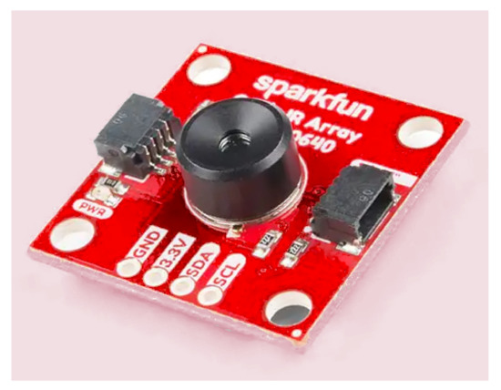
Figure 1.
The IR array sensor used for our experiments.

Table 1.
Specifications of the IR array sensor used for our experiments.
For the sake of our work, the sensor is attached to a Raspberry Pi 3 model B+. The Raspberry Pi is also equipped with a regular camera that captures the same scene as the sensor. This would allow us later to annotate the sensor data by referring to the camera images. Data on both the camera and the sensor are captured at a rate equal to eight frames per second (fps). The built system is shown in Figure 2. We use power bank to provide power to the equipment and attach the system all together and place it on the ceiling.

Figure 2.
An image of the system built to collect the sensor frames and the camera images.
4.2. Environment
As stated above, the whole system is put together and placed on the ceiling at a height h equal to m. In Figure 3, we illustrate the layout of the room and the equations according to which we extract the various measurements related to the practical coverage.
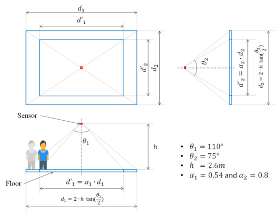
Figure 3.
The dimensions of the area covered by the sensor.
As previously mentioned and as shown in Table 1, the sensor is equipped with a wide angle lens covering, in one axis, and, in the other, . At floor level, this gives a rectangular coverage with the length and width of and , respectively, which are defined as:
However, realistically, the coverage at ground level is impractical and might lead to some detection error. As a matter of fact, if a person is standing at the edge of the coverage rectangle, only the lower part of their body (i.e., their feet) is within reach and is barely detected, as shown in the bottom left part of Figure 3. With that in mind, two coefficients and are used to ensure a reliable coverage. In view of our early studies, the values of and are set to be 0.80. This allows to cover an area of 6.0 and 3.2 m in length and width, respectively. A simplified scheme of the scenario we run as well as its corresponding frame generated is given in Figure 4.
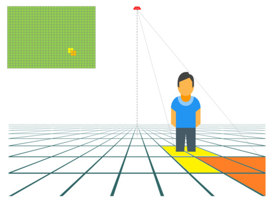
Figure 4.
A simplified example of a sensor placed on the ceiling, the coverage of its pixels and the generated frame (upper left part).
We run our experiment in 4 different rooms with different characteristics:
- Room 1: This room has a tatami covering the floor, has a large window in one of the walls and is not air conditioned. The temperature is the ambient room temperature.
- Room 2: This room also has a tatami, has a large window in one of the walls and is air conditioned (the temperature of the air conditioner is set to 24C).
- Room 3: This has a slightly reflective ground. It has no windows on the wall and is air conditioned (the air conditioner is set to heat the room to a temperature equal to 26C). The room has a desk, 4 chairs and a bed.
- Room 4: This has a slightly reflective ground. It has no windows on the wall. Instead of an air conditioner, it is heated by a heating device (stove) and a moving device (cleaning robots) were included for more variety in terms of environment conditions.
To create more variety in data, unlike our previous work [49], a new set of experiments was conducted in room 3 under a different temperature and with the inclusion of furniture. Nonetheless, a new set of experiment is run in room 4, which include furniture as well and the 2 aforementioned devices.
Multiple people from both genders (males and females) and with different body characteristics (heights and body mass) and different types of clothes participated in the experiments. Every experiment lasts for 5 min (generating almost 2400 frames), in which a group of 3 people simulate scenarios of a living room where anyone can enter or leave anytime, move in the room as they want and perform any sort of activity they want (e.g., sit, stand, walk or lay down, etc.). Data collected in every experiment are used exclusively for training or testing. In other words, all the frames collected from a single experiment are used either for training only or for testing only. This is important to avoid information leakage.
In addition, data collected to train the super resolution model have no particular constraints. All that matters is that the number of frames is high enough to let the neural network learn how to reconstruct the full-resolution image from a low-resolution one. Therefore, all frames captured for this purpose were used.
4.3. Overall System Description
In Figure 5, we show the overall flowchart of our proposed framework to be used in real scenarios: Super resolution and classification models are trained offline prior to the installation of the device. Data are collected from the sensor at a rate equal to 8 fps. Frames other than the one collected at the highest resolution (i.e., 32 × 24) are upscaled by the super resolution model. Denoising and enhancement techniques are then applied to the frames. Afterward, a classification task is run on the resulting frame to identify the number of people. Finally, we located the number of people reported by the classifier. Optionally, it would be interesting to report the activities performed by these people, in particular, in the case where a single person (i.e., the elderly person) is present in the room. This last step is dealt with in a separate work [59]. The details of the different steps are given in the next section.

Figure 5.
A flowchart of the proposed system.
5. Detailed System Description
5.1. Data Collection
As stated previously, two sets of data are collected prior to the installation of the system:
- 1.
- Super resolution data: These are data used to train and validate the super resolution model. From several experiments, we collected over 35,000 frames. We used 25,000 frames for training, 10,000 for validation and discarded a few tens of frames.
- 2.
- Classification data: These data are used to train and validate the classifier. We used different scenarios in different room environments as described in the previous section. For each resolution of frames, we used a data set composed of 25,318 frames for training and 7212 frames for testing.
In Section 6, we describe in more detail the structure of the data sets used.
5.2. Super Resolution and Frame Upscaling
This step consists of two parts: offline training and online inference. The latter part consists of simply applying the model generated offline to upscale the images collected from the sensor after its deployment. Therefore, we focus here on how the model is built and on the architecture of the neural network used.
Figure 6 shows the architecture used in the current work to perform the super resolution. This architecture follows the typical architecture of the fast super resolution convolutional neural network (FSRCNN) proposed in [60]. The neural network is composed of four major parts:
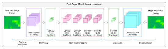
Figure 6.
The architecture of the neural network used to generate high-resolution images.
- Feature extraction and dimensionality reduction;
- Non-linear mapping;
- Expansion;
- Deconvolution.
5.2.1. Feature Extraction and Dimensionality Reduction
Here, overlapping patches of the low-resolution image are extracted and represented as a high-dimensional feature vector. They are then condensed by shrinking them to reduce the feature dimension, thus reducing noticeably the complexity and the computational cost. The first operation is conducted via an convolutional filter of size 5 × 5, while the second is conducted by using convolutional filters of size 1 × 1. While it is possible to use higher size filters, this would make training time grow drastically; therefore, these sizes are chosen.
5.2.2. Non-Linear Mapping
This operation is the core part of the super resolution architecture. The aim of this operation is to map each feature vector to another higher dimension vector showing how the “expected” output vector represents the high-resolution image. Nevertheless, the depth of this sub-network and size of filters on each of its layers have the highest impact on the performance of the super resolution performance [60]. While it is preferable to have higher filter size, such choice would impact very noticeably the speed of learning. In the current work, we adopted similar filter size to the one used in [60], i.e., 3 × 3. The number of filters per layer is referred to as and the total number of layers is referred to as m.
5.2.3. Expansion
This operation consists of expanding the high-resolution features dimension. To conduct this, a high number of filters ( filters in total) should be introduced. Therefore, this operation relies on a layer of filters of size 1 × 1 which precedes the deconvolution layer.
5.2.4. Deconvolution
This operation consists of the upsampling and aggregation of the output of the previous layer, by the means of a deconvolution layer. Deconvolution is not a commonly used function in neural networks. This is because, unlike convolution which condenses the information into a smaller one, deconvolution expands the information into a higher dimension. More accurately, this depends on the size of the stride, as a stride of size 1 with padding would give information of the same size; however, for a stride of size k, the condensed information will have a size . Inversely, a deconvolution with a stride enlarges the input information, and with an accurate choice, the output image can be the size we want.
5.2.5. Activations and Parameters
Unlike the commonly used Rectified Linear Unit (ReLU) activation function, reference [60] proposed to use Parametric ReLU (PReLU) for better learning. PReLU differs from conventional ReLU in the way that the threshold for the activation is decided. While ReLU uses 0 as a threshold, meaning that all negative values are mapped to zero, PReLU has this threshold as a parameter learned through training. This is important not only to have better training but also later on to estimate the complexity of the architecture.
In our current work, we used the following parameters for the number of filters per layer and number of non-linear mapping layers:
That being the case, the overall architecture of the super resolution network is given in Table 2.
Table 2.
The architecture of the neural network used for super resolution.
To estimate the complexity of our neural network, we use its total number of parameters as an indicator. We have a set of convolutions, a single deconvolution. To that we add the number of PReLU parameters. To recall, every convolutional layer is followed by PReLU layers.
The total number of parameters P of a given convolutional layer c is given by:
where m and n are the width and height of each filter ( in our case), p is the number of channels and k is the number of filters in the layer.
The total number of parameters P of a given PReLU layer a is given by:
where h and w are the height and width of the input image, respectively, and k is again the number of filters.
That being the case, the overall number of parameters in the network is 21,745 for the case where the input images are 8 × 6 and 47,089 for the case where the input images are 16 × 12.
5.3. Denoising and Enhancement
Before proceeding with counting the number of people, we opt for another step to further enhance the quality of the generated frames. Denoising is a well-established and explored topic in the field of computer vision and imaging in general. For the sake of simplicity, and keeping in mind the hardware limitations, in this work, we opted for three techniques to denoise the frames generated by the IR sensor.
5.3.1. Averaging over N Consecutive Frames
This method is quite straightforward: Given that the sensor collects the data at a relatively high frame rate (8 FPS), we assume that consecutive frames have little to no change with regard to the main objects/people present, unless they move at a high speed. The noise, on the other hand, changes from a frame to the next. To reduce its effect, given N consecutive frames (in practice, we use ), we average the values of pixels of two consecutive frames into one.
5.3.2. Aggressive Denoising
This method is referred to as aggressive as it suppresses a noticeable amount of information from the frame. It works on a simple principle: Frames are considered as heat matrices (raw data before transforming them into images). Adjacent pixels which are close to one another in temperature are all adjusted to their average temperature’s 0.5 upper bound. This results in a much less noisy frame, even though part of the information is lost as previously stated.
5.3.3. Non-Local Means Denoising (NLMD)
The NLMD [61] method is based on a straightforward principle and works on images as images rather than heat matrix: replacing a pixel’s color with an average of the colors of similar pixels. However, the pixels that are most similar to a particular pixel have no need to be near close to it at all. Thus, it is permissible to scan a large section of the picture in search of all pixels that closely match the pixel to be denoised. Obviously, this technique is more expensive in terms of computation, yet it is still considered as cost effective.
In Figure 7, we show (a) examples of frames captured for when there is (are) one participant, two participants or three participants, (b) examples of frames denoised using the aggressive method and (c) frames denoised using NLMD. As can be observed, after applying the two denoising techniques, the amount of noise is reduced remarkably. Later, in the experimental results section, we discuss the importance of this step, as well as whether it is relevant and worth the extra computation cost or not.

Figure 7.
Examples of frames denoised using different techniques. (a) Original Frames, (b) Frames “aggressively” denoised, (c) Frames denoised using NLMD.
While other more effective techniques exist in the literature that address the task of noise reduction/removal [62,63,64], such techniques come at a cost in terms of computation power and time. This cost defies our objective of making the approach run on low-end devices in real time. In a future work, we will address the task of noise reduction in low-resolution thermal images and perform a more thorough analysis of the different techniques to identify which presents the best performance to cost ratio.
5.4. Counting People
Upon upscaling, the output images go through the classification neural network. The network will take as input the super resolution version of the frame captured by the sensor. The classification will have as output the number of people detected.
For the classification, similar to our work [59], we opted for a lightweight neural network for the classification in both cases. In the current work, we trained the neural network from scratch to perform the classification. In [59], we made use of the network trained here and applied transfer learning for classification. This is because the data available for the task of counting people are much more abundant. As shown in Figure 5, both models are made to work together in the same device using their respective models.
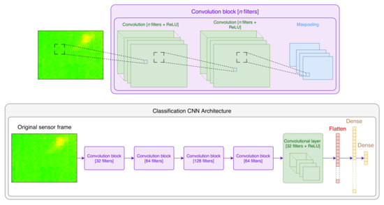
Figure 8.
The architecture of the neural network used for classification.
Table 3.
The architecture of the neural network used for classification.
The upper part of Figure 8 shows the structure of a convolutional block: such a block has two convolutional layers with a ReLU activation, followed by a Max pooling layer. Each convolutional layer consists of a set of n filters of size , whose weights are initialized randomly and learned over training. In addition, we added padding to the edges of the frames to prevent the sizes of the generated images (except when performing Max pooling) from decreasing.
The lower part of Figure 8 shows the overall architecture of our proposed model: it consists of four convolution blocks followed by a flattening layer and two dense layers. The last dense layer is obviously one responsible for determining the class. Therefore, all layers have ReLU activations except for the last dense layer whose activation is a Softmax. Moreover, we used a drop out equal to 0.6 after each Max pooling layer.
Again, the number of parameters is used as a measure of the complexity of the network. In addition to Equations (4) and (5), we use the following equation to calculate the total number of parameters P of a given dense layer d:
where s is the size of the dense layer (the number of neurons) and t is the number of neurons in the previous layer.
The total number of parameters of the classification neural network is about 410 K parameters. To put that into perspective, a network architecture such as ResNet34 [20] has a total number of parameters that is about 21 M and VGG16 [21] has a total number of parameters that is about 138 M. In case we want to run everything locally on a device such as the Raspberry Pi, equipped with a Movedius Neural Stick (https://software.intel.com/en-us/movidius-ncs. Accessed 7 November 2021), simpler architectures such as ours would not consume much computational resources and would run in real time with a frame rate equal to eight.
As stated above, it is important to keep in mind that our objective is to run the models on a low-end device. Therefore, having light neural network architecture is one of the constraints we have set when designing it. With that in mind, the number of layers and filters per layer have been set to the smallest number possible. Nonetheless, given that the characteristics of hardware (in general) work more efficiently when memory chunks stored in powers of two are passed, the batch size and other parameters were set to be as such. This is a common practice in the community and explained in reference [65]. We have tried using different network architectures with more (respectively, less) layers. In the former case (i.e., using deeper networks), there is no noticeable gain in the classification performance that justifies the extra computation cost. In the latter case, using shallower networks does indeed affect the performance: the classification accuracy drops significantly and cases when a person is laying on the ground or people are very close to each other would result in misclassification.
To summarize, despite being simplistic, the proposed architecture provides very good classification results. In addition, due to its simplicity, once trained, it can run the classification fast enough even on a low computational device such as the Raspberry Pi itself. The classification objective is to count the number of people. In our experiments, at a given time, the room could have zero, one, two or three people. Therefore, four classes are present in total.
5.5. Identification of the Location of People
This step uses the same method we previously used in [49]. The previous step outputs the number of people present in the room, which we refer to as N. After identifying N, we use a method referred to, in the computer vision world, as Canny’s edge detection [66]. Canny’s edge detection approach is widely employed in computer vision to identify edges of objects in images. The approach relies on the difference in color between the adjacent pixels. The detailed description of the approach is given in [66]. In our work, using [66], we aim to find the top N hottest spots in the sensor image. We briefly summarize the steps taken by this method to detect edges in an image:
- 1.
- Noise Reduction: To facilitate the detection, the first step, as its name implies, is to reduce the image noise. The way this is performed is by using a Gaussian filter to smoothen the frame.
- 2.
- Find the intensity gradient: After reducing the noise, the intensity gradient of colors in the image are derived. To achieve this goal, a Sobel kernel filter [67] is applied on the horizontal and vertical directions. This would allow us to obtain the corresponding respective derivatives and , which, in return, are used to obtain the gradient and orientation of pixels:
- 3.
- Suppression of non-maximums: Edges are, by definition, local maximums. Hence, non-local maximum pixels (obviously in the direction of the gradients measured in the previous step) are discarded. Nevertheless, during this step, fake maximums (i.e., pixels whose gradient is equal to 0, but they are not actual maximums) are identified and discarded.
- 4.
- Double thresholds and hysteresis thresholding: While in the previous step, non-edge pixels are set to 0, edges have different intensities. This step suppresses—if necessary—weak edges (i.e., edges that do not separate two objects or an object from its background). Obviously, the definition of a weak edge implies a subjective decision. This is achieved thanks to two parameters that need to be taken into account: an upper threshold and a lower one.
One thing to retain is that these last two parameters (thresholds) can drastically change the level of details captured and by how much the values of the neighboring pixels should differ for an edge to be detected. The approach can be made more or less sensitive to “color” nuances by tweaking these thresholds. Consequently, detected edges can reflect sharper or smaller changes in temperature.
Given the nature of our images (i.e., pixel frames reflecting heat emitted by objects in the room), we set default values for these thresholds so that they detect the N hottest spots correctly, most of the time. This implies that in some cases they do not work correctly. Therefore, these values are dynamically adjusted if the number of hot spots detected is different from N (it is increased if the detected number is different from N and vice versa). We then identify the centroids of areas found and consider them to be the approximate locations of the people present in the room.
5.6. Activity Detection
In a separate work of ours [59], we used the same equipment to run another classification task whose goal is to detect the activity performed by a person present in the room. While this is out of the scope of the current paper, it might be worth mentioning that the accuracy of activity detection reported for seven different types of activities reached over 97%.
6. Experimental Results
6.1. Data Sets
To evaluate the performance (i.e., accuracy of detection, precision and recall) of the approach that relies on super resolution for identifying and counting people, we use a data set identical in size for all resolutions that we experimented with: 8 × 6-size, 16 × 12-size and 32 × 24-size frames. The structure of the data set is given in Table 4.
Table 4.
Data sets used: the number of frames with N people present in them, .
6.2. High-Resolution Classification Results
6.2.1. Training Set Cross-Validation
To measure the correctness of classification, we use four Key Performance Indicators (KPIs), which are the TP rate, precision, recall and the F1-score. In a first step, we perform a 5-fold cross-validation on the training set. The training set is split into five subsets. In each fold, three of the subsets are used to train a model, one is used for validation and one is used for evaluation.
Since different techniques of denoising have been used in our work, we first report the overall classification KPIs averaged over all the folds using each technique, as well as that for the original frames. We use the following terminology for the following methods of denoising of the frames:
- The method where frames captured with size 32 × 24 with no denoising is referred to as ();
- The method where frames captured with size 32 × 24 are denoised by averaging over two consecutive frames is referred to as ();
- The method where frames captured with size 32 × 24 are denoised by the aggressive denoising method is referred to as ();
- The method where frames captured with size 32 × 24 denoised by the NLMD method [61] is referred to as ().
In Table 5, we show the overall the reported performance.
Table 5.
The classification TP rate, precision, recall and F1-score of the high-resolution frames during cross-validation for different denoising techniques.
Since the use of NLMD [61] has given the highest KPIs, we focus on this technique and report in Table 6 the classification results on each of the individual folds, as well as the weighted average of them for the method ().
Table 6.
The classification TP rate, precision, recall and F1-score of the high-resolution frames during cross-validation.
6.2.2. Evaluation on the Test Set
Here, we use the entire training to train and validate one more model and use the trained model on unseen data. After training our model, we run the classification on our test set. The results of classification are given in Table 7, and the confusion matrix of classification is given in Table 8. Similar to cross-validation, the evaluation here is performed using the best-performing denoising technique (i.e., the NLMD method [61]).
Table 7.
The classification TP rate, precision, recall and F1-score of the high-resolution frames on the test set.
Table 8.
The classification confusion matrix of the high-resolution frames on the test set.
The overall accuracy obtained reaches over 97.67%, with a precision and recall of the class 0 (class 0 represents the case where no person is present in the room) equal to 100%. This means that it is possible to confirm, at any given moment, whether or not there is someone in the room. This is of utmost importance, given that one of our goals, at the end of the day, is to monitor the person when they are in the room. Being able to identify their presence when true should be certain with 100% confidence.
Location-wise, it is hard to confirm the level of precision of detection due to the fact that different pixels of the generated sensor image cover different area sizes due to the angle difference. In addition, due to the distortion in the image captured by the camera, the exact location cannot be confirmed at a very precise level. Nevertheless, we rely on the centroids of the generated areas to determine the location of users. This makes the exact location not very accurate. Our empirical measurements show that the margin of inaccuracy is about 0.3 m. With that in mind, it is fair to affirm that the location identification reaches 100% accuracy for the correctly classified instances and for the precision level mentioned (i.e., 0.3 m). In other words, for the frames where we were able to correctly identify the number of people present, the objects detected as the participants, using the Canny’s method for edge detection, correspond indeed to them. In Figure 9, we show an example of some instances correctly classified and whose location are correctly identified.
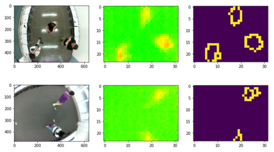
Figure 9.
Examples of the same instant as captured by the camera (left), the sensor (middle) and processed sensor frames to identify the location of detected people (right).
6.3. Low-Resolution Classification Results
6.3.1. Super Resolution: How to Evaluate the Performance
In Figure 10, we show an example of two consecutive frames collected with size 32 × 24. The frames show the existance of three people in the room. As we can observe, in the regions of low temperatures, the amount of noise present is very high, leading to a grid effect: nearby pixels have a trend to oscillate so that each pixel has values that are higher/lower than the neighboring ones and pixels change from being higher to being lower than its neighbors in consecutive frames.
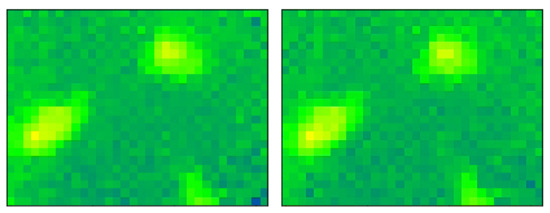
Figure 10.
An example of two consecutive frames to show the amount of noise present in them. The total number of people present in the room is 3. However, other than the hotspots which correspond to these people, the other pixels’ values (colors) fluctuate remarkably.
Given that the amount of such noise in the frames captured by the sensor is high, we did not evaluate the performance of the super resolution approach using the conventional metrics of evaluation of super resolution (e.g., entropy). We relied, instead, on the actual classification that takes place when we count people. In other words, if the classification accuracy is improved compared to the original low-resolution images, we conclude that the super resolution approach is good and has contributed to enhancing the performance of our classifier.
In addition, to observe the effect of minimizing the noise, we have added an evaluation of frames generated using the different techniques described previously in Section 5.3. In total, we evaluate the classification performance of the following methods of capturing the frames:
- The method where frames captured with size 32 × 24 are used as they are is referred to as ();
- The method where frames captured with size 32 × 24 are denoised by the NLMD method [61] is referred to as ();
- The method where frames captured with size 16 × 12 are used as they are is referred to as ();
- The method where frames captured with size 16 × 12 are upscaled with the super resolution technique to 32 × 24 is referred to as ();
- The method where frames captured with size 16 × 12 are upscaled with the super resolution technique to 32 × 24 and denoised by averaging over two consecutive frames is referred to as ();
- The method where frames captured with size 16 × 12 are upscaled with the super resolution technique to 32 × 24 and denoised by the aggressive denoising method is referred to as ();
- The method where frames captured with size 16 × 12 are upscaled with the super resolution technique to 32 × 24 and denoised by the NLMD method [61] is referred to as ();
- The method where frames captured with size 8 × 6 are used as they are is referred to as ();
- The method where frames captured with size 8 × 6 are upscaled with the super resolution technique to 32 × 24 is referred to as ();
- The method where frames captured with size 8 × 6 are upscaled with the super resolution technique to 32 × 24 and denoised by averaging over two consecutive frames is referred to as ();
- The method where frames captured with size 8 × 6 are upscaled with the super resolution technique to 32 × 24 and denoised by the aggressive denoising method is referred to as ();
- The method where frames captured with size 8 × 6 are upscaled with the super resolution technique to 32 × 24 and denoised by the NLMD method [61] is referred to as ().
6.3.2. Classification Results
Training set cross-validation: To evaluate the different methods introduced above by performing 5-fold cross-validation, we use the same seeds for their respective data. The results of cross validation are given in Table 9. For simplicity, we report only the performance averaged over the 5 folds for each method.
Table 9.
The classification TP rate, precision, recall and F1-score during cross-validation.
As we can observe from the results, the introduction of super resolution remarkably improves the performance of the classification for both frames of size 8 × 6 and 16 × 12. Enhancing the frames by averaging over two consecutive ones further improves the performance as shown in Table 9.
Evaluation on the test set: The results of classification using the different methods are given in Table 10. In addition, for the particular methods where super resolution is used with enhancement by averaging over two consecutive frames ( and ), the confusion matrices are given in Table 11 and Table 12, respectively.
Table 10.
The classification TP rate, precision, recall and F1-score on the test set.
Table 11.
The classification confusion matrix of the method on the test set.
Table 12.
The classification confusion matrix of the method on the test set.
As we can observe from Table 10, when using the low-resolution frames ( and ), we obtained much lower classification performance than when using the full resolution ().
However, we can also observe that, after applying the super resolution techniques and enhancing the frames by averaging over two consecutive ones, the accuracy of classification is highly increased. The accuracy using upscaled and enhanced 8 × 6 frames (method ) reaches 86.79% and that using upscaled and denoised 16 × 12 frames (method ) reaches 94.90%.
This is by no means close to the results of classification of frames originally of size 32 × 24, in particular, for the method . However, such results present a good starting point for our next work where we intend to use a Long Short-Term Memory (LSTM) in addition to the CNN to evaluate based on few consecutive frames. We believe that the use of an LSTM will help overcome the misclassification of few frames by learning over a longer period of time how to make more accurate judgements. In addition, the recall and precision of the class 0 (which aims to identify whether or not there is a person in the room) reach 97.00 and 97.90%, respectively, for the method . These metrics reach 99.46 and 99.69%, respectively, for the method .
Location-wise, as mentioned earlier, we used the same method described in [49]. This method has proven to be very good as it detected the N largest hot areas in a frame, where N is the number of people returned by the classifier.
We do not describe the details of the method, as it is given in our previous work [49].
6.4. Discussion
In the previous sub-sections, we have shown how it is possible to provide good classification accuracy when employing super resolution techniques. The results returned by the classification of upscaled and denoised frames are comparable to those of high-resolution ones. In particular, when using the original sensor frames of size , the detection accuracy difference is less than 2%. That being said, despite reaching good performance, the current method has lower classification performance than that of higher resolution frame. We believe that it is possible to remedy this problem by using an LSTM neural network built on top of the CNN (i.e., uses the output of the CNN). Here, we suggest to use several consecutive frames. By observing over multiple frames the people present, it would be possible to detect more accurately their number and identify more accurately their location. In other words, even if individual frames can have wrong detections here and there, when using consecutive frames, such error could be minimized.
On a more interesting side, our experiments have shown that it is possible to identify multiple people present with good accuracy, even when these people are close to one another. For instance, in Figure 11, we show an example of a frame that has been misclassified when using the method and correctly classified upon applying super resolution. The low-resolution frame does not include enough information for the classification model to identify the presence of two people. Upon upscaling with super resolution techniques, the two people present were easily identifiable by the classifier.
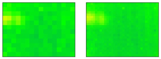
Figure 11.
An example of a frame misclassified on its original size and correctly classified upon upscaling. The low-resolution frame (left) has been classified as if there is one person in the room. Upon upscaling the frame (right), the classifier managed to identify two different people in the frame.
It is important here to emphasize the fact that super resolution, unlike conventional image enhancement techniques, learns more latent features and details specific to the nature of images themselves (heat-maps, in our case). These features and details help, in their turn, to rebuild a higher resolution frame, faithful to the actual heat distribution, something that cannot be performed otherwise. As a matter of fact, using the bicubic algorithm [68] to upscale the small frames has led to a decrease in detection accuracy, even compared to the original low-resolution frames. Through learning, the super resolution neural network manages to learn how to appropriately identify the edges and the color intensity of the objects, leading to a much more accurate classification by the classifier.
That being said, the current approach has a few limitations that are worth mentioning and which we will address in a future work:
- 1.
- The actual misclassification: As it stands, the current model does not give perfect detection accuracy, even when using the high-resolution frames (i.e., 32 × 24 pixels). As stated above, we believe that the use of LSTM would remedy the problem of misclassification of individual frames by learning over longer periods of time the number and locations of people.
- 2.
- The presence of heat-emitting devices/objects: Devices emitting heat include electronic devices such as computers, heaters or even large open windows allowing for the sunlight to enter the room. Such devices or objects could lead to a misclassification as their heat might be confused with that emitted by a human body. This problem can be also addressed by exploiting the time component. Unlike the first issue we mentioned about the use of few consecutive frames, learning here requires the observation over much longer periods of time that can go to hours to learn the overall behavior of the non-human heat emitters in the room.
- 3.
- The residual heat in furniture (e.g., a bed or a sofa) after a person spends a long time on it: After leaving their bed/seat, the heat absorbed by the piece of furniture will be emitted, leading to a wrong identification of the person. This heat, despite dissipating after a while, is not to be confused by the heat emitted by the person themself. This could be addressed by learning this particular behavior and taking it into account when making the classification decision.
- 4.
- The presence of obstacles: The presence of obstacles is an inherent problem with object detection systems that rely on direct line of sight between the sensor and the object to be detected. This problem can partially be addressed by design choices as for where to place the sensor or by using multiple sensors that cover the entire area of monitoring.
In a future work, we will be mainly focusing on the three first limitations. We will make use of short- and long-term residual information to identify which constitutes a real representation of a human and which does not. We will also address the problem of the detection of actions of each person individually by isolating their representation using object identification techniques and applying the activity detection technique we propose in [59] to identify their activity.
7. Proposed Approach against State-of-the-Art Object Detection
In this section, we describe in more detail the idea behind RetinaNet [52] and what makes it much more powerful than other object detection neural network architectures. We then compare the results of our proposed method to RetinaNet [52] in terms of classification and detection accuracy but, more importantly, in execution time, as our proposed method aims to run the detection on low-end devices with very limited computational power.
Besides RetinaNet, we compare our approach against a Dense Neural Network (DNN), composed of:
- A flattening layer to transform the input image into a uni-dimensional vector.
- A total of 4 fully-connected dense layers having, respectively, 512, 256, 128, 64 neurons, whose activation is set to ReLU.
- A fully-connected layer with a Softmax activation responsible for determining the class.
The same technique we proposed for localization is used here after the classification.
7.1. RetinaNet
The RetinaNet [52] model architecture is shown in Figure 12. The architecture is composed of three main components:
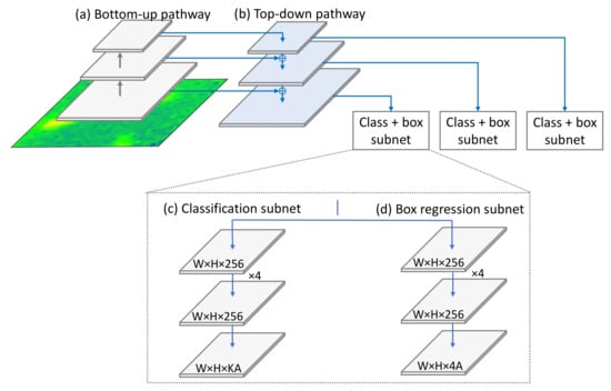
Figure 12.
RetinaNet’s simplified architecture. This network is composed of four parts: (a) bottom-up pathway, (b) top-down pathway, (c) classification subnet and (d) anchor regression subnet.
- 1.
- The backbone: The backbone calculates the feature maps at different scales. This is usually a typical convolutional network that is responsible for computing the feature map over the input image. In our work, we opted for the conventional ResNet34 architecture [20] as a backbone for RetinaNet. It has two parts:
- The bottom-up pathway: here, the backbone network calculates the feature maps at different scales.
- The top-down pathway: the top-down pathway upsamples the spatially coarse feature map. Lateral connections merge the top-down layers and bottom-up layers whose size are the same.
- 2.
- The classification subnet: This subnet predicts the probability of an object of a given class being present in each anchor box.
- 3.
- Anchor regression subnet: Upon identifying objects, this network offsets the bounding boxes from the anchor boxes for the objects.
Despite its performance, the idea behind RetinaNet is quite simple: Using the concept of anchor boxes, RetinaNet creates plural “sub-images” that cover various areas within the image. Afterward, a classification task is performed to identify classes of the smaller images. If an object is identified with a certain confidence, the network proceeds to finding the accurate bounding box of the object. The backbone has for objective the generation of feature map. The two sub-networks perform convolutional object classification and bounding box regression.
We used the Fastai [69] implementation of RetinaNet available on GitHub (https://github.com/ChristianMarzahl/ObjectDetection Accessed 29 January 2022). Fastai allows for an easier tweak of parameters to make the detection run faster if needed. This will be explained in more detail in the rest of this section. The implementation requires the data ground truth to be formatted in the MS. COCO [70] format. Obviously, we have a single class here, which we called “person”. We used the LabelBox (https://labelbox.com/ Accessed 29 January 2022) services to annotate the data. Given the requirements of RetinaNet, all images have been upscaled to 320 × 240, which we labeled using LabelBox. We use RetinaNet34 [20] as a backbone architecture.
Given that the images are upscaled and each pixel is replaced by a 10 × 10 pixels, we have discarded multiple possible anchor boxes. This is because the bounding boxes of objects have x and y coordinates (and widths and heights as well) that need to be multiples of 10. Performing such will reduce the computational tasks.
7.2. Results Comparison
To measure the accuracy of detection (counting people), we do not use the common object detection metrics such as Average Precision (AP) and mean Average Precision (mAP). We opted for a more straightforward metric that allows for a fair comparison with our proposed method. For each image classified by RetinaNet, we count the number of detected objects and compare it to the ground truth.
In terms of computation speed, we run the object detection task on the entire test set and average it by dividing it by the total number of frames in the test set. A final comparison will be performed (though not as important) which consists of comparing the classification of the ground truth images collected by the camera to the classification of the heat frames collected by the sensor. This will be conducted to show the potential of RetinaNet in real-world images as opposed to heat frames.
Being part of our proposal, we did not apply the super resolution technique on the lower resolution images (i.e., ) before using RetinaNet. In other words, frames of size 8 × 6 are upscaled to 640 × 480 without applying the super resolution technique first. Nevertheless, bicubic interpolation has not been applied as the images become very blurry and RetinaNet is penalized when such method is applied.
In Table 13, we show the results of detection using our proposed approach using the methods (), () and () against RetinaNet applied on the lowest resolution frames (i.e., ) and the highest resolution ones (i.e., 32 × 24). As can be seen, our method provides lower performance for the highest resolution frames. Obviously, the high complexity of RetinaNet and its deep network backbone (ResNet) have the upper edge over our low complexity network. However, the results show that the difference between the two methods is not large, and given the difference in complexity, we do believe that our method has its merits and provides good results.
Table 13.
The classification TP rate, precision, recall, and F1-score of the proposed method vs. the conventional ones.
More interestingly, when applied on the lowest resolution images, our method performs better than RetinaNet. As stated above, the super resolution is used exclusively as part of our method, and therefore, upscaled raw data are used as input for RetinaNet. This has given our method a better reconstruction of the original images, allowing for a better detection of people.
In Table 14, we compare the results of detection of people using RetinaNet applied on the camera-collected images and the IR sensor-collected ones. As we can observe, RetinaNet almost reaches perfect results when processing real images. This is because camera images are much richer in terms of features, and RetinaNet’s deep backbone network (ResNet34) is very powerful processing large size images.
Table 14.
The classification TP rate, precision, recall, and F1-score of RetinaNet on camera images (cam) vs. heat frames (HF).
For a final comparison, we run the two approaches and compare the processing of images. While training time varies drastically between the models (few minutes for our method, against several hours for RetinaNet), we do believe that the implementation contributes to this difference and therefore compare the detection using trained models on the test set. Since we were unable to run RetinaNet on the Raspberry Pi, we compare the results when running the approaches on a regular Desktop equipped with an Nvidia GPU of type GTX1080Ti. The results are given in Table 15. It is obvious that our method is much faster than RetinaNet. This allows our approach to be implemented to perform the detection in real time.
Table 15.
Execution time of the proposed approach and the conventional ones.
Overall, our method, despite its simplicity, reaches performance comparable to that of cutting-edge object identification techniques. Obviously, it is applicable only to IR sensor frames, as these are quite simplistic and do not contain much information, which makes the edge detection technique more than enough to identify existing heat-emitting objects in the scene. Nonetheless, thanks to its simplicity, our method is much faster than RetinaNet and could be used to run real-time detection even for 16 FPS-collected data.
It is worth mentioning that, given that the objective of RetinaNat is not the classification but rather the detection, a few frames were reported by RetinaNet as containing four people, as if the model has detected four distinct objects. This could be seen as a limitation but also an advantage of RetinaNet compared to our proposed approach: On the one hand, in our method, the classification precedes the detection, and the number of people is defined before looking for them. On the other hand, RetinaNet does not require re-training to identify more people in the scene even if it has been trained with at most three people per frame, whereas our method cannot detect more than three people, and in order to be able to detect more, the entire model needs to be retrained again with more data.
Another point worth noting is that our method does not require manual annotation of objects’ locations. RetinaNet, on the opposite side, requires manual annotation of the data. For each training instance, our method requires only annotating the image by giving it the number of people present, which could be easily achieved by referring to the camera image. RetinaNet, on the other hand, requires the annotator to specify the coordinates of each object (i.e., x and y coordinates of the top-left vertex of the bounding box of the object and its width and height), which is tedious work that requires time and effort.
7.3. Discussion
Throughout this work, we have demonstrated that it is possible to use low-end sensors running on computation capability-limited devices to perform device-free indoor counting and localization. That being said, in the literature, many other works have been proposed to perform such a task. These come with their respective advantages and shortcomings and have varying detection performance. In this subsection, we put into perspective our proposal against some of these works. In Table 16, we summarize the main results reported by these works and highlight their main advantages, shortcomings and reported results.
Table 16.
Comparison with existing methods for indoor localization.
As can be observed, a main drawback common to these methods is their reliance on portable devices to perform the detection. Nonetheless, [38,40] require expensive equipment to run. A device-free solution is a challenging task and is practically unfeasible using technologies that rely on ambient signals, such as WiFi and Bluetooth ones. Promising attempts [45,46,47] have been proposed in the literature to perform a quite related task (i.e., fall detection) by observing the change in the environment signals. However, extending such an idea for localization or counting is much more challenging.
Device-free detection requires “meaningful” information to be detected from the body of people present. This could be achieved using cameras or 3D LiDARs, for example, which would perform near-perfect detection, though pose privacy issues. IR array sensors, which are proposed to be used in this work, detect the heat emitted by the body and maps it into a very low-resolution image. This allows for a good detection while preserving the privacy of people. Our experiments showed that this approach is indeed capable of reaching high performance.
8. Conclusions
In this paper, we proposed an extension to a previous approach to detect the presence/absence of people in a room and count the number of people present using a low-resolution sensor. Similar to our previous work [49], we initially used the sensors with their highest resolution (i.e., 32 × 24 pixels). Our approach achieved good performance in the identification of the presence of up to three people with an accuracy reaching 97.5%. Nevertheless, in the case of a single person’s presence/absence, the accuracy reaches 100%. However, since lower resolution sensors come at a much cheaper price in the market, we introduced an approach to improve the quality of images generated by such sensors and applied the same technique described above to perform the classification and detection tasks. For this sake, we first applied techniques of super resolution and CNN to upscale and enhance the frames collected at a lower resolution (16 × 12 and 8 × 6) and to run classification on the captured frames. The proposed approach identifies the presence of up to three people with an accuracy reaching 94.66% and detects the presence/absence of a person with over 99% accuracy. The approach also served to identify the location of people with a margin of 0.3 m. This allowed us to build an autonomous device (based on a Raspberry Pi 3 model B+) capable of counting and locating people using the trained models.
Author Contributions
Conceptualization, M.B. and C.Y.; methodology, M.B.; software, M.B. and C.Y.; validation, M.B. and C.Y.; formal analysis, M.B.; resources, M.B.; data curation, M.B.; writing—original draft preparation, M.B., C.Y. and T.O.; writing—review and editing, M.B. and T.O.; supervision, T.O. All authors have read and agreed to the published version of the manuscript.
Funding
This research received no external funding.
Institutional Review Board Statement
Not applicable.
Informed Consent Statement
Not applicable.
Data Availability Statement
Not applicable.
Conflicts of Interest
The authors declare no conflict of interest.
Abbreviations
The following abbreviations are used in this manuscript:
| CNN | Convolutional Neural Network |
| DL | Deep Learning |
| FPS | Frames Per Second |
| FPRCNN | Fast Super Resolution Convolutional Neural Network |
| GPS | Global Positioning System |
| IR | Infrared |
| KPI | Key Performance Indicator |
| NLMD | Non-Local Means Denoising |
| PReLU | Parametric Rectified Linear Unit |
| SSD | Single Shot MultiBox Detector |
| TP | True Positives |
References
- Ketu, S.; Mishra, P.K. Internet of Healthcare Things: A contemporary survey. J. Netw. Comput. Appl. 2021, 192, 103179. [Google Scholar] [CrossRef]
- Perera, M.S.; Halgamuge, M.N.; Samarakody, R.; Mohammad, A. Internet of things in healthcare: A survey of telemedicine systems used for elderly people. In IoT in Healthcare and Ambient Assisted Living; Springer: Berlin/Heidelberg, Germany, 2021; pp. 69–88. [Google Scholar]
- Yang, S.; Wang, D.; Li, W.; Wang, C.; Yang, X.; Lo, K. Decoupling of Elderly Healthcare Demand and Expenditure in China. Healthcare 2021, 9, 1346. [Google Scholar] [CrossRef] [PubMed]
- Hamiduzzaman, M.; De Bellis, A.; Abigail, W.; Kalaitzidis, E.; Harrington, A. The world is not mine–barriers to healthcare access for Bangladeshi rural elderly women. J. Cross-Cult. Gerontol. 2021, 36, 69–89. [Google Scholar] [CrossRef] [PubMed]
- Yotsuyanagi, H.; Kurosaki, M.; Yatsuhashi, H.; Lee, I.H.; Ng, A.; Brooks-Rooney, C.; Nguyen, M.H. Characteristics and healthcare costs in the aging hepatitis B population of Japan: A nationwide real-world analysis. Dig. Dis. 2022, 40, 68–77. [Google Scholar] [CrossRef]
- Qian, K.; Zhang, Z.; Yamamoto, Y.; Schuller, B.W. Artificial intelligence internet of things for the elderly: From assisted living to health-care monitoring. IEEE Signal Process. Mag. 2021, 38, 78–88. [Google Scholar] [CrossRef]
- World Health Organization. WHO Global Report on Falls Prevention in Older Age. Available online: https://www.who.int/ageing/publications/Falls_prevention7March.pdf (accessed on 29 January 2022).
- Wang, J.; Zhai, S. Heart Rate Detection with Multi-Use Capacitive Touch Sensors. U.S. Patent 10,299,729, 28 May 2019. [Google Scholar]
- Rosales, L.; Skubic, M.; Heise, D.; Devaney, M.J.; Schaumburg, M. Heartbeat detection from a hydraulic bed sensor using a clustering approach. In Proceedings of the 2012 Annual International Conference of the IEEE Engineering in Medicine and Biology Society, San Diego, CA, USA, 28 August–1 September 2012; pp. 2383–2387. [Google Scholar]
- Luo, F.; Poslad, S.; Bodanese, E. Temporal convolutional networks for multiperson activity recognition using a 2-d lidar. IEEE Internet Things J. 2020, 7, 7432–7442. [Google Scholar] [CrossRef]
- Ma, Z.; Bigham, J.; Poslad, S.; Wu, B.; Zhang, X.; Bodanese, E. Device-free, activity during daily life, recognition using a low-cost lidar. In Proceedings of the 2018 IEEE Global Communications Conference (GLOBECOM), Abu Dhabi, UAE, 9–13 December 2018; pp. 1–6. [Google Scholar]
- Mashiyama, S.; Hong, J.; Ohtsuki, T. A fall detection system using low resolution infrared array sensor. In Proceedings of the 2014 IEEE 25th Annual International Symposium on Personal, Indoor, and Mobile Radio Communication (PIMRC), Washington DC, USA, 2–5 September 2014; pp. 2109–2113. [Google Scholar]
- Mao, G.; Fidan, B.; Anderson, B.D. Wireless sensor network localization techniques. Comput. Netw. 2007, 51, 2529–2553. [Google Scholar] [CrossRef] [Green Version]
- Sen, S.; Radunovic, B.; Choudhury, R.R.; Minka, T. You Are Facing the Mona Lisa: Spot Localization Using PHY Layer Information. In Proceedings of the 10th International Conference on Mobile Systems, Applications, and Services, Lake District, UK, 25–29 June 2012; Association for Computing Machinery: New York, NY, USA, 2012; pp. 183–196. [Google Scholar]
- Lim, H.; Kung, L.C.; Hou, J.C.; Luo, H. Zero-Configuration, Robust Indoor Localization: Theory and Experimentation. In Proceedings of the IEEE INFOCOM 2006. 25TH IEEE International Conference on Computer Communications, Barcelona, Spain, 23–29 April 2006; pp. 1–12. [Google Scholar]
- Nandakumar, R.; Chintalapudi, K.K.; Padmanabhan, V.N. Centaur: Locating devices in an office environment. In Proceedings of the 18th Annual International Conference on Mobile Computing and Networking, Istanbul, Turkey, 22–26 August 2012; pp. 281–292. [Google Scholar]
- Mobark, M.; Chuprat, S.; Mantoro, T. Improving the accuracy of complex activities recognition using accelerometer-embedded mobile phone classifiers. In Proceedings of the 2017 Second International Conference on Informatics and Computing (ICIC), Jayapura, Indonesia, 1–3 November 2017; pp. 1–5. [Google Scholar]
- Atallah, L.; Lo, B.; King, R.; Yang, G.Z. Sensor placement for activity detection using wearable accelerometers. In Proceedings of the 2010 International Conference on Body Sensor Networks, Biopolis, Singapore, 7–9 June 2010; pp. 24–29. [Google Scholar]
- Zhang, D.; Xia, F.; Yang, Z.; Yao, L.; Zhao, W. Localization technologies for indoor human tracking. In Proceedings of the 2010 5th International Conference on Future Information Technology, Busan, Korea, 21–23 May 2010; pp. 1–6. [Google Scholar]
- He, K.; Zhang, X.; Ren, S.; Sun, J. Deep residual learning for image recognition. In Proceedings of the IEEE Conference on Computer Vision and Pattern Recognition, Las Vegas, NV, USA, 27–30 June 2016; pp. 770–778. [Google Scholar]
- Simonyan, K.; Zisserman, A. Very deep convolutional networks for large-scale image recognition. arXiv 2014, arXiv:1409.1556. [Google Scholar]
- Mathie, M.; Coster, A.; Lovell, N.; Celler, B. Detection of daily physical activities using a triaxial accelerometer. Med. Biol. Eng. Comput. 2003, 41, 296–301. [Google Scholar] [CrossRef]
- Bao, L.; Intille, S.S. Activity recognition from user-annotated acceleration data. In International Conference on Pervasive Computing; Springer: Berlin/Heidelberg, Germany, 2004; pp. 1–17. [Google Scholar]
- Lo, B.; Atallah, L.; Aziz, O.; El ElHew, M.; Darzi, A.; Yang, G.Z. Real-time pervasive monitoring for postoperative care. In Proceedings of the 4th International Workshop on Wearable and Implantable Body Sensor Networks (BSN 2007), Aachen, Germany, 26–28 March 2007; Springer: Berlin/Heidelberg, Germany, 2007; pp. 122–127. [Google Scholar]
- Cornacchia, M.; Ozcan, K.; Zheng, Y.; Velipasalar, S. A survey on activity detection and classification using wearable sensors. IEEE Sens. J. 2016, 17, 386–403. [Google Scholar] [CrossRef]
- Liu, T.; Guo, X.; Wang, G. Elderly-falling detection using distributed direction-sensitive pyroelectric infrared sensor arrays. Multidimens. Syst. Signal Process. 2012, 23, 451–467. [Google Scholar] [CrossRef]
- Want, R.; Hopper, A.; Falcao, V.; Gibbons, J. The active badge location system. ACM Trans. Inf. Syst. (TOIS) 1992, 10, 91–102. [Google Scholar] [CrossRef]
- LLC, M. Firefly Motion Tracking System User’s Guide. Available online: http://www.gesturecentral.com/firefly/FireflyUserGuide.pdf (accessed on 29 January 2021).
- Hou, X.; Arslan, T. Monte Carlo localization algorithm for indoor positioning using Bluetooth low energy devices. In Proceedings of the 2017 International Conference on Localization and GNSS (ICL-GNSS), Nottingham, UK, 27–29 June 2017; pp. 1–6. [Google Scholar]
- Radoi, I.E.; Cirimpei, D.; Radu, V. Localization systems repository: A platform for open-source localization systems and datasets. In Proceedings of the 2019 International Conference on Indoor Positioning and Indoor Navigation (IPIN), Pisa, Italy, 30 September–3 October 2019; pp. 1–8. [Google Scholar]
- Dinh-Van, N.; Nashashibi, F.; Thanh-Huong, N.; Castelli, E. Indoor Intelligent Vehicle localization using WiFi received signal strength indicator. In Proceedings of the 2017 IEEE MTT-S International Conference on Microwaves for Intelligent Mobility (ICMIM), Aichi, Japan, 19–21 March 2017; pp. 33–36. [Google Scholar]
- Zhu, J.Y.; Xu, J.; Zheng, A.X.; He, J.; Wu, C.; Li, V.O. Wifi fingerprinting indoor localization system based on spatio-temporal (S-T) metrics. In Proceedings of the 2014 International Conference on Indoor Positioning and Indoor Navigation (IPIN), Busan, Korea, 27–30 October 2014; pp. 611–614. [Google Scholar]
- Kabir, A.L.; Saha, R.; Khan, M.A.; Sohul, M.M. Locating Mobile Station Using Joint TOA/AOA. In Proceedings of the 4th International Conference on Ubiquitous Information Technologies & Applications, Jeju, Korea, 15–17 December 2021; pp. 1–6. [Google Scholar]
- Kul, G.; Özyer, T.; Tavli, B. IEEE 802.11 WLAN based real time indoor positioning: Literature survey and experimental investigations. Procedia Comput. Sci. 2014, 34, 157–164. [Google Scholar] [CrossRef] [Green Version]
- Yang, Z.; Wu, C.; Liu, Y. Locating in fingerprint space: Wireless indoor localization with little human intervention. In Proceedings of the 18th Annual International Conference on Mobile Computing and Networking, Istanbul, Turkey, 22–26 August 2012; pp. 269–280. [Google Scholar]
- Wang, X.; Gao, L.; Mao, S.; Pandey, S. CSI-based fingerprinting for indoor localization: A deep learning approach. IEEE Trans. Veh. Technol. 2016, 66, 763–776. [Google Scholar] [CrossRef] [Green Version]
- Brida, P.; Duha, J.; Krasnovsky, M. On the accuracy of weighted proximity based localization in wireless sensor networks. In Personal Wireless Communications; Springer: Berlin/Heidelberg, Germany, 2007; pp. 423–432. [Google Scholar]
- Hassanhosseini, S.; Taban, M.R.; Abouei, J.; Mohammadi, A. Improving performance of indoor localization using compressive sensing and normal hedge algorithm. Turk. J. Electr. Eng. Comput. Sci. 2020, 28, 2143–2157. [Google Scholar] [CrossRef]
- Wang, J.; Dhanapal, R.K.; Ramakrishnan, P.; Balasingam, B.; Souza, T.; Maev, R. Active RFID Based Indoor Localization. In Proceedings of the 2019 22th International Conference on Information Fusion (FUSION), Ottawa, ON, Canada, 2–5 July 2019; pp. 1–7. [Google Scholar]
- Salman, A.; El-Tawab, S.; Yorio, Z.; Hilal, A. Indoor Localization Using 802.11 WiFi and IoT Edge Nodes. In Proceedings of the 2018 IEEE Global Conference on Internet of Things (GCIoT), Alexandria, Egypt, 5–7 December 2018; pp. 1–5. [Google Scholar]
- Nguyen, Q.H.; Johnson, P.; Nguyen, T.T.; Randles, M. A novel architecture using iBeacons for localization and tracking of people within healthcare environment. In Proceedings of the 2019 Global IoT Summit (GIoTS), Aarhus, Denmark, 17–21 June 2019; pp. 1–6. [Google Scholar]
- Anastasiou, A.; Pitoglou, S.; Androutsou, T.; Kostalas, E.; Matsopoulos, G.; Koutsouris, D. MODELHealth: An Innovative Software Platform for Machine Learning in Healthcare Leveraging Indoor Localization Services. In Proceedings of the 2019 20th IEEE International Conference on Mobile Data Management (MDM), Hong Kong, China, 13 June 2019; pp. 443–446. [Google Scholar]
- Pitoglou, S.; Anastasiou, A.; Androutsou, T.; Giannouli, D.; Kostalas, E.; Matsopoulos, G.; Koutsouris, D. MODELHealth: Facilitating Machine Learning on Big Health Data Networks. In Proceedings of the 2019 41st Annual International Conference of the IEEE Engineering in Medicine and Biology Society (EMBC), Berlin, Germany, 23–27 July 2019; pp. 2174–2177. [Google Scholar]
- Pedrollo, G.; Konzen, A.A.; de Morais, W.O.; Pignaton de Freitas, E. Using Smart Virtual-Sensor Nodes to Improve the Robustness of Indoor Localization Systems. Sensors 2021, 21, 3912. [Google Scholar] [CrossRef]
- Nakamura, T.; Bouazizi, M.; Yamamoto, K.; Ohtsuki, T. Wi-Fi-CSI-based Fall Detection by Spectrogram Analysis with CNN. In Proceedings of the GLOBECOM 2020—2020 IEEE Global Communications Conference, Taipei, Taiwan, 7–11 December 2020; pp. 1–6. [Google Scholar]
- Keenan, R.M.; Tran, L.N. Fall Detection using Wi-Fi Signals and Threshold-Based Activity Segmentation. In Proceedings of the 2020 IEEE 31st Annual International Symposium on Personal, Indoor and Mobile Radio Communications, London, UK, 31 August–3 September 2020; pp. 1–6. [Google Scholar]
- Wang, Y.; Yang, S.; Li, F.; Wu, Y.; Wang, Y. FallViewer: A Fine-Grained Indoor Fall Detection System With Ubiquitous Wi-Fi Devices. IEEE Int. Things J. 2021, 8, 12455–12466. [Google Scholar] [CrossRef]
- Bouazizi, M.; Ye, C.; Ohtsuki, T. 2D LIDAR-Based Approach for Activity Identification and Fall Detection. IEEE Int. Things J. 2021, 1. [Google Scholar] [CrossRef]
- Bouazizi, M.; Ohtsuki, T. An Infrared Array Sensor-Based Method for Localizing and Counting People for Health Care and Monitoring. In Proceedings of the 2020 42nd Annual International Conference of the IEEE Engineering in Medicine & Biology Society (EMBC), Montreal, Canada, 20–24 July 2020; pp. 4151–4155. [Google Scholar]
- Krizhevsky, A.; Sutskever, I.; Hinton, G.E. Imagenet classification with deep convolutional neural networks. Adv. Neural Inf. Process. Syst. 2012, 25, 1097–1105. [Google Scholar] [CrossRef]
- Zeiler, M.D.; Fergus, R. Visualizing and understanding convolutional networks. In European Conference on Computer Vision; Springer: Berlin/Heidelberg, Germany, 2014; pp. 818–833. [Google Scholar]
- Lin, T.Y.; Goyal, P.; Girshick, R.; He, K.; Dollár, P. Focal loss for dense object detection. In Proceedings of the IEEE International Conference on Computer Vision, Venice, Italy, 22–29 October 2017; pp. 2980–2988. [Google Scholar]
- Ren, S.; He, K.; Girshick, R.; Sun, J. Faster r-cnn: Towards real-time object detection with region proposal networks. Adv. Neural Inf. Process. Syst. 2015, 28, 91–99. [Google Scholar] [CrossRef] [Green Version]
- Girshick, R.; Donahue, J.; Darrell, T.; Malik, J. Rich feature hierarchies for accurate object detection and semantic segmentation. In Proceedings of the IEEE Conference on Computer Vision and Pattern Recognition (CVPR), Columbus, OH, USA, 23–28 June 2014; pp. 580–587. [Google Scholar]
- Farhadi, A.; Redmon, J. Yolov3: An incremental improvement. In Computer Vision and Pattern Recognition; Springer: Berlin/Heidelberg, Germany, 2018; Volume 1804. [Google Scholar]
- Redmon, J.; Divvala, S.; Girshick, R.; Farhadi, A. You Only Look Once: Unified, Real-Time Object Detection. In Proceedings of the 2016 IEEE Conference on Computer Vision and Pattern Recognition (CVPR), Las Vegas, NV, USA, 27–30 June 2016; IEEE Computer Society: Los Alamitos, CA, USA, 2016; pp. 779–788. [Google Scholar]
- Liu, W.; Anguelov, D.; Erhan, D.; Szegedy, C.; Reed, S.; Fu, C.Y.; Berg, A.C. SSD: Single Shot MultiBox Detector. In Computer Vision—ECCV 2016; Leibe, B., Matas, J., Sebe, N., Welling, M., Eds.; Springer International Publishing: Cham, Switzerland, 2016; pp. 21–37. [Google Scholar]
- Deng, J.; Dong, W.; Socher, R.; Li, L.J.; Li, K.; Fei-Fei, L. ImageNet: A large-scale hierarchical image database. In Proceedings of the 2009 IEEE Conference on Computer Vision and Pattern Recognition, Miami, FL, USA, 20–25 June 2009; pp. 248–255. [Google Scholar]
- Muthukumar, K.; Bouazizi, M.; Ohtsuki, T. A Novel Hybrid Deep Learning Model for Activity Detection Using Wide-Angle Low-Resolution Infrared Array Sensor. IEEE Access 2021, 9, 82563–82576. [Google Scholar] [CrossRef]
- Dong, C.; Loy, C.C.; Tang, X. Accelerating the super-resolution convolutional neural network. In European Conference on Computer Vision; Springer: Berlin/Heidelberg, Germany, 2016; pp. 391–407. [Google Scholar]
- Buades, A.; Coll, B.; Morel, J.M. Non-Local Means Denoising. Image Process. Line 2011, 1, 208–212. [Google Scholar] [CrossRef] [Green Version]
- Jain, P.; Tyagi, V. A survey of edge-preserving image denoising methods. Inf. Syst. Front. 2016, 18, 159–170. [Google Scholar] [CrossRef]
- Diwakar, M.; Kumar, M. A review on CT image noise and its denoising. Biomed. Signal Process. Control 2018, 42, 73–88. [Google Scholar] [CrossRef]
- Fan, L.; Zhang, F.; Fan, H.; Zhang, C. Brief review of image denoising techniques. Vis. Comput. Ind. Biomed. Art 2019, 2, 1–12. [Google Scholar] [CrossRef] [PubMed] [Green Version]
- Ponnuru, R.; Pookalangara, A.K.; Nidamarty, R.K.; Jain, R.K. CIFAR-10 Classification Using Intel® Optimization for TensorFlow*. Available online: https://www.intel.com/content/www/us/en/developer/articles/technical/cifar-10-classification-using-optimization-for-tensorflow.html (accessed on 29 January 2022).
- Canny, J. A computational approach to edge detection. IEEE Trans. Pattern Anal. Mach. Intell. 1986, 6, 679–698. [Google Scholar] [CrossRef]
- Sobel, I.; Feldman, G. An Isotropic 3 × 3 Image Gradient Operator. Presentation at Stanford AI Project. Available online: https://www.researchgate.net/publication/285159837_A_33_isotropic_gradient_operator_for_image_processing (accessed on 29 January 2022).
- Keys, R. Cubic convolution interpolation for digital image processing. IEEE Trans. Acoust. Speech Signal Process. 1981, 29, 1153–1160. [Google Scholar] [CrossRef] [Green Version]
- Howard, J.; Gugger, S. Fastai: A layered API for deep learning. Information 2020, 11, 108. [Google Scholar] [CrossRef] [Green Version]
- Lin, T.Y.; Maire, M.; Belongie, S.; Hays, J.; Perona, P.; Ramanan, D.; Dollár, P.; Zitnick, C.L. Microsoft coco: Common objects in context. In European Conference on Computer Vision; Springer: Berlin/Heidelberg, Germany, 2014; pp. 740–755. [Google Scholar]

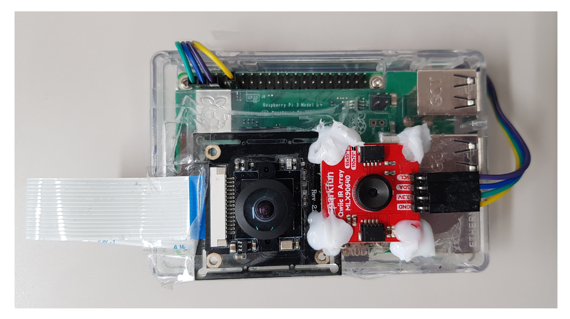
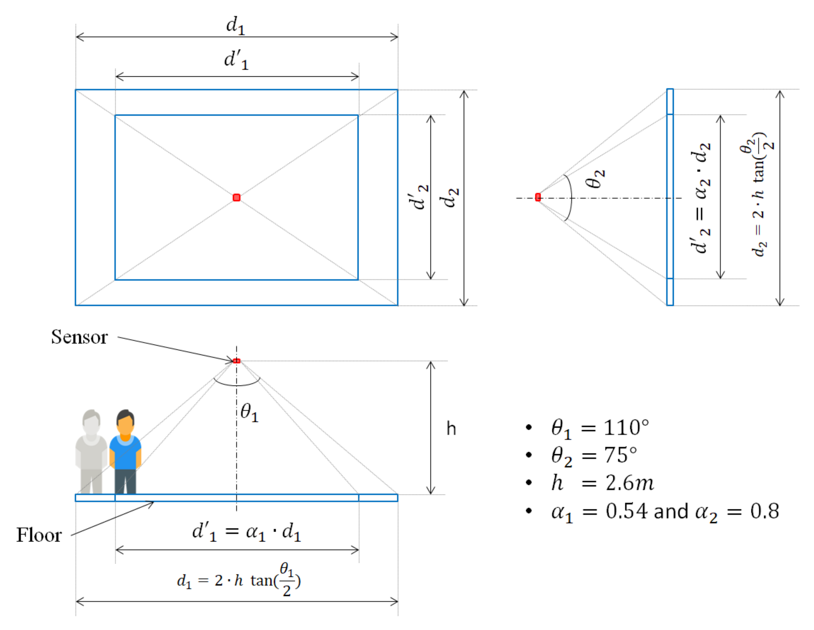
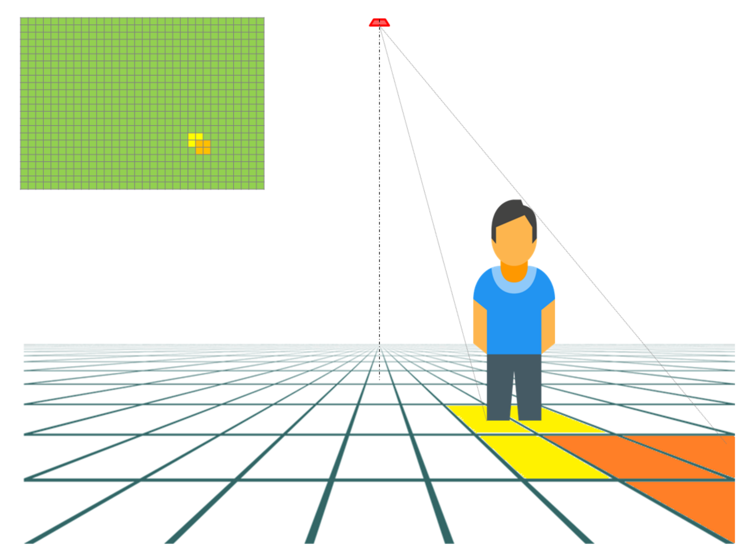
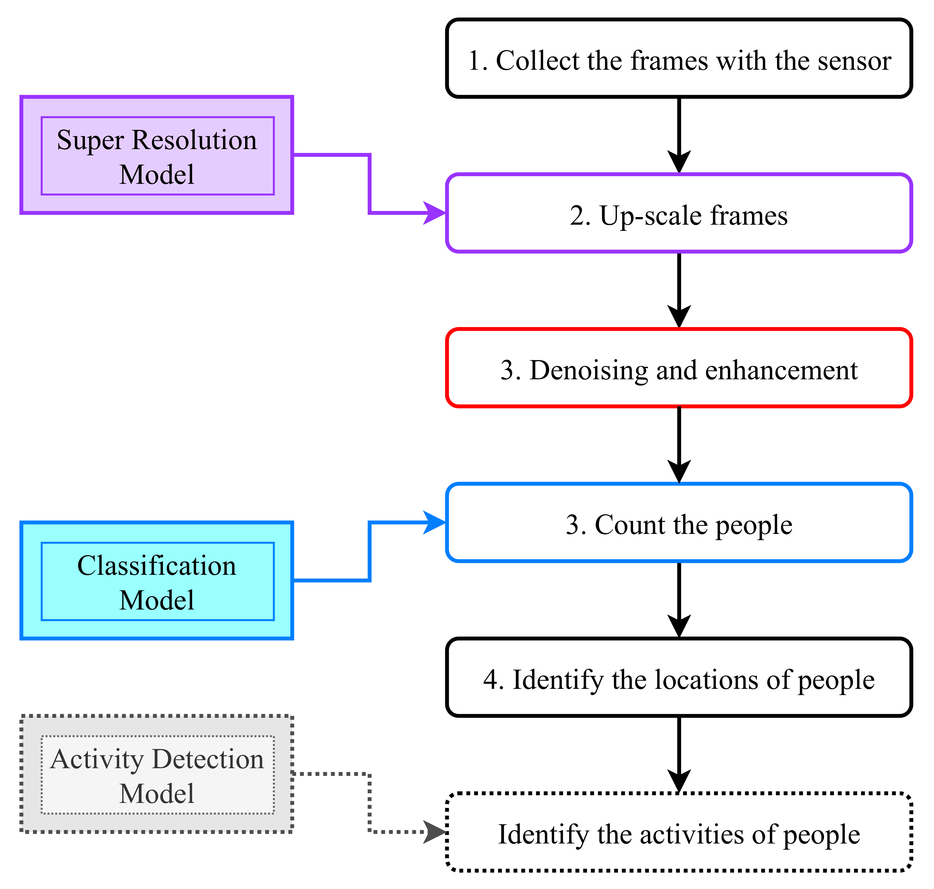
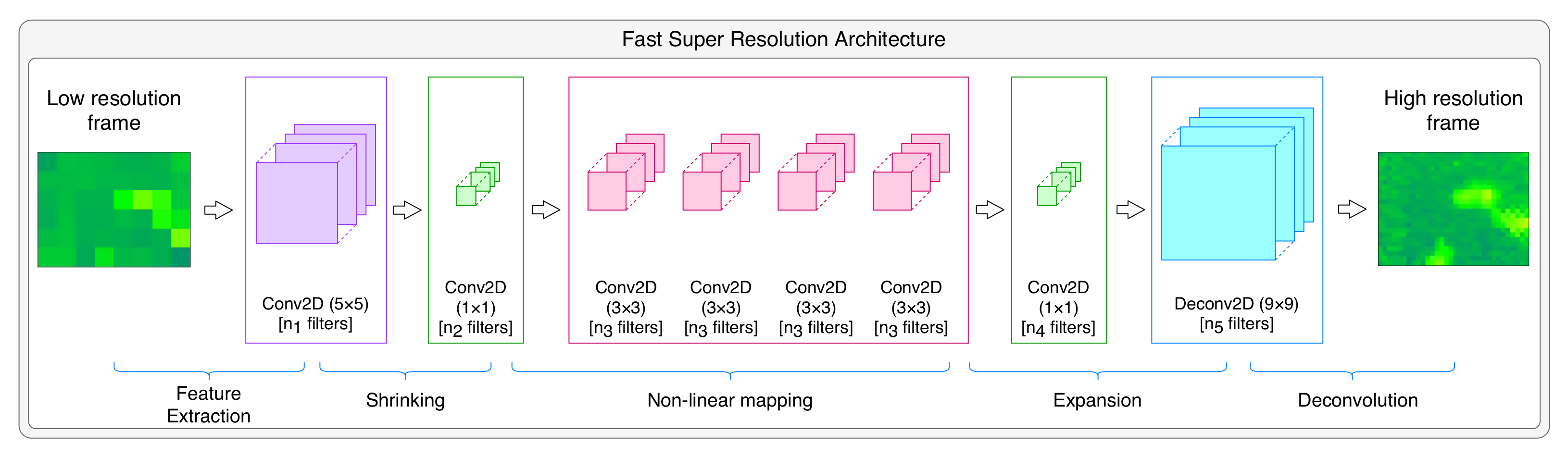
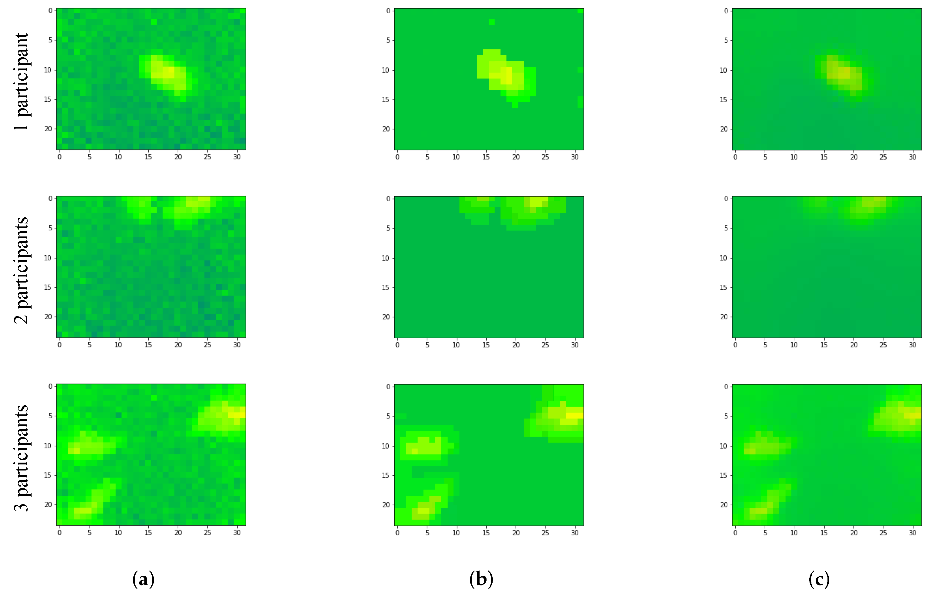

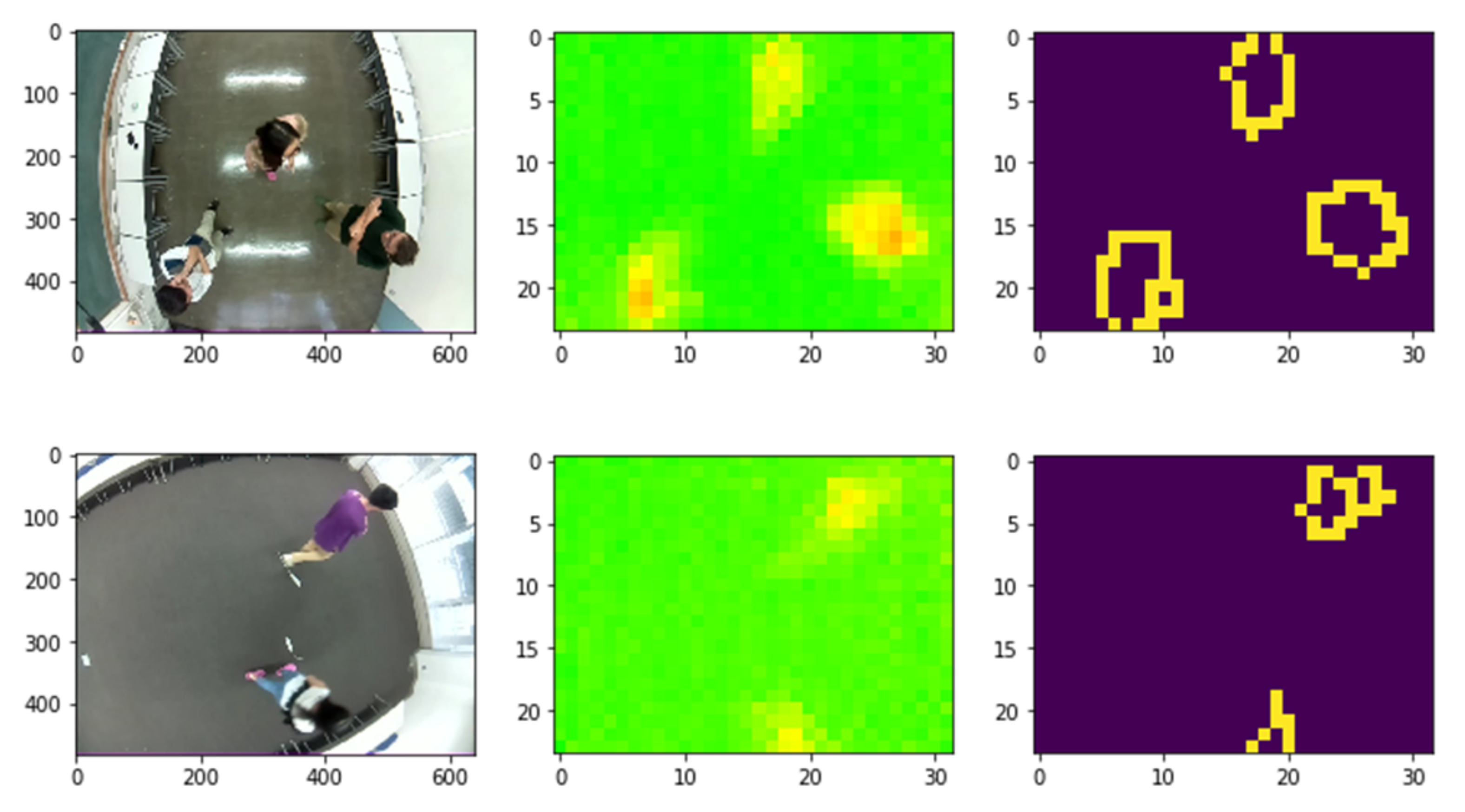
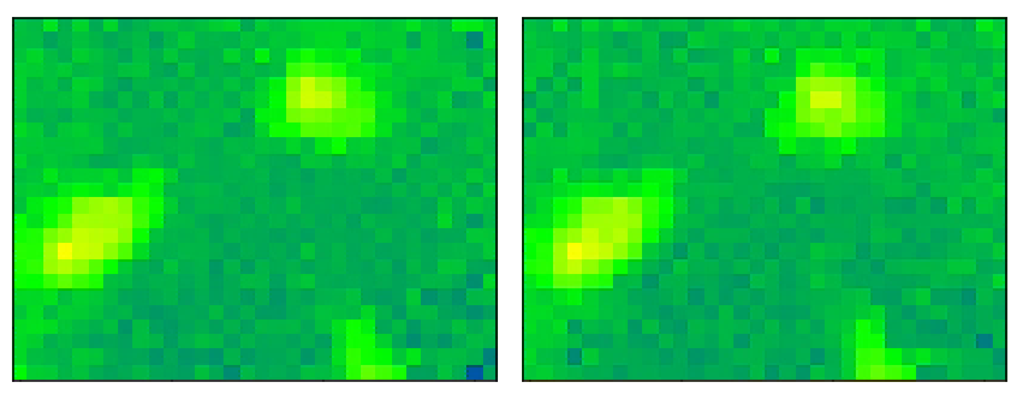

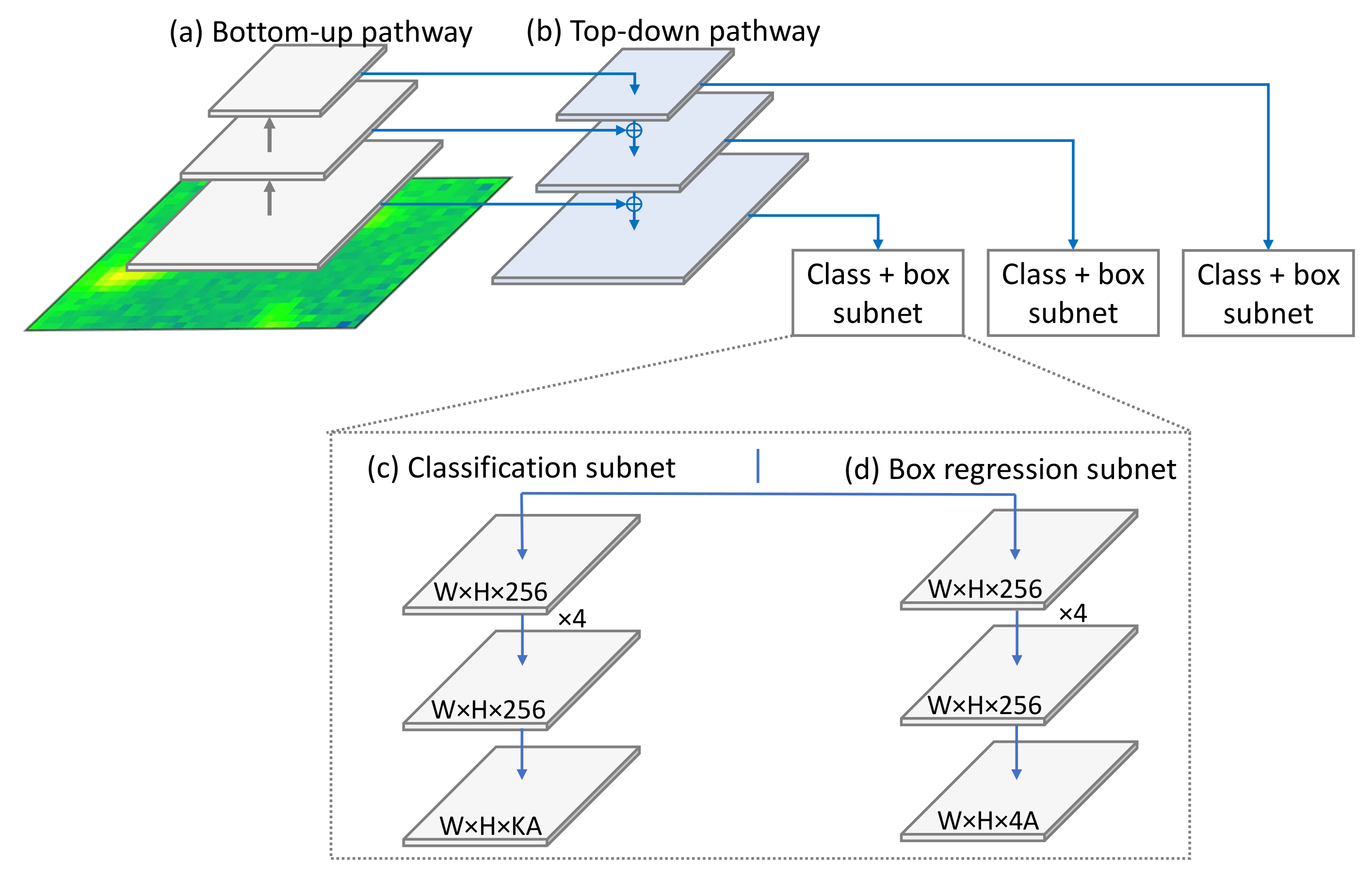
Publisher’s Note: MDPI stays neutral with regard to jurisdictional claims in published maps and institutional affiliations. |
© 2022 by the authors. Licensee MDPI, Basel, Switzerland. This article is an open access article distributed under the terms and conditions of the Creative Commons Attribution (CC BY) license (https://creativecommons.org/licenses/by/4.0/).