Abstract
Medical images of brain tumors are critical for characterizing the pathology of tumors and early diagnosis. There are multiple modalities for medical images of brain tumors. Fusing the unique features of each modality of the magnetic resonance imaging (MRI) scans can accurately determine the nature of brain tumors. The current genetic analysis approach is time-consuming and requires surgical extraction of brain tissue samples. Accurate classification of multi-modal brain tumor images can speed up the detection process and alleviate patient suffering. Medical image fusion refers to effectively merging the significant information of multiple source images of the same tissue into one image, which will carry abundant information for diagnosis. This paper proposes a novel attentive deep-learning-based classification model that integrates multi-modal feature aggregation, lite attention mechanism, separable embedding, and modal-wise shortcuts for performance improvement. We evaluate our model on the RSNA-MICCAI dataset, a scenario-specific medical image dataset, and demonstrate that the proposed method outperforms the state-of-the-art (SOTA) by around 3%.
1. Introduction
GLOBOCAN recently conducted a survey in 185 countries, reporting an estimation of over 300 K new brain cancer cases and above 250 K new deaths in 2020 [1]. Among the various types of malignant brain tumors, glioblastoma multiforme (GBM) is one of the most deadly types, with a low survival rate and limited treatment options. In the United States, the estimated number of GBM diagnoses is over 13 K, and the number of deaths resulting from GBM is over 10 K per year [2]. GBM has been classified as the highest-grade brain cancer (a grade five) by the World Health Organization. A combination of chemotherapy and radiotherapy is a typical treatment following the removal of the tumor by surgery. Radiotherapy can cause severe side effects since radiation could kill both normal and cancer cells. Chemotherapy, on the other hand, works by placing a chemical on the guanine DNA, preventing the replicating of new DNA and leading to cancer cell apoptosis. However, it is known that chemotherapy can be ineffective due to an enzyme named O-methylguanine DNA methyltransferase (MGMT). The function of MGMT is determined by its promoter methylation status. If the promoter region is methylated, the enzyme transcription is affected, leading to potentially effective chemotherapy treatment. Therefore, the MGMT promoter methylation status has become a prognostic factor, and a predictor of chemotherapy response [3].
Invasive surgeries can be utilized to determine the status of the MGMT promoter methylation. However, this approach, based on genetic analysis, is an iterative and time-consuming process that requires surgical extraction of brain tissue samples and several weeks of genetic characterization. In addition, the surgery itself may lead to side effects. An alternative that does not involve surgery is to apply computer vision techniques to analyze the magnetic resonance imaging (MRI) data. Recent advances in deep learning have achieved extensive success in a broad spectrum of domains [4]. With the continuous efforts of MRI data collection and annotation, deep learning shows its potential in MGMT promoter methylation detection by learning and extracting biomarkers and patterns from MIR scans that are highly indicative of the methylation status. Thus, deep-learning-based approaches have the potential to offer a non-invasive, efficient, and accurate alternative with less patient suffering and more effective treatment for GBM.
MRI scans contain abundant data with a characteristic of multi-modality, which can be and should be better exploited by deep learning algorithms. However, our investigation of the literature shows that prior studies have not fully explored the usage of multi-modal MRI data to detect MGMT methylation. Among the several studies [5,6,7,8] that considered multi-modality, only a basic fusion strategy has been adopted, and there is a lack of in-depth investigation for utilizing the multi-modality feature of MRI data for brain tumor detection. Our study aims to fill this gap.
In this paper, we propose a novel deep neural network (DNN) architecture that integrates three performance boosters, including a lite attention mechanism, a separable embedding module, and a model-wise shortcut strategy. The three boosters are designed to better mine multi-modal features and capture informative patterns to make a final prediction. Our proposed model is lightweight and can effectively improve the model performance. The main contributions of this study are as follows.
- We propose an attentive multi-modal DNN to predict the status of the MGMT promoter methylation. In addition to a multi-modal feature aggregation strategy, our proposed model integrates three performance boosters, including a lite attention mechanism to control the model size and speed up training, a separable embedding module to improve the feature representation of MRI data, and a modal-wise shortcut strategy to ensure the modal specificity. These joint efforts have improved the detection accuracy of our model by 3%, compared to the SOTA method. Experiments and results are obtained on the RSNA-MICCAI 2021 dataset [9], which is a recently released dataset with the most patients and MRI scans compared to existing datasets.
- We have made the project source code publicly available at https://github.com/ruyiq/An-Attentive-Multi-modal-CNN-for-Brain-Tumor-Radiogenomic-Classification (accessed at 26 February 2020), offering a credible benchmark for future studies.
The rest of this paper is organized as follows. Section 2 reviews research work related to fusion of multi-modal medical images. Section 3 explains our proposed model and dataset. In Section 4, several experiments are conducted to evaluate the effectiveness of the proposed model. Finally, in Section 5 we conclude the paper and provide future work.
2. Related Work
2.1. Detection of MGMT Methylation Status Based on MRI Data
Table 1 lists a collection of learning-based methods trained with brain MRI scans for the classification of methylation status, which is usually treated as a binary classification problem; namely, methylation vs. non-methylation. It is observed that both traditional feature-based learning methods [5,10,11], such as SVM, RF, KNN, RF, J48, NB, and XGBoost, and deep learning models [6,7,8,12,13], such as CNN and RNN, have been extensively adopted to build classifiers. It is also noted that a lack of sufficient training data has been a long-lasting challenge, limiting the power of deep-learning-based models. Most prior studies have used data from the Cancer Genome Atlas (TCGA) database, which contains MRI scans from fewer than 250 patients. The recent 2021 RSNA-MICCAI dataset [9] has doubled the number of patients with data collected from multiple centers. This enhancement can boost the quantity and diversity of data used for training deep neural network (DNN) models in the area of methylation detection and potentially benefit the model performance. Meanwhile, it is essential to utilize MRI scans with different modalities, which provide more abundant image features and patterns to be learned by a model. It is found that only half of the studies [5,6,7,8] have considered the multi-modality characteristic of the data. We argue that the multi-modal image features play a crucial role in building a more accurate and robust model for MGMT methylation detection, which drives us to integrate a multi-modal feature fusion strategy into the learning pipeline. Moreover, we propose to adopt three performance boosters, including a lite attention mechanism, a modal-wise shortcut, and a separable embedding strategy, which have not been seen in prior studies.

Table 1.
A review of MRI-based learning models for the detection of MGMT methylation status. The table includes the following abbreviations: dataset size (D.S.), multi-modality (M.M.), attention mechanism (A.M.), modal-wise shortcut (M.W.S.), separable embedding (S.E.), support vector machine (SVM), random forest (RF), k-nearest neighbor (KNN), naive Bayes (NB), convolutional neural network (CNN), and deep neural network (DNN).
2.2. Multi-Modal Learning on MRI Data
It has been shown both theoretically [14] and empirically [15,16] that models aggregating data from multiple modalities outperform their uni-modal counterparts due to the enriched features and patterns to be learned from the multi-modal data. The usage of multi-modal learning has seen success in a wide range of learning tasks such as object detection [17], semantic segmentation [18], video action recognition [19], and detection of disease [20,21].
MRI data also present multiple modalities that can be extensively utilized for training DNN models. Several studies have developed various techniques to pursue better predictive performance. Myronenko et al. applied AutoEncoder, which fuses the inputs from different modalities [15] to achieve a better performance in 3D MRI brain tumor segmentation. Tseng et al. proposed a deep encoder–decoder structure with cross-modality convolution layers for 3D image segmentation [16]. Shachor et al. proposed an ensemble network architecture to address the classification task by fusing several data sources [22]. The designed network consists of three different modality-specific encoders to capture features of different levels. The proposed method focuses on two-view mammography, which could be extended to multiple views and/or multiple scans. Nie et al. proposed the use of fully convolutional networks (FCNs) for the segmentation of isointense phase brain MR images. They trained one network for each modality image and then fused their high-layer features for final segmentation, which uses different modality paths to obtain the modality-specific features and then fuses the features to make final decisions [23]. Kamnitsas et al. fused the input modality-wise information directly [24]. They proposed a dual pathway, 11-layer deep, 3-dimensional convolutional neural network for brain lesion segmentation. They also devised an efficient and effective dense training scheme, which joins the processing of adjacent image patches into one pass.
The aforementioned studies mainly use multi-modal MRI data to build DNN models for the segmentation task. To the best of our knowledge, the usage of multi-modal MRI data for the detection of MGMT methylation has not been seen. Moreover, the proposed learning pipeline integrates three performance boosters to utilize better the extracted multi-modal MRI features, which have not appeared in any prior studies we have investigated.
3. Materials and Methods
3.1. Dataset
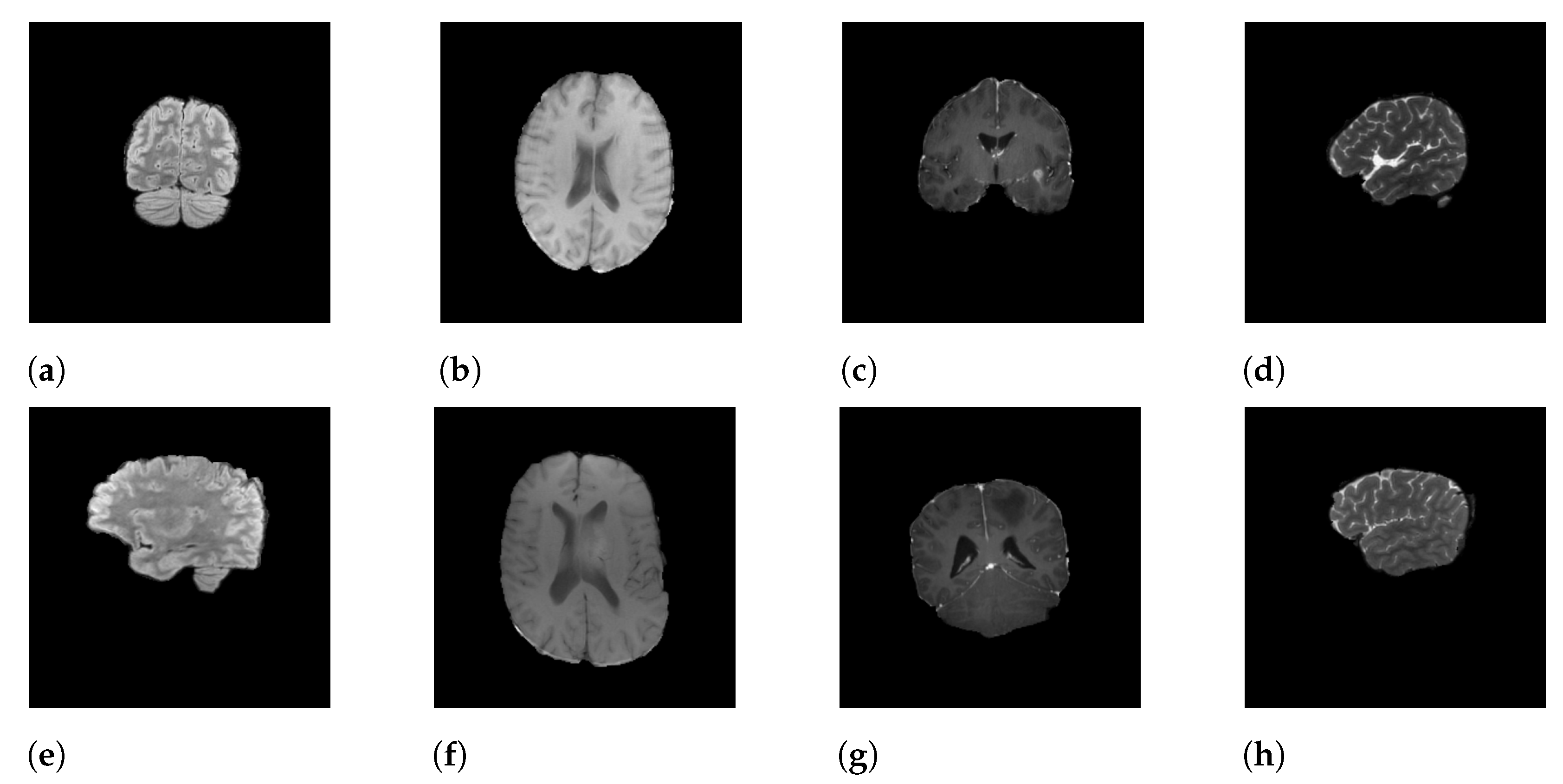
In this research, we focus on the RSNA-MICCAI dataset [9], a multi-center brain tumor MRI dataset that comes with two tasks; namely, tumor segmentation and MGMT detection. In this study, we only tackle the second one. In the dataset, each patient’s data is stored in a dedicated folder with a five-digit identification number. Each sample folder consists of four sub-folders corresponding to the four modalities of the MRI scans, including fluid attenuated inversion recovery (FLAIR), T1-weighted pre-contrast (T1w), T1-weighted post-contrast (T1Gd), and T2-weighted (T2), obtained from the video cut frames acquired by imaging. Each modality (i.e., scan type) specifies a focus during imaging. For instance, FLAIR captures the effect after cerebrospinal fluid (CSF) suppression, where liquid signals such as water are suppressed to highlight other parts. T2-weighted, on the other hand, highlights the difference in lateral tissue relaxation, and the combination of different effects provides a comprehensive description of the lesion from multiple perspectives. Each sample in the dataset is described by a quadruple of these four different imaging modalities. Figure 1 shows the four modalities of a positive sample (Figure 1a–d) and a negative sample (Figure 1e–h).

Figure 1.
Samples of MRI scans: (a–d) represent the FLAIR, T1w, T1Gd, and T2 modalities of a positive sample, and (e–h) represent the FLAIR, T1w, T1Gd, and T2 modalities of a negative sample.
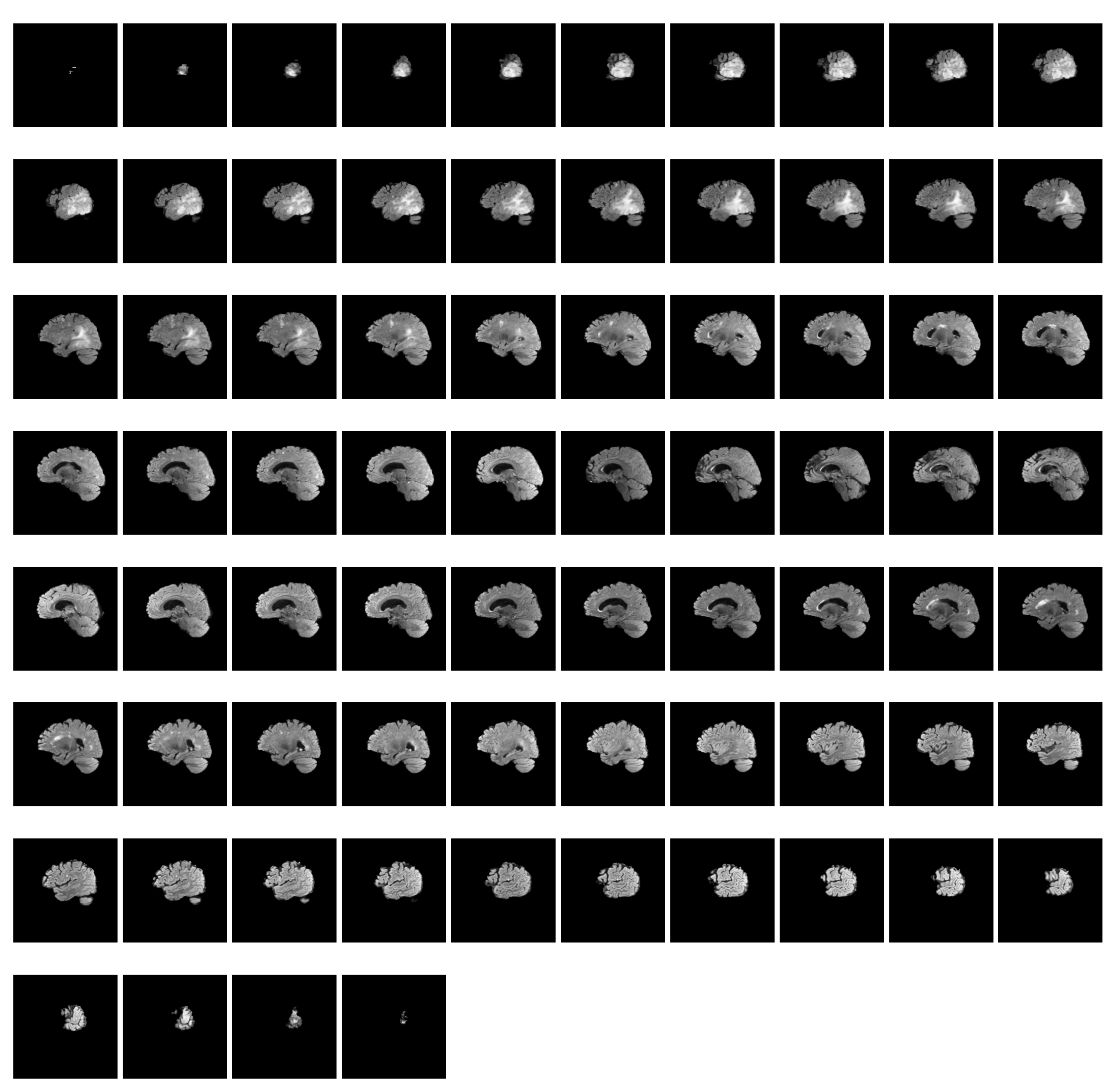
RSNA-MICCAI has 585 annotated samples, each corresponding to four modalities containing samples ranging from a few tens to a few hundred. Each modality of a patient consists of a sequence of MRI scans within a period of time. Figure 2 shows such an MRI sequence of FLAIR scans (74 in total) for patient ten in the dataset. Compared with other datasets used in prior studies in Table 1, RSNA-MICCAI contains a larger amount of data and is a clearly labeled dichotomous dataset, which can better characterize the patient in different imaging modalities and have better generalization. The number of positive MRI scans is 3070, or 57.5%, and the number of negative samples is 2780, or 52.5%. The classes of the dataset are relatively balanced. Table 2 reports the statistics of the number of MRI scans for each modality. It is observed that the average number of scans for modality per patient is in the range 127 and 171, which provides abundant information for pattern learning.

Figure 2.
A sequence of FLAIR scans for patient 10 in the dataset.
Table 2.
Number of files for each scan type.
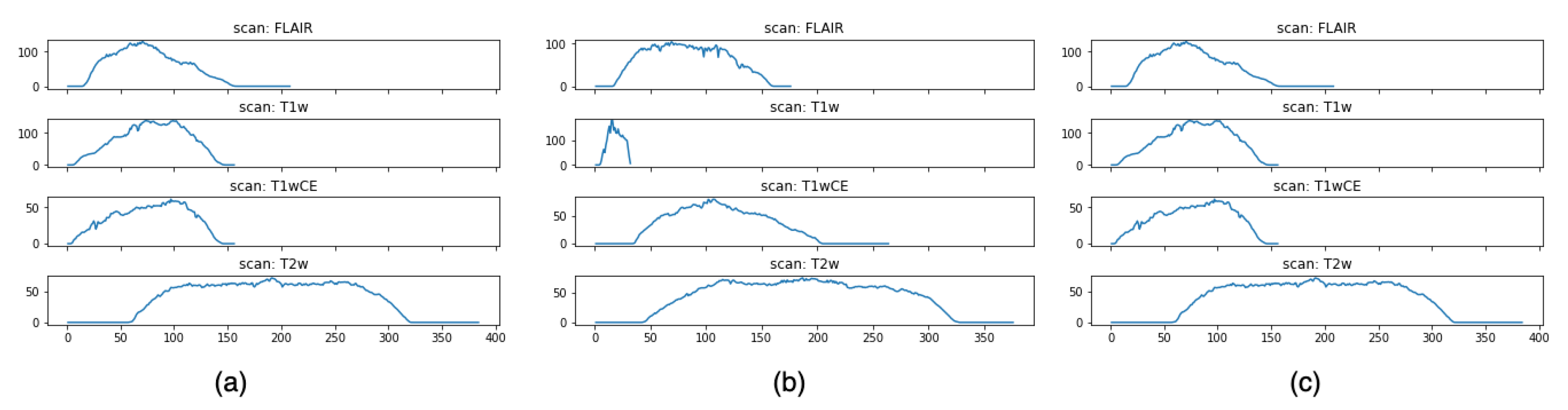
Figure 3 shows an intensity visualization of MRI scans for three random patients. The charts are grouped by the four modalities. For each sub-chart, the x-axis represents the time step, and the y-axis denotes an intensity score, which reflects the amount of information expressed by the MRI scan at a time step. The intensity defines the shade of gray of tissues or fluid, and different levels of intensity are encoded by different colors in the MRI scan. The higher the intensity, the more white area in the scan; the lower the intensity, the more black in the scan. Thus, gray encodes intermediate signal intensity. Intuitively, images with higher intensity carry more expressive patterns that can be learned, and these images often appear in the middle of the MRI sequence, as shown in Figure 2. It is also observed that even for the same patient, the times of peak intensity for the four modalities vary. This finding allows us to better pre-process the data by selecting the most informative scans (namely, the ones with the highest intensity scores) for each modality to train our model.
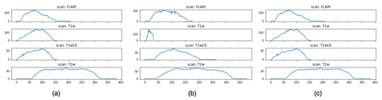
Figure 3.
Intensity visualization. Subfigures (a–c) represent the intensity charts of the four modalities for three randomly selected samples.
3.2. Learning Framework
Figure 4 illustrates the learning framework. To ensure the model effect and retain the original input details, the output of attention is fused with the input through shortcut connection and weighted summation, and the fused features are mapped to a more divisible space by a smaller DNN module. Finally, the classification results are obtained by using the LSTM structure. In this paper, four sub-structures, including multi-modal feature aggregation, lite attention mechanism, separable embedding, and modal-wise shortcut, are applied together to enhance the overall performance of classification.
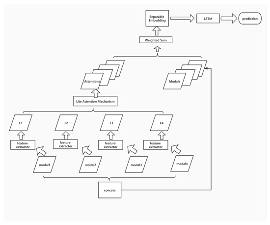
Figure 4.
The learning framework.
3.3. Multi-Modal Feature Fusion
The data of each modality are considered for modality-by-modality feature extraction due to the significant differences in imaging principles. Each sample corresponds to four images, namely fluid attenuated inversion recovery (FLAIR), T1-weighted pre-contrast (T1w), T1-weighted post-contrast (T1Gd), and T2-weighted (T2), corresponding to modal1, modal2, modal3, and modal4 inputs in the above figure.
The feature maps F1, F2, F3, and F4, obtained through feature extraction from each modality, are fused by the attention module to obtain the attentions that can fully describe the overall information across the modalities.
Here, the specific form of feature extractor needs to be selected. Since the images of each modality are 256*256 single-channel images with small scales, an overly complex feature extraction process will greatly destroy the original information and make the subsequent operation difficult. It is found that a simple single-layer convolution can be used to obtain a balance between extracting features and preserving the original information. Since the data of each modality have a different distribution, the feature extractor of each branch does not share the weights.
To extract information from multiple perspectives, the subsequent attention module still adopts the multi-head model. The number of heads is chosen to be 4, which is explained below in Section 3.5.
3.4. Lite Attention Mechanism
Since each sample has four modalities, the data of each modality have a different emphasis due to their different methods of acquisition. It is necessary to analyze each data characteristic to decide how to fuse features from different modalities. The two commonly used methods are as follows:
- Fuse multi-modal data in the form of sequences and use recurrent neural network (RNN) models for feature extraction. This operation requires traversing the input from the first time-step to the last one, which is computationally expensive [25]. Even though improved RNN variants such as LSTM [26] and GRU [27] can effectively reduce the difficulty of parameter updates in training, the sequential arrangement of different modal data introduces unnecessary sequential priors, which can force the model to learn an unreasonable one-way information flow while understanding the inter-modal relationships to fit the main features, affecting the effectiveness of feature extraction [28,29].
- Use the attention mechanism to fuse the features extracted from different modalities. Attention can easily obtain global feature information compared to the sequential models such as LSTM and GRU mentioned above, which can better obtain contextual relationships and obtain an overall understanding of the input.
The attention mechanism was first proposed by the Google machine translation team in 2017. It completely breaks away from the previous framework based on a recurrent neural network and dynamically extracts the feature part that it cares most for from each current input and fuses it to control the impact of all time-step features on the current output through different weights [30]. A brief description of the attention mechanism is given as follows. In each time step, the input obtained by the model consists of three parts: the current query, different feature values, and the corresponding keys of the features. The query is the object that the model needs for the current time-step, which may be a concrete input or an abstract representation of the features extracted in the previous step. To fully determine the important differences of features, an attention mechanism uses the dot product of the query and key to calculate the weights of corresponding features. At this point, the similarity between the query and key is measured by the dot product [31]. This way of calculating attention weights is called dot-product attention. As such, we obtain the following Equation (1) for calculation, where and are the input key and values. The query at this point is denoted as q.
When the length of the vector becomes longer, the scale of its dot product result also becomes larger. After the calculation through softmax, it reaches the saturation zone, making the gradient smaller, which is not conducive to the model optimization. Therefore, before performing softmax, the inner product value is divided by the square root of the length d, as shown in Equation (2).
After a further examination of the equations above, it can be found that to perform the dot product operation, the key used by the model, i.e., , and the query, i.e., q, need to have the same dimensionality. The additive attention method is proposed to perform the weight calculation on different occasions adequately. This method concatenates the input query of length u and the key of length k. The resulting (query, key) pair is fed into a feedforward neural network with a single hidden layer, and the value describing the degree of similarity between the two is obtained by the sigmoid function and used as the weight [32].
In the above dot-product attention process, to calculate the weight corresponding to the i-th input, two vectors of length d, query and , for the case of N time steps or N different modalities, the number of parameters to be retained and trained is . To fully guarantee the relative importance of different inputs, the specific value of d cannot be too small since it is challenging to train the model effectively in the case of insufficient data.
In this study, we propose a lite attention mechanism, which is a light weighted improvement of the original attention mechanism, by directly modeling the weights of different modalities, i.e., rewriting the attention formula to the following:
For the training process of , the number of parameters is reduced from to N, which significantly improves the training speed and generalization performance [33,34]. It does not cost much to train . We do not use a softmax function for normalization and nonlinear processing before the weighted summation but achieve better results. Our conjecture is that the simple scale variation corresponding to normalization can be adjusted by the subsequent DNN embedding, while the parameters corresponding to formally relative simpler binary classification problems can be directly derived by incorporating the relationship of nonlinear mapping into the model structure.
3.5. Modal-Wise Shortcut
The features of each modal, after feature extraction and processing by the attention modules, are represented with a highly task-relevant tensor, but the following fusion process leads to a loss of image details that may be informative to the task, which may further result in severe performance degradation for the prediction. Our solution is to add a shortcut between the original input and the output of the attention module; namely, a residual connection [4] for each modal. Bypassing all the convolution and weighted summation, we keep and pass all the original detailed features in the network without any loss, which significantly reduces the possibility of model degradation.
The feature map that is finally fed into the DNN embedding can be represented as follows:
where is the ith feature map generated by the lite attention mechanism module, while is the original input for the ith modal. Fusing these two, we obtain , the new feature representation of the ith modal. To ensure the feasibility of the operation, the number of feature maps output by multi-head attention is set to be the same as the number of modals; namely, four. This step is processed separately for each modal to avoid cross-modal information interference, and the final improvement fully demonstrates the effectiveness of this operation.
3.6. Separable Embedding
A prior study named CLDNN [35] shows that mapping and projecting the extracted features into a new separable space before feeding them into the detection head can effectively boost the model’s accuracy. Inspired by this empirical finding, we adopt a separable embedding strategy in our study. Specifically, a separate CNN is utilized again to fuse the tensor produced from the previous module. We have evaluated two CNN backbones to fill this role and report their effects in the next section. The output of this module is given as follows.
where refers to the CNN that performs separable embedding; and refer to the input and output tensors of this module.
3.7. LSTM and Detection Head
The output of the separable embedding for each time step is then collected to form a collection of sequential tensors ordered by the time step of the MRI scans. The tensor sequence is then fed into a long short-term memory (LSTM) network, followed by a fully connected layer and a sigmoid function layer as the detection head that outputs a value in [0,1], indicating the probability of MGMT promoter methylation.
4. Experiments and Results
All experiments were implemented using Python. The adopted deep learning framework is Pytorch 1.8.0. Experiments were run on a Windows workstation with an i7-10875h CPU and a GTX2080TI GPU. Ten quartets were extracted from each original sample in the RSNA-MICCAI dataset as a new dataset, and a total of 5850 samples were obtained. The training and test sets were randomly divided according to the ratio of 8:2.
4.1. Evaluation Metrics
The primary metric of RSNA-MICCAI is the accuracy of the classification. We need to accurately determine whether the input image is obtained from malignant brain tumor imaging. Under the current scenario, the model should enhance the classification of positive samples that threaten the lives of patients. At the same time, misclassifying a true negative sample as a positive sample can lead to unnecessary surgery and post-operative torment for the patient. We need to improve the accuracy of both situations. To optimize both objectives simultaneously, the accuracy rate is used as the evaluation metric. The model with minor misclassification and omission is chosen.
in which TP (true positive) is the number of true positive samples; TN (true negative) is the number of true negative samples; FP (false positive) represents the number of false positive samples; and FN (false negative) is the number of false negative samples.
4.2. Baseline
We consider the following baselines in this study.
- ResNet by He et al. [4] is an effort to understand how deepening a neural network can increase the expressiveness and the complexity of the network. It is found that for DNN, if a newly added layer can be treated as an identity function, the deepened network is as effective as the original one. This finding drives the development of the residual block, which adds a shortcut connection to the layer output before the activation function. The simple design allows a DNN to be trained more easily and efficiently. ResNet was the winning solution for the ImageNet Large-Scale Visual Recognition Challenge in 2015 and has been applied to numerous computer vision tasks with SOTA performance. Therefore, we consider ResNet a decent baseline. Our empirical result shows that ResNet34 presents the highest accuracy. We thus use ResNet34 to represent the baseline result.
- The EfficientNet [36] paper makes two major contributions. First, a simple and mobile-size neural architecture was proposed. Second, a compound-scaling method was proposed to increase the network size to achieve maximum performance gains. It is suggested that to pursue better performance, the key is to balance all three dimensions, including network depth, width, and resolution, during ConvNet scaling. Thus, the authors of EfficientNet adopted a global scaling factor to uniformly scale the depth, width, and resolution of the network. The scaling factor makes it possible to apply grid searching to find the parameters that lead to the best performance. EfficientNet offers a generic neural architecture optimization technique applied to existing CNNs such as ResNet. It has shown superior performance in numerous tasks with SOTA results, which is why we chose it as a strong baseline.
- The gold-medal-winning strategy was developed by Firas Baba, who open-sourced the code at https://github.com/FirasBaba/rsna-resnet10 (accessed at 24 January 2020). The final model of the winning team is a 3D CNN using the ResNet10 backbone with the following design choices: BCE Loss, Adam optimizer, 15 epochs, a learning rate of 0.00001 (from epoch 1 to 10) and 0.000005 (from epoch 10–15), image size 256 by 256, batch size 8. Each epoch took around 80 s on an RTX 3090. The author also reported the best central image trick, which is a strategy to select the biggest MRI scan that contains the largest brain cutaway view for training. In this study, we refer to the model developed by Firas Baba as the SOTA since it was in first place on the contest leader board.
4.3. Training Setting
The 3 × 3 convolution is used as the feature extractor for each modality, and each modality uses its own feature extractor to obtain different features without sharing weights. We choose Adam as the optimizer with a learning rate of 0.0001, and beta1 and beta2 values of 0.9 and 0.999, respectively. We set eps=1 × 10⁻⁸ to prevent the denominator from being 0. Other parameter configurations are weight decay to be 0, batch size to be 8, and binary cross-entropy with logits to be the loss function of the binary classification problem. Several hyperparameters, including the learning rate, the batch size, and eps are tuned via a five-fold cross validation to obtain the optimal values given a list of value choices for each hyperparameter.
We also choose albumentation for data augmentation for the training dataset, with the following configurations:
- Horizontal flip with a probability of 0.5;
- Random affine transformation configured as shift-limit = 0.0625, scale_limit = 0.1, rotate_limit = 10 with a probability of 0.5;
- Random contrast transformation with 0.5 probability.
4.4. Performance Evaluation
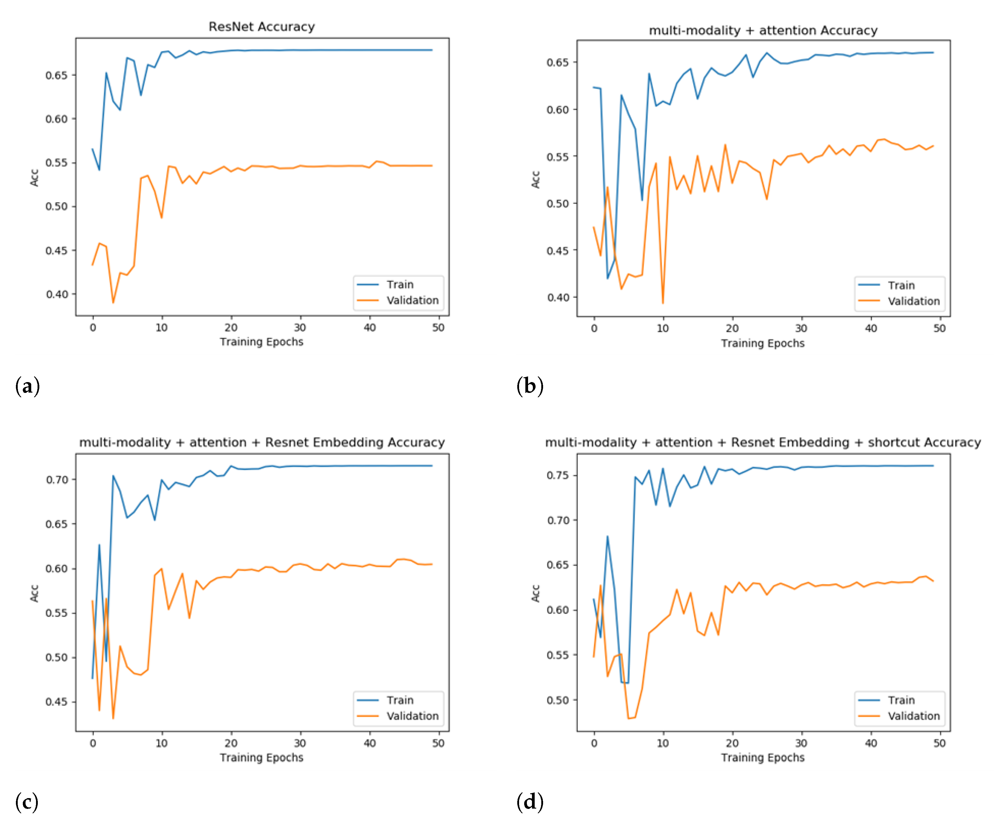
The accuracy of the evaluated models on the training set and the validation set is demonstrated in Figure 5. Under all configurations in this experiment, after 50 epochs of training, the models converge, and accuracy becomes stable.
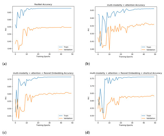
Figure 5.
Training and validation accuracy to show an ablation study. Subfigures (a–d) represent the four evaluated models with a booster added incrementally to the previous model.
Figure 5b shows the performance of adding the attention module only. The accuracy is only improved to 56.74%. However, the accuracy curve converges slower and a noticeable scale of oscillation appears in 20–30 epochs, which indicates that without adding other modules to the fusion of the extracted features the model is not able to obtain effective information. The training effect is poor, and the accuracy is not particularly satisfactory.
After adding two different separable embedding modules to the model, ResNet34 and EfficientNet [36], it can be observed that both accuracy and the convergence speed are greatly optimized, which fully illustrates the necessity of separable embedding. Specifically, the improvement of the performance by adding ResNet34 is more obvious and the convergence speed is also faster. The accuracy is improved by 4.35%, which is 61.09%. We chose ResNet34 as the separable embedding module for further experiments.
Finally, we added the shortcut model to the multi-modality + attention + Resnet34 embedding model, using weighted summation to fuse the original information and extracted features. It can be observed that adding the shortcut model further improves the metrics by more than 2%, reflecting the effect of direct-concatenation for training the model. The performance of different models and training plans is provided in Table 3. Overall, the strategy of multi-modality + attention + Resnet34 Embedding + shortcut largely outperforms the baseline. Combining the above four submodules substantially improves the accuracy by more than 10%, but the absence of any one of them brings about a significant metric degradation. We also replicated the SOTA model, which utilized a 3D CNN + ResNet10 neural architecture. The SOTA had an accuracy of 60.74%, which is 3-point worse than our model.
Table 3.
Performance of different models. Abbreviations: separable embedding (S.E.), training duration per epoch (T.D.P.E).
We also report the average training duration per epoch (T.D.P.E.) in the last column of Table 3. It is observed that the average T.D.P.E. for all models ranges from 52.3 to 79.3 s on our deep learning workstation. The training has been relatively efficient mainly due to the following: (1) the MRI scans have been down-scaled to 256 by 256 pixels and (2) the fast processing speed offered by the RTX 3090. It is also noted that the best performing model only added a reasonable amount of time compared to the SOTA (79.3 vs. 73.1), which validates the efficient design of the lightweight attention module.
It is observed in Figure 5a–d that overfitting occurs in all evaluated models. Our observation is aligned with other contest participants (see a post at https://www.kaggle.com/c/rsna-miccai-brain-tumor-radiogenomic-classification/discussion/281347 accessed at 20 February 2022). It is mentioned that many teams obtained higher training scores than validation scores. In machine learning, overfitting is mainly caused by the nature of data [37]. Specifically, the data points of training and test sets do not follow the same distribution. As such, the models trained on the training set have learned knowledge and patterns that do not apply well to the samples on the test set. For this study, the quantity of MRI scans is increased compared to prior datasets. However, most scans only contain a partial area of the brain, which does not offer many expressive patterns to be learned by a model. We adopted the following strategies to handle overfitting. First, we applied several data augmentation strategies to enhance the diversity of the dataset (see Section 4.3). Second, we conducted cross-validation to examine the robustness of model performance. Despite these efforts, a performance gap in the range 10–15% still exists between the training and validation accuracy scores, even for our best-performing model.
5. Conclusions
Malignancy analysis of brain tumors is crucial for the lives of patients and early prevention. For early screening and reducing patients’ suffering, accurate classification is needed. However, the effectiveness of existing models cannot be guaranteed. In this paper, we proposed a new classification model based on multi-modal feature aggregation, lite attention mechanism, separable embedding, and modal-wise shortcut. The combined effects of these boosters increased the prediction accuracy to 63.71% on the RSNA-MICCAI dataset, outperforming the SOTA by 3%.
This work has the following limitations, which also suggest future directions. First, our proposed method only considers the temporal association between same-modality data, while the relationship between different modality data is not examined. This inter-modality relation is worthy of further investigation. Second, in addition to the modal-wise attention used in this study, image-wise attention can also be considered since some critical areas of an MRI scan could carry informative patterns that should be learned and used to make a better prediction. Lastly, a joint model that handles tumor segmentation and MGMT detection is expected.
Author Contributions
Conceptualization and methodology, R.Q. and Z.X.; software, validation, and original draft preparation, R.Q.; review and editing, and supervision, Z.X. All authors have read and agreed to the published version of the manuscript.
Funding
This research received no external funding.
Institutional Review Board Statement
Not applicable.
Informed Consent Statement
Not applicable.
Data Availability Statement
The dataset supporting the conclusions of this article are available at https://www.kaggle.com/c/rsna-miccai-brain-tumor-radiogenomic-classification (accessed on 20 November 2021).
Conflicts of Interest
The authors declare no conflict of interest.
References
- Sung, H.; Ferlay, J.; Siegel, R.L.; Laversanne, M.; Soerjomataram, I.; Jemal, A.; Bray, F. Global cancer statistics 2020: Globocan estimates of incidence and mortality worldwide for 36 cancers in 185 countries. CA Cancer J. Clin. 2021, 71, 209–249. [Google Scholar] [CrossRef] [PubMed]
- Ostrom, Q.T.; Patil, N.; Cioffi, G.; Waite, K.; Kruchko, C.; Barnholtz-Sloan, J.S. CBTRUS statistical report: Primary brain and other central nervous system tumors diagnosed in the United States in 2013–2017. Neuro-Oncology 2020, 22, iv1–iv96. [Google Scholar] [CrossRef] [PubMed]
- Zhou, T.; Ruan, S.; Canu, S. A review: Deep learning for medical image segmentation using multi-modality fusion. Array 2019, 3–4, 100004. [Google Scholar] [CrossRef]
- He, K.; Zhang, X.; Ren, S.; Sun, J. Deep Residual Learning for Image Recognition. In Proceedings of the 2016 IEEE Conference on Computer Vision and Pattern Recognition, Las Vegas, NV, USA, 27–30 June 2016; Volume 30, pp. 770–778. [Google Scholar]
- Le, N.Q.K.; Do, D.T.; Chiu, F.Y.; Yapp, E.K.Y.; Yeh, H.Y.; Chen, C.Y. XGBoost Improves Classification of MGMT Promoter Methylation Status in IDH1 Wildtype Glioblastoma. J. Pers. Med. 2020, 10, 128. [Google Scholar] [CrossRef]
- Korfiatis, P.; Kline, T.L.; Lachance, D.H.; Parney, I.F.; Buckner, J.C.; Erickson, B.J. Residual Deep Convolutional Neural Network Predicts MGMT Methylation Status. J. Digit. Imaging 2017, 30, 622–628. [Google Scholar] [CrossRef] [PubMed]
- Li, Z.C.; Bai, H.; Sun, Q.; Li, Q.; Liu, L.; Zou, Y.; Chen, Y.; Liang, C.; Zheng, H. Multiregional radiomics features from multiparametric MRI for prediction of MGMT methylation status in glioblastoma multiforme: A multicentre study. Eur. Radiol. 2018, 28, 3640–3650. [Google Scholar] [CrossRef]
- Han, L.; Kamdar, M.R. MRI to MGMT: Predicting methylation status in glioblastoma patients using convolutional recurrent neural networks. In Pacific symposium on Biocomputing 2018, Proceedings of the Pacific Symposium, Coast, HI, USA, 3–7 January 2018; World Scientific: Singapore, 2018; pp. 331–342. [Google Scholar]
- Baid, U.; Ghodasara, S.; Mohan, S.; Bilello, M.; Calabrese, E.; Colak, E.; Farahani, K.; Kalpathy-Cramer, J.; Kitamura, F.C.; Pati, S.; et al. The rsna-asnr-miccai brats 2021 benchmark on brain tumor segmentation and radiogenomic classification. arXiv 2021, arXiv:2107.02314. [Google Scholar]
- Korfiatis, P.; Kline, T.L.; Coufalova, L.; Lachance, D.H.; Parney, I.F.; Carter, R.E.; Buckner, J.C.; Erickson, B.J. MRI texture features as biomarkers to predict MGMT methylation status in glioblastomas. Med. Phys. 2016, 43, 2835–2844. [Google Scholar] [CrossRef]
- Kanas, V.G.; Zacharaki, E.I.; Thomas, G.A.; Zinn, P.O.; Megalooikonomou, V.; Colen, R.R. Learning MRI-based classification models for MGMT methylation status prediction in glioblastoma. Comput. Methods Programs Biomed. 2017, 140, 249–257. [Google Scholar] [CrossRef]
- Chen, X.; Zeng, M.; Tong, Y.; Zhang, T.; Fu, Y.; Li, H.; Zhang, Z.; Cheng, Z.; Xu, X.; Yang, R.; et al. Automatic Prediction of MGMT Status in Glioblastoma via Deep Learning-Based MR Image Analysis. Biomed Res. Int. 2020, 2020, 9258649. [Google Scholar] [CrossRef]
- Yogananda, C.; Shah, B.R.; Nalawade, S.; Murugesan, G.; Yu, F.; Pinho, M.; Wagner, B.; Mickey, B.; Patel, T.R.; Fei, B.; et al. MRI-based deep-learning method for determining glioma MGMT promoter methylation status. Am. J. Neuroradiol. 2021, 42, 845–852. [Google Scholar] [CrossRef] [PubMed]
- Huang, Y.; Du, C.; Xue, Z.; Chen, X.; Zhao, H.; Huang, L. What Makes Multi-modal Learning Better than Single (Provably). Adv. Neural Inf. Process. Syst. 2021, 34. [Google Scholar]
- Myronenko, A. 3D MRI Brain Tumor Segmentation Using Autoencoder Regularization. In Proceedings of the International Conference on Medical Image Computing and Computer Assisted Intervention Workshop(MICCAI), Shenzhen, China, 13–17 October 2019; pp. 311–320. [Google Scholar] [CrossRef]
- Tseng, K.L.; Lin, Y.L.; Hsu, W.; Huang, C.Y. Joint Sequence Learning and Cross-Modality Convolution for 3D Biomedical Segmentation. In Proceedings of the IEEE Computer Society Conference on Computer Vision and Pattern Recognition (CVPR), Honolulu, HI, USA, 21–26 July 2017; pp. 311–320. [Google Scholar] [CrossRef] [Green Version]
- Wang, A.; Lu, J.; Cai, J.; Cham, T.J.; Wang, G. Large-margin multi-modal deep learning for RGB-D object recognition. IEEE Trans. Multimed. 2015, 17, 1887–1898. [Google Scholar] [CrossRef]
- Liu, W.; Luo, Z.; Cai, Y.; Yu, Y.; Ke, Y.; Junior, J.M.; Gonçalves, W.N.; Li, J. Adversarial unsupervised domain adaptation for 3D semantic segmentation with multi-modal learning. ISPRS J. Photogramm. Remote Sens. 2021, 176, 211–221. [Google Scholar] [CrossRef]
- Wang, Z.; She, Q.; Smolic, A. TEAM-Net: Multi-modal Learning for Video Action Recognition with Partial Decoding. arXiv 2021, arXiv:2110.08814. [Google Scholar]
- Ning, Z.; Xiao, Q.; Feng, Q.; Chen, W.; Zhang, Y. Relation-induced multi-modal shared representation learning for Alzheimer’s disease diagnosis. IEEE Trans. Med. Imaging 2021, 40, 1632–1645. [Google Scholar] [CrossRef]
- Rani, G.; Oza, M.G.; Dhaka, V.S.; Pradhan, N.; Verma, S.; Rodrigues, J.J. Applying deep learning-based multi-modal for detection of coronavirus. Multimed. Syst. 2021, 1–12. [Google Scholar] [CrossRef]
- Shachor, Y.; Greenspan, H.; Goldberger, J. A mixture of views network with applications to multi-view medical imaging. IEEE Trans. Med. Imaging 2020, 374, 1–9. [Google Scholar] [CrossRef]
- Nie, D.; Wang, L.; Gao, Y.; Shen, D. Fully convolutional networks for multi-modality isointense infant brain image segmentation. In Proceedings of the 2016 IEEE 13th International Symposium on Biomedical Imaging (ISBI), Prague, Czech Republic, 13–16 April 2016; pp. 1342–1345. [Google Scholar] [CrossRef] [Green Version]
- Kamnitsas, K.; Ledig, C.; Newcombe, V.F.; Simpson, J.P.; Kane, A.D.; Menon, D.K.; Rueckert, D.; Glocker, B. Efficient multi-scale 3D CNN with fully connected CRF for accurate brain lesion segmentation. Med. Image Anal. 2017, 36, 61–78. [Google Scholar] [CrossRef]
- Cho, K.; Merrienboer, B.V.; Gulcehre, C.; Bahdanau, D.; Bougares, F.; Schwenk, H.; Bengio, Y. Learning Phrase Representations using RNN Encoder-Decoder for Statistical Machine Translationn. Comput. Sci. Comput. Lang. 2014, 36, 61–78. [Google Scholar] [CrossRef]
- Sainath, T.N.; Vinyals, O.; Senior, A.; Sak, H. Convolutional, Long Short-Term Memory, fully connected Deep Neural Networks. In Proceedings of the 2015 IEEE International Conference on Acoustics, Speech and Signal Processing (ICASSP), South Brisbane, QLD, Australia, 19–24 April 2015. [Google Scholar] [CrossRef]
- Zaremba, W.; Sutskever, I.; Vinyals, O. Recurrent Neural Network Regularization. Neural Evol. Comput. 2014, arXiv:1409.2329. [Google Scholar]
- Bahdanau, D.; Cho, K.; Bengio, Y. Neural Machine Translation by Jointly Learning to Align and Translate. Comput. Sci. Comput. Lang. 2014, arXiv:1409.0473. [Google Scholar]
- Cho, K.; van Merrienboer, B.; Bahdanau, D.; Bengio, Y. On the properties of neural machine translation: Encoder-decoder approaches. Comput. Sci. Comput. Lang. 2014, arXiv:1409.1259. [Google Scholar]
- Vaswani, A.; Shazeer, N.; Parmar, N.; Uszkoreit, J.; Jones, L.; Gomez, A.N.; Kaiser, L.; Polosukhin, I. Attention is All you Need. In Proceedings of the Conference on Neural Information Processing Systems (NeurIPS), Red Hook, NY, USA, 4–9 December 2017; Volume 30, pp. 1–12. [Google Scholar]
- Devlin, J.; Chang, M.; Lee, K.; Toutanova, K. BERT: Pre-training of Deep Bidirectional Transformers for Language Understanding. arXiv 2018, arXiv:1810.04805. [Google Scholar]
- Lan, Z.; Chen, M.; Goodman, S.; Gimpel, K.; Sharma, P.; Soricut, R. ALBERT: A Lite BERT for Self-supervised Learning of Language Representations. Neural Evol. Comput. 2019, arXiv:1909.11942. [Google Scholar]
- Zhang, Z.; Hanand, X.; Liu, Z.; Jiang, X.; Sun, M.; Liu, Q. ERNIE: Enhanced Language Representation with Informative Entities. In Proceedings of the 57th Annual Meeting of the Association for Computational Linguistics, Florence, Italy, 28 July–2 August 2019. [Google Scholar]
- Liu, Y.; Ott, M.; Goyal, N.; Du, J.; Joshi, M.; Chen, D.; Levy, O.; Lewis, M.; Zettlemoyer, L.; Stoyanov, V. RoBERTa: A Robustly Optimized BERT Pretraining Approach. arXiv 2019, arXiv:1907.11692. [Google Scholar]
- Sainath, R.Z.C.T.; Parada, C. Feature Learning with Raw-Waveform CLDNNs for Voice Activity Detection; Interspeech: Baixas, France, 2016. [Google Scholar]
- Tan, M.; Le, Q.V. Efficientnet: Rethinking model scaling for convolutional neural networks. arXiv 2019, arXiv:1905.11946. [Google Scholar]
- Dietterich, T. Overfitting and undercomputing in machine learning. Acm Comput. Surv. (CSUR) 1995, 27, 326–327. [Google Scholar] [CrossRef]

Publisher’s Note: MDPI stays neutral with regard to jurisdictional claims in published maps and institutional affiliations. |
© 2022 by the authors. Licensee MDPI, Basel, Switzerland. This article is an open access article distributed under the terms and conditions of the Creative Commons Attribution (CC BY) license (https://creativecommons.org/licenses/by/4.0/).