
Context-Aware Collaborative Filtering Using Context Similarity: An Empirical Comparison


Abstract
:1. Introduction
- Using context similarity is one of the major solutions to alleviate the sparsity issue in CARS. In this paper, we summarize different approaches to measure the context similarity, and discuss existing CACF approaches using context similarity.
- We deliver an empirical comparison among these recommendation algorithms, including some classical CACF approaches that were proposed at the early stage, but not compared with any existing research, such as the Chen’s method [17] in 2005.
2. Related Work
2.1. Context-Aware Recommender Systems
2.2. Context-Aware Collaborative Filtering
2.3. Sparsity Issue in CARS
3. Preliminary: Collaborative Filtering
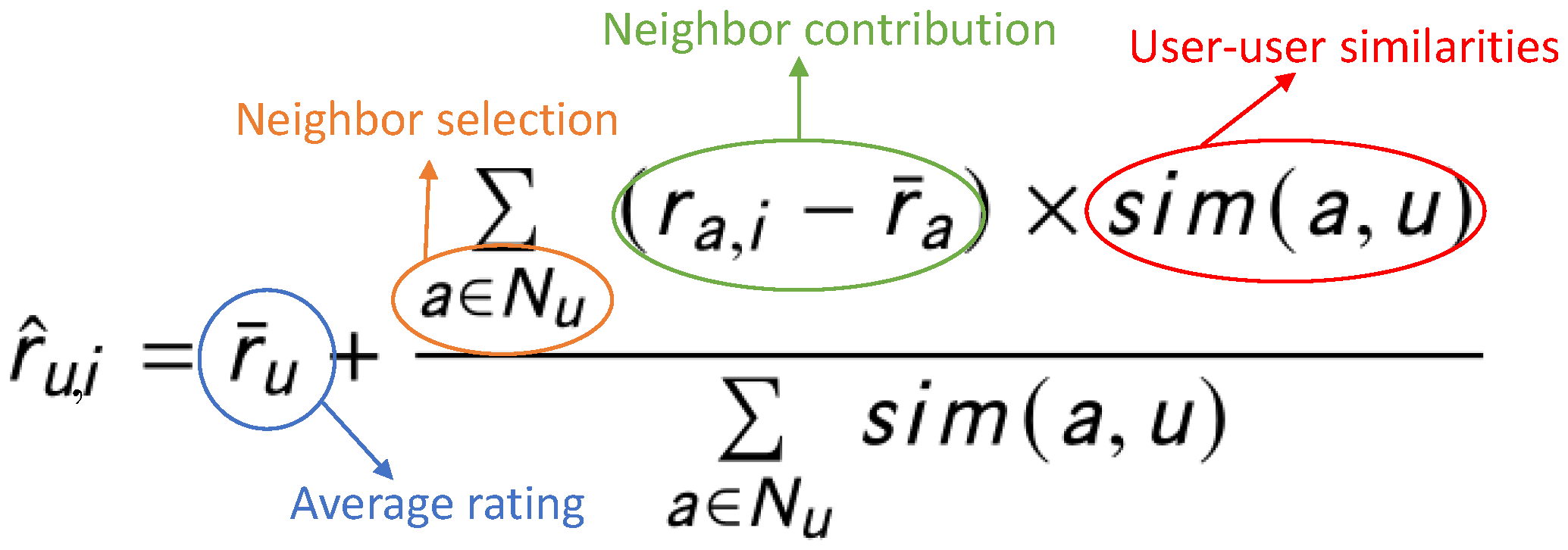
3.1. Memory-Based Collaborative Filtering
3.2. Model-Based Collaborative Filtering
4. Context-Aware Collaborative Filtering Using Context Similarity
4.1. Terminology and Notations
4.2. Semantic Similarity
4.3. Matching-Based Similarity
4.4. Inferred Similarity from Ratings
4.5. Learned Similarity Representations
4.6. Summary: Pros and Cons
5. Experiments and Results
5.1. Contextual Data Sets
- The Food data [50] was collected from surveys in which the subjects were asked to give ratings on Japanese food menus in two contextual dimensions: degree of hungriness in real situations, and degree of hungriness in assumed or imagined situations. Typical context conditions in these two dimensions are full, hungry, and normal. This is a good data set for exploring contextual preferences, since each user gave multiple ratings on a same item in different contexts.
- The Restaurant data [11] is also a data set collected from a survey. Subjects gave ratings to the popular restaurants in Tijuana, Mexico, by considering two contextual variables: time and location.
- The CoMoDa data [51] is a publicly available context-aware movie data collected from surveys. There are 12 context dimensions that captured users’ various situations, including mood, weather, time, location, companion, etc.
- The South Tyrol Suggests (STS) data [52] was collected from a mobile app that provides context-aware suggestions for attractions, events, public services, restaurants, and much more for South Tyrol. There are 14 contextual dimensions, such as budget, companion, daytime, mood, season, weather, etc.
- The Music data [53] was collected from InCarMusic, which is a mobile application (Android) offering music recommendations to the passengers of a car. Users are requested to enter ratings for some items using a web application. The contextual dimensions include driving style, road type, landscape, sleepiness, traffic conditions, mood, weather, and natural phenomena.
- The Frappe data [54] comes from the mobile usage in the app named Frappe, which is a context-aware app discovery tool that will recommend the right apps for the right moment. We used three context dimensions for experimental evaluations, including time of the day, day of the week, and location. This data captures the frequencies of an app used by each user within 2 months.
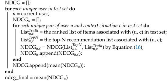
5.2. Evaluation Protocols
| Algorithm 1: Calculation of NDCG in CARS. |
 |
- CACF using context similarity.
- −
- Exact filtering (EF), which is the reduction approach proposed by Adomavicius et al. [7]. We use the contexts for exact filtering and apply MF in the remaining rating profiles to produce recommendations.
- −
- DCR uses the exact filtering on relaxed contexts, and DCW calculates context similarity based on a weighted matching. We present the results based on the non-dominated simplified DCR and DCW (i.e., noted by ND-DCR and ND-DCW), which are the latest variants of the DCR and DCW models mentioned in Section 4.3.
- −
- −
- SPF [10] and CBPF [42], which are two pre-filtering methods that rely on the context similarity based on the distributed vector representation for the context conditions. Note that CBPF runs slowly if there are several items and context conditions. The authors suggested to build the correlations on item clusters to speed up the computation process. We used K-Means clustering to build ten item clusters for the CoModa and Frappe data.
- −
- Context-aware matrix factorization using ICS, LCS, and MCS [38], which learns different similarity representations.
- Other CACF methods.
- −
- UISplitting [57], which is a pre-filtering model that combines user splitting and item splitting.
- −
- Context-aware matrix factorization (CAMF) [13], which learns a bias for each context condition. We use the version that assumes this bias is associated with an item. Namely, the bias for a same context condition may vary from items to items.
- −
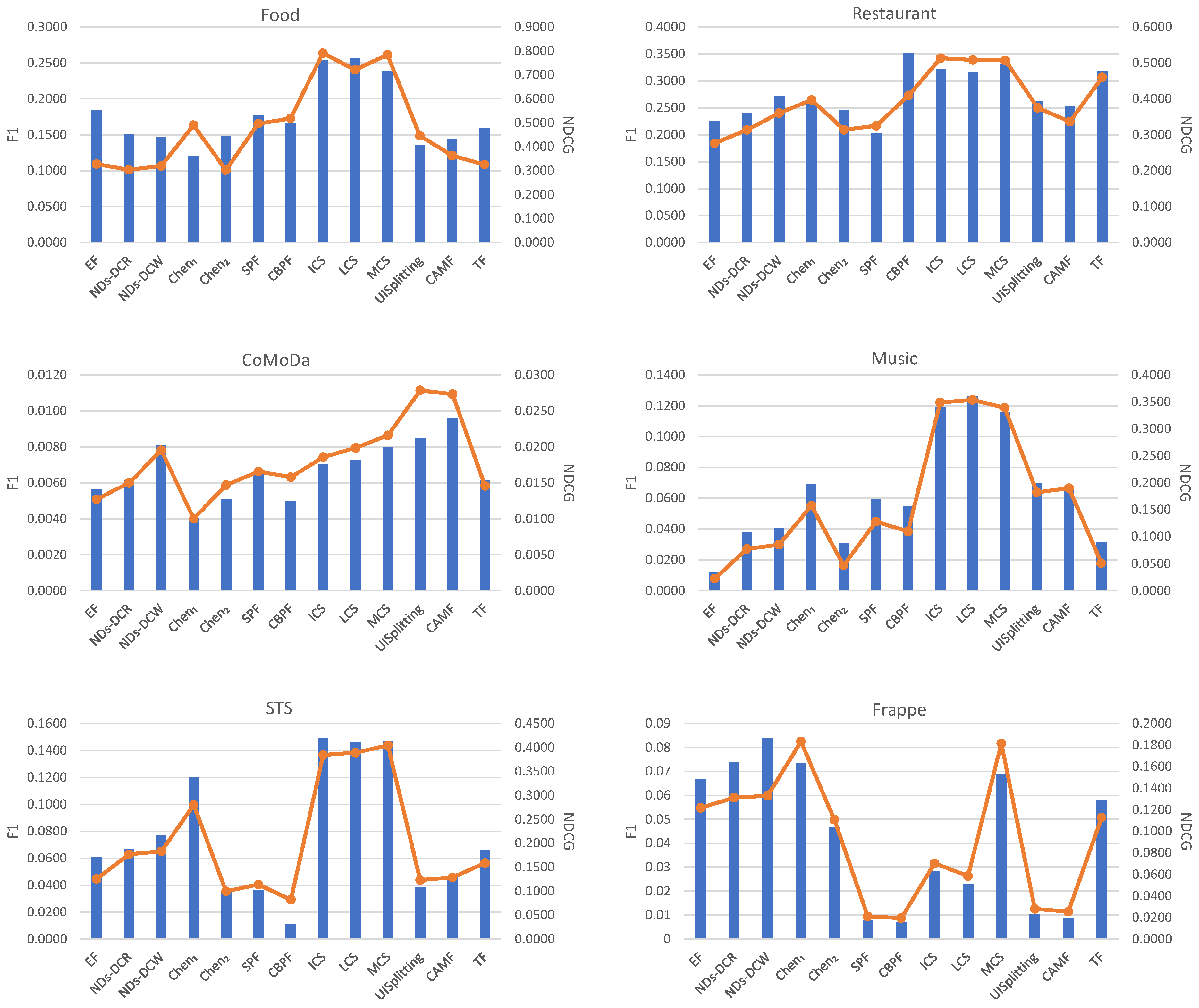
5.3. Results and Discussions
- Which one is the winner in terms of the comparison between CACF using context similarity and other CACF approaches?
- Which approach is the best among these CACF using context similarity?
- Among the three categories of CACF using context similarity (i.e., matching-based similarity, inferred similarity, learned similarity), which method is the best in each category?
5.3.1. Performance on Rating Predictions
5.3.2. Performance on Top-10 Recommendations
6. Conclusions and Future Work
Funding
Institutional Review Board Statement
Informed Consent Statement
Data Availability Statement
Conflicts of Interest
References
- Gross, B.M. The Managing of Organizations: The Administrative Struggle; JSTOR: New York, NY, USA, 1964; Volumes I and II. [Google Scholar]
- Ruff, J. Information Overload: Causes, Symptoms and Solutions; Harvard Graduate School of Education: Cambridge, MA, USA, 2002; pp. 1–13. [Google Scholar]
- Resnick, P.; Iacovou, N.; Suchak, M.; Bergstrom, P.; Riedl, J. GroupLens: An open architecture for collaborative filtering of netnews. In Proceedings of the 1994 ACM Conference on Computer Supported Cooperative Work, Chapel Hill, NC, USA, 22–26 October 1994; pp. 175–186. [Google Scholar]
- Koren, Y.; Bell, R.; Volinsky, C. Matrix factorization techniques for recommender systems. IEEE Comput. 2009, 42, 30–37. [Google Scholar] [CrossRef]
- Lops, P.; De Gemmis, M.; Semeraro, G. Content-based recommender systems: State of the art and trends. In Recommender Systems Handbook; Springer: New York, NY, USA, 2011; pp. 73–105. [Google Scholar]
- Burke, R. Hybrid Recommender Systems: Survey and Experiments. User Model. User-Adapt. Interact. 2002, 12, 331–370. [Google Scholar] [CrossRef]
- Adomavicius, G.; Sankaranarayanan, R.; Sen, S.; Tuzhilin, A. Incorporating contextual information in recommender systems using a multidimensional approach. ACM Trans. Inf. Syst. (TOIS) 2005, 23, 103–145. [Google Scholar] [CrossRef] [Green Version]
- Adomavicius, G.; Mobasher, B.; Ricci, F.; Tuzhilin, A. Context-Aware Recommender Systems. AI Mag. 2011, 32, 67–80. [Google Scholar]
- Baltrunas, L.; Ricci, F. Context-based splitting of item ratings in collaborative filtering. In Proceedings of the ACM Conference on Recommender Systems, New York, NY, USA, 23–25 October 2009; pp. 245–248. [Google Scholar]
- Codina, V.; Ricci, F.; Ceccaroni, L. Distributional semantic pre-filtering in context-aware recommender systems. User Model. User-Adapt. Interact. 2016, 26, 1–32. [Google Scholar] [CrossRef]
- Ramirez-Garcia, X.; Garcia-Valdez, M. Post-filtering for a restaurant context-aware recommender system. In Recent Advances on Hybrid Approaches for Designing Intelligent Systems; Springer: New York, NY, USA, 2014; pp. 695–707. [Google Scholar]
- Zheng, Y. Context-Aware Mobile Recommendation by a Novel Post-Filtering Approach. In Proceedings of the FLAIRS Conference, Melbourne, FL, USA, 21–23 May 2018; pp. 482–485. [Google Scholar]
- Baltrunas, L.; Ludwig, B.; Ricci, F. Matrix factorization techniques for context aware recommendation. In Proceedings of the Fifth ACM Conference on Recommender Systems, Chicago, IL, USA, 23–27 October 2011; pp. 301–304. [Google Scholar]
- Karatzoglou, A.; Amatriain, X.; Baltrunas, L.; Oliver, N. Multiverse recommendation: N-dimensional tensor factorization for context-aware collaborative filtering. In Proceedings of the Fourth ACM Conference on Recommender Systems, Barcelona, Spain, 26–30 September 2010; pp. 79–86. [Google Scholar]
- Zheng, Y.; Mobasher, B.; Burke, R. Integrating context similarity with sparse linear recommendation model. In Proceedings of the International Conference on User Modeling, Adaptation, and Personalization, Dublin, Ireland, 29 June–3 July 2015; pp. 370–376. [Google Scholar]
- Zheng, Y. Interpreting Contextual Effects by Contextual Modeling In Recommender Systems. In Proceedings of the ACM CIKM, the Workshop on Interpretable Data Mining (IDM)—Bridging the Gap between Shallow and Deep Models, Singapore, 6–10 November 2017. [Google Scholar]
- Chen, A. Context-aware collaborative filtering system: Predicting the user’s preferences in ubiquitous computing. In Proceedings of the CHI’05 Extended Abstracts on Human Factors in Computing Systems, Portland, OR, USA, 2–7 April 2005; pp. 1110–1111. [Google Scholar]
- Abowd, G.D.; Dey, A.K.; Brown, P.J.; Davies, N.; Smith, M.; Steggles, P. Towards a better understanding of context and context-awareness. In Handheld and Ubiquitous Computing; Springer: New York, NY, USA, 1999; pp. 304–307. [Google Scholar]
- Hidasi, B.; Karatzoglou, A.; Baltrunas, L.; Tikk, D. Session-based recommendations with recurrent neural networks. arXiv 2015, arXiv:1511.06939. [Google Scholar]
- Jannach, D.; Mobasher, B.; Berkovsky, S. Research directions in session-based and sequential recommendation. User Model. User-Adapt. Interact. 2020, 30, 609–616. [Google Scholar] [CrossRef]
- El Yebdri, Z.; Benslimane, S.M.; Lahfa, F.; Barhamgi, M.; Benslimane, D. Context-aware recommender system using trust network. Computing 2021, 103, 1919–1937. [Google Scholar] [CrossRef]
- Chen, B.; Xie, H. A Context-Aware Collaborative Filtering Recommender System Based on GCNs. In Proceedings of the 2020 International Conference on Intelligent Transportation, Big Data & Smart City (ICITBS), Vientiane, Laos, 11–12 January 2020; pp. 703–706. [Google Scholar]
- Qassimi, S.; Hafidi, M.; Qazdar, A. Towards a folksonomy graph-based context-aware recommender system of annotated books. J. Big Data 2021, 8, 67. [Google Scholar] [CrossRef]
- Resnick, P.; Varian, H.R. Recommender systems. Commun. ACM 1997, 40, 56–58. [Google Scholar] [CrossRef]
- Burke, R. Knowledge-based recommender systems. Encycl. Libr. Inf. Syst. 2000, 69, 175–186. [Google Scholar]
- Adomavicius, G.; Tuzhilin, A. Context-aware recommender systems. In Recommender Systems Handbook; Springer: New York, NY, USA, 2011; pp. 217–253. [Google Scholar]
- Sarwar, B.; Karypis, G.; Konstan, J.; Riedl, J. Item-based collaborative filtering recommendation algorithms. In Proceedings of the 10th International Conference on World Wide Web, Hong Kong, China, 1–5 May 2001; pp. 285–295. [Google Scholar]
- Ning, X.; Karypis, G. SLIM: Sparse linear methods for top-n recommender systems. In Proceedings of the 2011 IEEE 11th International Conference on Data Mining, Vancouver, BC, Canada, 11 December 2011; pp. 497–506. [Google Scholar]
- Wu, D.; Shang, M.; Luo, X.; Wang, Z. An L1-and-L2-Norm-Oriented Latent Factor Model for Recommender Systems. IEEE Trans. Neural Netw. Learn. Syst. 2021, 1–14. [Google Scholar] [CrossRef] [PubMed]
- Zhang, S.; Yao, L.; Sun, A.; Tay, Y. Deep learning based recommender system: A survey and new perspectives. ACM Comput. Surv. (CSUR) 2019, 52, 1–38. [Google Scholar] [CrossRef] [Green Version]
- Unger, M.; Shapira, B.; Rokach, L.; Bar, A. Inferring contextual preferences using deep auto-encoding. In Proceedings of the 25th Conference on User Modeling, Adaptation and Personalization, Bratislava, Slovakia, 9–12 July 2017; pp. 221–229. [Google Scholar]
- Jhamb, Y.; Ebesu, T.; Fang, Y. Attentive contextual denoising autoencoder for recommendation. In Proceedings of the 2018 ACM SIGIR International Conference on Theory of Information Retrieval, Tianjin, China, 14–17 September 2018; pp. 27–34. [Google Scholar]
- Unger, M.; Tuzhilin, A.; Livne, A. Context-Aware Recommendations Based on Deep Learning Frameworks. ACM Trans. Manag. Inf. Syst. (TMIS) 2020, 11, 8. [Google Scholar] [CrossRef]
- Wasid, M.; Ali, R. Context Similarity Measurement Based on Genetic Algorithm for Improved Recommendations. In Applications of Soft Computing for the Web; Springer: New York, NY, USA, 2017; pp. 11–29. [Google Scholar]
- Dixit, V.S.; Jain, P. Proposed similarity measure using Bhattacharyya coefficient for context aware recommender system. J. Intell. Fuzzy Syst. 2019, 36, 3105–3117. [Google Scholar] [CrossRef]
- Huynh, H.X.; Phan, N.Q.; Pham, N.M.; Pham, V.H.; Abdel-Basset, M.; Ismail, M. Context-Similarity Collaborative Filtering Recommendation. IEEE Access 2020, 8, 33342–33351. [Google Scholar] [CrossRef]
- Shi, Y.; Larson, M.; Hanjalic, A. Mining contextual movie similarity with matrix factorization for context-aware recommendation. ACM Trans. Intell. Syst. Technol. (TIST) 2013, 4, 16. [Google Scholar] [CrossRef]
- Zheng, Y.; Mobasher, B.; Burke, R. Similarity-based context-aware recommendation. In Proceedings of the International Conference on Web Information Systems Engineering, Miami, FL, USA, 1–3 November 2015; pp. 431–447. [Google Scholar]
- Liu, L.; Lecue, F.; Mehandjiev, N.; Xu, L. Using context similarity for service recommendation. In Proceedings of the 2010 IEEE Fourth International Conference on Semantic Computing, Pittsburgh, PA, USA, 22–24 September 2010; pp. 277–284. [Google Scholar]
- Zheng, Y.; Burke, R.; Mobasher, B. Optimal Feature Selection for Context-Aware Recommendation Using Differential Relaxation. Available online: https://citeseerx.ist.psu.edu/viewdoc/download?doi=10.1.1.416.4093&rep=rep1&type=pdf (accessed on 20 November 2021).
- Zheng, Y.; Burke, R.; Mobasher, B. Recommendation with differential context weighting. In Proceedings of the International Conference on User Modeling, Adaptation, and Personalization, Rome, Italy, 10–14 June 2013; pp. 152–164. [Google Scholar]
- Ferdousi, Z.V.; Colazzo, D.; Negre, E. Correlation-based pre-filtering for context-aware recommendation. In Proceedings of the 2018 IEEE International Conference on Pervasive Computing and Communications Workshops (PerCom Workshops), Athens, Greece, 19–23 March 2018; pp. 89–94. [Google Scholar]
- Kolahkaj, M.; Harounabadi, A.; Nikravanshalmani, A.; Chinipardaz, R. A hybrid context-aware approach for e-tourism package recommendation based on asymmetric similarity measurement and sequential pattern mining. Electron. Commer. Res. Appl. 2020, 42, 100978. [Google Scholar] [CrossRef]
- Zheng, Y. Non-Dominated Differential Context Modeling for Context-Aware Recommendations. Appl. Intell. 2022, 1–14. [Google Scholar] [CrossRef]
- Gupta, A.; Gusain, K. Selection of Similarity Function for Context-Aware Recommendation Systems. In Computational Intelligence in Data Mining; Springer: New York, NY, USA, 2017; pp. 803–811. [Google Scholar]
- Linda, S.; Minz, S.; Bharadwaj, K. Effective Context-Aware Recommendations Based on Context Weighting Using Genetic Algorithm and Alleviating Data Sparsity. Appl. Artif. Intell. 2020, 34, 730–753. [Google Scholar] [CrossRef]
- Kennedy, J.; Eberhart, R. A discrete binary version of the particle swarm algorithm. In Proceedings of the 1997 IEEE International Conference on Systems, Man, and Cybernetics, Computational Cybernetics and Simulation, Orlando, FL, USA, 12–15 October 1997; Volume 5, pp. 4104–4108. [Google Scholar]
- Kennedy, J.; Eberhart, R. Particle swarm optimization. In Proceedings of the ICNN’95—International Conference on Neural Networks, Perth, WA, Australia, 27 November–1 December 1995; Volume 4, pp. 1942–1948. [Google Scholar]
- Eshelman, L.J.; Schaffer, J.D. Real-coded genetic algorithms and interval-schemata. In Foundations of Genetic Algorithms; Elsevier: Amsterdam, The Netherlands, 1993; Volume 2, pp. 187–202. [Google Scholar]
- Ono, C.; Takishima, Y.; Motomura, Y.; Asoh, H. Context-Aware Preference Model Based on a Study of Difference between Real and Supposed Situation Data. In Proceedings of the International Conference on User Modeling, Adaptation, and Personalization, Trento, Italy, 22–26 June 2009; pp. 102–113. [Google Scholar]
- Košir, A.; Odic, A.; Kunaver, M.; Tkalcic, M.; Tasic, J.F. Database for contextual personalization. Elektrotehniski Vestn. 2011, 78, 270–274. [Google Scholar]
- Braunhofer, M.; Elahi, M.; Ricci, F.; Schievenin, T. Context-Aware Points of Interest Suggestion with Dynamic Weather Data Management. In Information and Communication Technologies in Tourism 2014; Springer: New York, NY, USA, 2013; pp. 87–100. [Google Scholar]
- Baltrunas, L.; Kaminskas, M.; Ludwig, B.; Moling, O.; Ricci, F.; Aydin, A.; Lüke, K.H.; Schwaiger, R. Incarmusic: Context-aware music recommendations in a car. In E-Commerce and Web Technologies; Springer: New York, NY, USA, 2011; pp. 89–100. [Google Scholar]
- Baltrunas, L.; Church, K.; Karatzoglou, A.; Oliver, N. Frappe: Understanding the Usage and Perception of Mobile App Recommendations In-The-Wild. arXiv 2015, arXiv:1505.03014. [Google Scholar]
- Zheng, Y.; Mobasher, B.; Burke, R. CARSKit: A Java-Based Context-aware Recommendation Engine. In Proceedings of the 15th IEEE International Conference on Data Mining Workshops, Atlantic City, NJ, USA, 14–17 November 2015. [Google Scholar]
- Järvelin, K.; Kekäläinen, J. Cumulated gain-based evaluation of IR techniques. ACM Trans. Inf. Syst. (TOIS) 2002, 20, 422–446. [Google Scholar] [CrossRef]
- Zheng, Y.; Burke, R.; Mobasher, B. Splitting approaches for context-aware recommendation: An empirical study. In Proceedings of the 29th Annual ACM Symposium on Applied Computing, Gyeongju, Korea, 24–28 March 2014; pp. 274–279. [Google Scholar]
- Harshman, R.A. Foundations of the PARAFAC Procedure: Models and Conditions for an “Explanatory” Multimodal Factor Analysis; University of California at Los Angeles: Los Angeles, CA, USA, 1970. [Google Scholar]


| References | Pre-Filtering | Contextual Modeling | NBCF | MF | |
|---|---|---|---|---|---|
| Semantic Similarity | Liu et al. [39] Kolahkaj et al. [43] | ✓ | ✓ | ||
| Matching-based Similarity | Adomavicius et al. [7], | ✓ | ✓ | ||
| Zheng et al. [40,41,44], Gupta et al. [45] Linda et al. [46] | ✓ | ✓ | |||
| Inffered Similarity from Ratings | Chen [17] | ✓ | ✓ | ||
| Codina et al. [10] Ferdousi, et al. [42] | ✓ | ✓ | |||
| Learned Similarity Representations | Zheng et al. [38] | ✓ | ✓ |
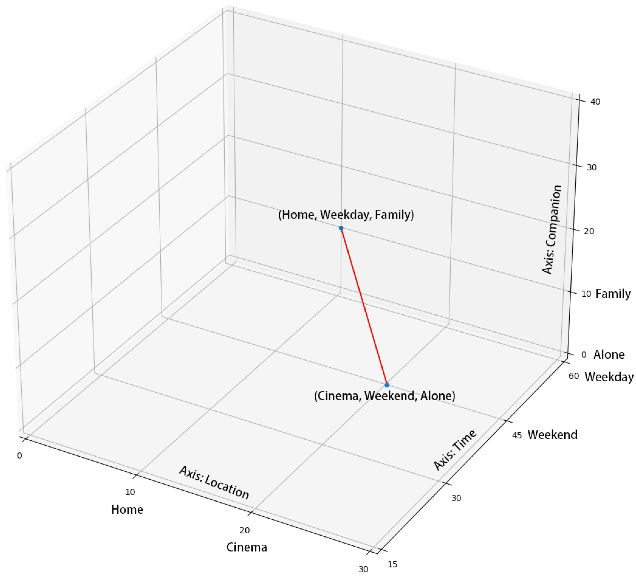
| User | Item | Rating | Time | Location | Companion |
|---|---|---|---|---|---|
| u | i | 3 | weekend | home | alone |
| u | i | 5 | weekend | cinema | partner |
| u | i | ? | weekday | home | family |
| Notation | Explanations |
|---|---|
| the number of users, items, and context dimensions, respectively, | |
| context situations | |
| a special context situation, with all dimensions as empty or N/A values. a non-contextual rating can be viewed as a rating in | |
| context conditions in the 1th, 2th, …, Zth dimension of the situation c | |
| rating given by user u on item i in context situation c | |
| rating given by user u on item i in context condition | |
| rating given by user u on item i without considering contexts | |
| , | training and testing set, respectively, |
| Food | Restaurant | CoMoDa | Music | STS | Frappe | |
|---|---|---|---|---|---|---|
| # of users | 212 | 50 | 121 | 42 | 325 | 957 |
| # of items | 20 | 40 | 1232 | 139 | 249 | 4082 |
| # of context dimensions | 2 | 2 | 8 | 5 | 11 | 3 |
| # of context conditions | 8 | 7 | 37 | 21 | 53 | 14 |
| # of ratings | 6360 | 2309 | 2292 | 3251 | 2354 | 87,580 |
| Rating scale | 1–5 | 1–5 | 1–5 | 1–5 | 1–5 | 0–4.46 |
| Density | 9.4% | 9.6% | 1.4 | 3.8 | 1.3 | 9.4 |
| Food | Restaurant | CoMoDa | Music | STS | Frappe | |
|---|---|---|---|---|---|---|
| EF | 0.900 | 1.026 | 0.833 | 1.165 | 0.961 | 0.409 |
| ND-DCR | 0.740 | 0.787 | 0.726 | 1.092 | 0.934 | 0.386 |
| ND-DCW | 0.725 * | 0.735 * | 0.726 * | 1.048 | 0.923 | 0.379 |
| Chen | 1.105 | 1.010 | 0.846 | 0.686 | 1.020 | 0.527 |
| Chen | 1.023 | 1.090 | 0.857 | 1.110 | 0.952 | 0.563 |
| SPF | 0.900 | 0.808 | 0.819 | 0.918 | 0.900 | 0.382 |
| CBPF | 1.068 | 0.972 | 0.830 | 1.110 | 1.060 | 0.402 |
| ICS | 0.858 | 0.825 | 0.777 | 0.678 | 0.986 | 0.388 |
| UISplitting | 0.805 | 0.813 | 0.775 | 0.657 | 0.893 | 0.378 |
| CAMF | 0.845 | 0.860 | 0.795 | 0.727 | 1.019 | 0.398 |
| TF | 0.966 | 0.945 | 0.858 | 0.864 | 0.916 | 0.392 |
Publisher’s Note: MDPI stays neutral with regard to jurisdictional claims in published maps and institutional affiliations. |
© 2022 by the author. Licensee MDPI, Basel, Switzerland. This article is an open access article distributed under the terms and conditions of the Creative Commons Attribution (CC BY) license (https://creativecommons.org/licenses/by/4.0/).
Share and Cite
Zheng, Y. Context-Aware Collaborative Filtering Using Context Similarity: An Empirical Comparison. Information 2022, 13, 42. https://doi.org/10.3390/info13010042
Zheng Y. Context-Aware Collaborative Filtering Using Context Similarity: An Empirical Comparison. Information. 2022; 13(1):42. https://doi.org/10.3390/info13010042
Chicago/Turabian StyleZheng, Yong. 2022. "Context-Aware Collaborative Filtering Using Context Similarity: An Empirical Comparison" Information 13, no. 1: 42. https://doi.org/10.3390/info13010042
APA StyleZheng, Y. (2022). Context-Aware Collaborative Filtering Using Context Similarity: An Empirical Comparison. Information, 13(1), 42. https://doi.org/10.3390/info13010042