Abstract
With the development of handheld video capturing devices, video stabilization becomes increasingly important. The gyroscope-based video stabilization methods perform promising ability, since they can return more reliable three-dimensional (3D) camera rotation estimation, especially when there are many moving objects in scenes or there are serious motion blur or illumination changes. However, the gyroscope-based methods depend on the camera intrinsic parameters to execute video stabilization. Therefore, a self-calibrated spherical video stabilization method was proposed. It builds a virtual sphere, of which the spherical radius is calibrated automatically, and then projects each frame of the video to the sphere. Through the inverse rotation of the spherical image according to the rotation jitter component, the dependence on the camera intrinsic parameters is relaxed. The experimental results showed that the proposed method does not need to calibrate the camera and it can suppress the camera jitter by binding the gyroscope on the camera. Moreover, compared with other state-of-the-art methods, the proposed method can improve the peak signal-to-noise ratio, the structural similarity metric, the cropping ratio, the distortion score, and the stability score.
1. Introduction
In recent years, with the development and popularization of handheld cameras and mobile phones, videos have been widely used to record interesting and important moments. However, in the moving environment, due to the instability of the carrier, the captured video is often accompanied by different degrees of image jitter [1,2]. This kind of jittered video will not only reduce the quality of the video, resulting in poor perception, but also affect the subsequent processing of the video [3]. Therefore, video stabilization is significant.
The purpose of video stabilization is to suppress or weaken the impact of camera jitter on video quality and to satisfy people’s perception and subsequent processing in the future. The video stabilization method can be mainly divided into three categories, i.e., mechanical image stabilization technology, optical image stabilization technology, and electronic image stabilization technology [4,5,6]. Mechanical image stabilization detects the jitter of the camera platform through gyro sensors and other devices and then adjusts the servo system to stabilize the image [7]. Optical image stabilization uses active optical components to adaptively adjust the optical path to compensate the image motion caused by the shaking of the camera platform, so as to achieve the purpose of image stabilization [8]. Electronic image stabilization computes motion estimation between consecutive images, and then motion smoothing and motion compensation are performed on each frame of the video to obtain a stable video [9]. Although mechanical image stabilization and optical image stabilization obtain better performance, there are still some problems such as large volumes, inconvenient carrying, and high cost. Therefore, electronic image stabilization has become a research hotspot in video stabilization.
Generally, electronic image stabilization includes three stages: camera motion estimation, motion smoothing, and video motion compensation [10]. According to different camera motion estimation methods, video stabilization can be divided into vision-based methods and attitude-sensor-based methods [11]. Vision-based methods usually estimate camera motion based on image sequences. Most of the existing methods model the transformation between two consecutive frames as affine transformation or homography transformation. This transformation relationship cannot model parallax, and it will be affected by moving objects and illumination transformation in the real-world scene. Attitude-sensor-based methods mainly use gyroscopes to estimate the camera rotation. Compared with vision-based methods, they can return more reliable three-dimensional (3D) camera rotation estimation, especially when there are many moving objects in the scene or there are serious motion blur or illumination changes in the video. Jia et al. proposed a video motion smoothing method based on a pure 3D rotation motion model and camera intrinsic parameters, which smooths the rotation matrix through a Riemannian geometry on a manifold [12]. Yang et al. proposed a Kalman filter method on a Lie group manifold to realize video stabilization, used a gyroscope to obtain rotation components for smoothing and used an intrinsic parameter matrix to calculate rotation projection on two-dimensional (2D) image for motion compensation [13]. Zhou et al. proposed a video stabilization method based on an optical flow sensor, which obtains rotation information through a gyroscope and describes image rotation by rotation around the z axis [14]. After using a gyroscope to compensate rotation jitter, Zhuang et al. used visual information to estimate the residual 2D translation in the image plane [15]. The premise of these methods is to calibrate the camera and to complete the video stabilization according to the camera intrinsic parameters. However, the camera intrinsic parameters may not be obtained in the process of video acquisition, which will affect the video stabilization.
Ren et al. proposed a virtual sphere model for video stabilization [16]. It focuses on the image spherical motion estimation and does not need to calibrate the camera intrinsic parameters. However, the spherical radius needs to be calibrated manually in advance. This paper proposes a self-calibration spherical video stabilization method based on a gyroscope, which improves the spherical-radius-obtaining way and realizes automatic calibration. To the best of our knowledge, this is the first time that the spherical radius self-calibration method is performed based on a gyroscope in the area of video stabilization. In the 3D rotation model, the camera motion can be regarded as a series of 3D rotation matrix. The motion smoothing is transformed into constrained regression problems, and the manifold structure of the rotation matrix sequence is used to smooth the path. Finally, the image sequence is compensated to get the stable image sequence. Compared with the state-of-the-art methods, the method described in this paper uses a spherical model to compensate the image, obtains the optimal spherical radius through self-calibration, projects the image on the spherical surface and reversely rotates the spherical surface to compensate the image. The proposal relaxes the dependence of the camera intrinsic parameters in the calculation and does not need manual calibration. Moreover, it can be applied to scenes with insufficient scene features.
2. Proposed Framework
As shown in Figure 1, the overall framework of spherical video stabilization based on a gyroscope is divided into the following three parts.
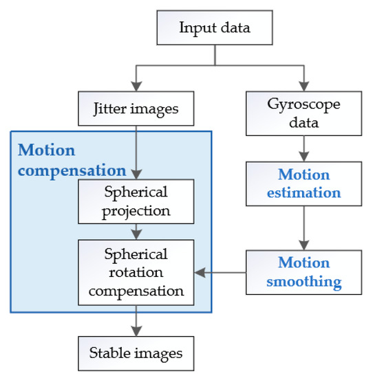
Figure 1.
Framework of the proposed algorithm.
Input data: when a jitter video is obtained, the gyroscope data are collected at the same time.
Motion estimation: the 3D rotation transformation of the camera attitude at an adjacent time is calculated by the gyroscope data, and the camera rotation path is obtained cumulatively.
Motion smoothing: the camera rotation path smoothing is transformed into a constrained regression problem on a Riemannian manifold, and the optimal solution is calculated to obtain a smooth rotation path.
Motion compensation: the image is projected on a spherical surface, and the jitter rotation component is compensated by rotating the spherical surface. Then, the image is projected inversely onto a plane to obtain a stable video.
3. Methodology
The proposed self-calibration spherical video stabilization based on a gyroscope includes three main steps: motion estimation, motion smoothing, and motion compensation.
3.1. Motion Estimation and Smoothing
In the 3D rotation estimation module, the gyroscope data are used to estimate the 3D rotation of the camera. The rotation angular velocity of a camera in the 3D coordinate system is obtained by the gyroscope, and the rotation angle is calculated with the integral of rotation angular velocity with respect to time, where is the sampling time interval of the gyroscope. Subsequently, the inter frame rotation matrix corresponding to the rotation angle can be obtained by Equation (1):
The camera path is represented by Equation (2):
where is the rotation matrix between ith frame and (i + 1)th frame.
All of rotation matrices constitute the special orthogonal group, where any element satisfies the constraint , which can be also considered as an embedded Riemannian submanifold. The metric of Riemannian manifold is geodesic distance as shown in Equation (3):
where is the matrix logarithm operator and is the Frobenius norm of a matrix.
The motion smoothing can be formulated as the objective function, and the smoothed trajectory is obtained by solving the following minimum optimization problem, as shown in Equation (4):
where is the smoothed trajectory, is the original trajectory, and is the weight controlling the smoothness of the stabilized trajectory. For each video sequence, the camera’s rotation in the 3D space can be mapped to a curve on a Riemannian manifold. The stable camera’s 3D rotation can be obtained by optimizing the geodesic distance of the curve in this space. As shown in Figure 2, the rotation matrix is transformed into a Euler angle to describe the original path and smooth the path using Equation (5):
where is the element of th row and th column in the rotation matrix .
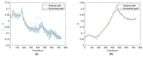
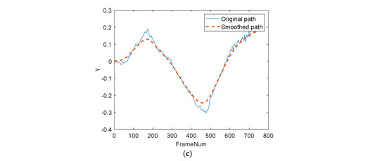
Figure 2.
Gyroscope path smoothing: (a) path smoothing; (b) path smoothing; (c) path smoothing.
The solid line is the original path, and the dotted line is the smoothed path. The smoothed path suppresses the jitter and retains the intentional motion.
3.2. Motion Compensation
Motion compensation is an important operation of video stabilization. The virtual sphere is first established by taking the optical center of the camera as the sphere center, and then each frame image is projected on a virtual spherical surface [16]. Next, the component causing the camera jitter will be obtained according to the difference between the smoothed camera path and the original path. Finally, the motion compensation is carried out by reversely rotating the spherical surface to compensate the jittered images.
3.2.1. Spherical Projection
According to the pinhole camera model, a 2D image coordinate system can be converted into a 3D spherical coordinate system. In this paper, the angle-based spherical projection method is used, and the model is shown in Figure 3.
Figure 3.
Spherical projection model.
The resolution of the image collected by the camera is set as , where is the image width and is the image height. In the spherical model of the right-handed coordinate system, the origin is the optical center of the pinhole camera; the axis is the optical axis and passes through the central point of the image; is the radius of the sphere as shown in Figure 3, and it is plotted as a red line; the projection of point in the world coordinate system is denoted as p in the image coordinate system (marked as ), which is centered at ; the projection of point in the virtual sphere is denoted as , which can be represented by angular coordinates; is the angle between and the axis, and is the angle between and the axis. Thus, can be calculated by Equation (6):
where is the radius of the sphere and is the pixel coordinates of the image.
The spherical coordinates of point is calculated by Equation (7):
In this way, the points in the image plane are converted to the corresponding points in the 3D sphere, which realizes the conversion of 2D plane images to 3D sphere images. As shown in Figure 4, taking the data published by Jia [12] as an example, the camera’s focal length of was used as the radius for spherical projection. Figure 4a is a 2D plan, and Figure 4b is the corresponding spherical projection.
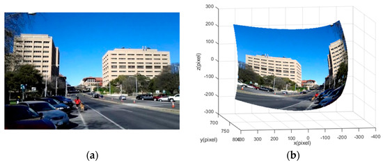
Figure 4.
Example of spherical projection: (a) two-dimensional (2D) image; (b) spherical projection image.
3.2.2. Self-Calibration of the Spherical Radius
As shown in Figure 5, the projected points of point on two adjacent frames and are and , respectively. The relative position deviation of and in two frames can be regarded as a jitter component. and are the angles between the corresponding spherical projected point and the optical axis. The rotation angle of relative to is denoted by , which conforms to the spherical rotation model with radius . Since the gyroscope is bound to the camera, can be obtained from the gyroscope data. The most important part is how to implement the spherical radius value , which determines the stabilization effectiveness. Take an example in Figure 5. When the radius of the sphere , the rotation angle is not equal to the rotation angle obtained by the gyroscope, which does not conform to the rotation mode of the gyroscope; when the radius of the sphere is , the rotation angle is equal to the rotation angle obtained by the gyroscope, which conforms to the imaging model of the camera and the rotation mode of the gyroscope.
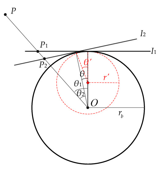
Figure 5.
Camera rotation model.
Therefore, it is necessary to calibrate spherical radius in accordance with the gyroscope rotation. The spherical radius should be the focal length of the camera in theory. To achieve the self-calibration of the spherical radius coupled with a different spherical radius , mean square error (MSE), which is used in image processing to measure the difference between two images, is used to filter the optimal spherical radius value. The MSE of a stable video corresponding with different spherical radius values is defined as Equation (8):
where is the number of the total frames in the video, and is the stable frame that is stabilized with radius . Thus, the optimal spherical radius is transformed into solving the optimization problem of Equation (8).
3.2.3. Spherical Rotation Compensation
The existing motion compensation methods transform a 3D rotation transformation relationship into a 2D image coordinate transformation relationship through the camera intrinsic parameter matrix [13]. Assuming that the camera intrinsic matrix is , which contains five intrinsic parameters, and represent focal lengths in terms of pixel, represents the skew coefficient between the axis and the axis, and cx and represent the principal points, which can be written as:
The pixel in any stable frame can be calculated by the following equation under pure 3D camera rotation:
where is the smoothed rotation matrix, is the original rotation matrix, , and are pixel points in the original image. The existing motion compensation methods depend on the intrinsic parameter matrix.
Different from the existing methods, the proposed method does not need the camera intrinsic parameter matrix to realize the video stabilization. The method proposed in this paper projects an image to a sphere and uses a rotation matrix to rotate the sphere for compensating the image. Owing to this, the rotation component causing jitter can be calculated based on the difference between the smoothed rotation matrix path and the original rotation matrix path. A relatively stable spherical image can be obtained using a rotation component to reversely rotate the spherical surface, as shown in Equation (10):
where is the original spherical point, is the spherical point after rotation, and is the rotation jitter component. Finally, the stable image sequence can be obtained by expanding the spherical surface. In Figure 6, taking the target point of th frame and ( + 1)th frame as the reference frame, point is dislocated between these two adjacent frames. In the third sphere, the spherical image of ( + 1)th frame is rotated to make its position relatively consistent, so as to achieve the effect of image stabilization.
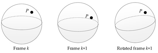
Figure 6.
Spherical rotation compensation model.
4. Experiment and Result Analysis
In this section, two groups of experiments are illustrated. The first experiment compared different spherical radius values to prove the optimality of the proposed self-calibration method, and the second experiment compared different motion compensation methods to demonstrate the effectiveness of the proposed spherical motion compensation method.
4.1. Experiment Setting and Videos
In order to verify the effectiveness of the proposed method, vs2015 was used to program on a PC (Inter core i5-8500 CPU, 3.00GHz, 8GB RAM). To test the general applicability of the proposal, we collected the experimental data from different cameras, which were bound with a gyroscope. The joint calibration of the camera and the gyroscope proposed by Fang Ming [17] was used to align the image with the gyroscope data.
To evaluate the video stabilization effect quantitively, the peak signal-to-noise ratio (PSNR), the structural similarity index (SSIM) [18], the cropping ratio, the distortion score, and the stability score [19] were used. The PSNR and the SSIM are the commonly used metrics in image processing to evaluate the degree of registration between image sequences. The principle of the PSNR is that if the relative change between two adjacent frames is fully compensated, the pixel difference of two stable frames should be zero. The SSIM is widely used in video stability estimation. It considers brightness, contrast, and structure information to measure the similarity of two given images. The larger the PSNR value and the closer the SSIM value are to 1, the better the image stabilization effect is [18]. The computation methods of the PSNR and the SSIM are defined in Equation (11):
where and Ik+1 are the gray images of two adjacent frames; and are the gray averages of and , respectively; and are the gray variances of and , respectively; is the gray covariance of and ; , , , , and are the constants used to maintain stability.
The cropping ratio measures the remaining after cropping away empty regions. The distortion score is estimated from the affine part of homography. The stability score measures the smoothness of stabilized videos [19].
4.2. Comparison of Different Spherical Radius Values
In order to verify the effectiveness of spherical radius self-calibration, two groups of experimental data were implemented: (1) public video data and gyroscope data; (2) the video collected from the cascaded camera and gyroscope.
Firstly, public video data and gyroscope data [12] were used, and the focal length of the camera was pixels. The optimal spherical radius value was located at pixels, which was calibrated by the proposed method in Section 3.2.2. The deviation between the computed value and the focal length value was small and acceptable, since the centers of the gyroscope and the camera could not completely coincide and the computed value also conformed to the imaging model basically. We ranged the spherical radius values from 200 to 3000 pixels. The PSNR and SSIM values of different spherical radius values are shown in Figure 7. The optimal values were obtained at pixels, which indicated that the calibration result of the spherical radius is reliable. In addition, the larger the distance from the optimal radius was, the worse the video stabilization effect was.
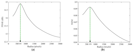
Figure 7.
Stability assessment of different spherical radii: (a) peak signal-to-noise ratio (PSNR) stability assessment; (b) structural similarity index (SSIM) stability assessment.
Secondly, the video data were collected from the cascaded camera and gyroscope, where the image data and gyroscope data were registered. The relationship between the camera and the gyroscope is shown in Figure 8. The focal length of pixels was computed through the camera calibration. The spherical radius value obtained by the proposed self-calibration method was pixels. Three groups of data, including video data and gyroscope data, were collected to verify the validity of the calibration results. We ranged the spherical radius values from 200 to 3000 pixels. Figure 9 exhibits the PSNR and SSIM values of the three videos corresponding to different spherical radii, respectively. It can be found that the PSNR values of the three videos are the maximum at and the SSIM values closest to 1 are at , which indicates that the calibration result of the spherical radius is reliable.
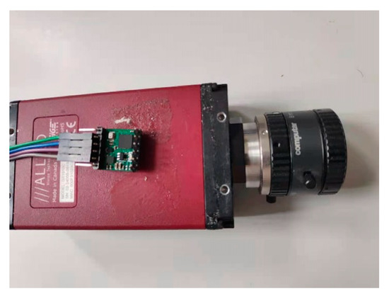
Figure 8.
The relationship between the camera and the gyroscope.
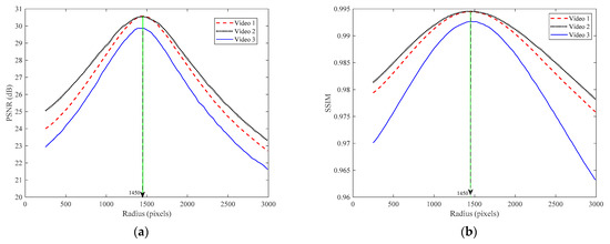
Figure 9.
Assessment of video stabilization results with different spherical radii: (a) comparison of PSNRs; (b) comparison of SSIMs.
Therefore, the optimal spherical radius was basically consistent with the focal length of the camera, and the results obtained by the proposed self-calibration method conformed to the rotation model of the camera.
4.3. Comparison with the Intrinsic Parameter Matrix Method
In this paper, three different camera data were used to compare the image stabilization effect of spherical motion compensation and intrinsic parameter matrix compensation methods [12,13,15]. Figure 10 is a thumbnail of three videos, where video 1 is an indoor scene, video 2 is an outdoor scene, and video 3 is a feature-deficient scene. All the resolutions of the three videos were 1280 pixels × 720 pixels. We used the PSNR, the SSIM, the cropping ratio, the distortion score, and the stability score to compare the video stabilization effect. The results of these methods are shown in Table 1, Table 2 and Table 3. It can be seen that the proposed method achieves better indices. Meanwhile, we compared runtime as shown in Table 4. The runtime of the proposed method is slower than those of the methods [13,15], but it is promising to achieve real-time processing under the best stabilization effect. Moreover, the proposed method does not need to calibrate in advance.
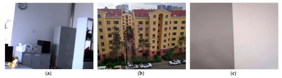
Figure 10.
Video thumbnail: (a) video 1; (b) video 2; (c) video 3.

Table 1.
Video stabilization effect comparison of video 1.
Table 2.
Video stabilization effect comparison of video 2.
Table 3.
Video stabilization effect comparison of video 3.
Table 4.
Single-frame time consumptions of different video stabilization methods.
4.4. Discussion
The proposed stabilization method uses a gyroscope to suppress random jitter effectively by a self-calibration spherical compensation model. At present, the representative classical methods of video stabilization based on a gyroscope include research [12,13,14,15]. We have carried out comparative analysis with references [12,13,15], which demonstrates that the proposed method has advantages in video stabilization effect and convenience. The method described in [14] designs a special optical flow sensor to assist video stabilization. There are no public sensor data and video data, so it is difficult for us to compare the results reported in this paper with those in [14].
In addition, the characteristic of this method is that it can avoid extra calibration work. In practical applications, in any scene, the image can be stabilized by fixing a gyroscope on a camera, which is more flexible and ensures the video stabilization effect. However, the runtime of the proposed method is not the fastest compared with those of other methods, but it is promising to achieve real-time processing under the best stabilization effect. In the next stage, we will optimize the method to reduce runtime.
5. Conclusions
In this paper, a self-calibration spherical compensation image stabilization method based on a gyroscope has been proposed. The camera motion trajectory is obtained by gyroscope, and its trajectory is smoothed on a Riemannian manifold to obtain a jitter component; the virtual sphere is established by the optical center of the camera, and the objective function about the spherical radius is established according to the mean square error of the stabilized video. The optimal spherical radius is determined by solving the optimal value of the objective function to complete the spherical radius calibration. Then, the image is projected on the spherical surface, and the spherical surface is rotated reversely according to the jitter component for motion compensation. Finally, the spherical image is expanded to obtain a stable video sequence. The experimental results showed that the stability metrics, i.e., the PSNR, the SSIM, the cropping ratio, the distortion score, and the stability score, were improved, demonstrating that the proposed method is better than the traditional intrinsic parameter matrix compensation methods. Moreover, the proposed stabilization method not only maintains the effectiveness of video stabilization, but also relaxes the dependence on camera calibration.
Author Contributions
All three authors contributed to this work. Methodology, Z.R. and M.F.; writing—original draft preparation, Z.R.; writing—review and editing, M.F. and C.C.; supervision, C.C.; project administration, M.F.; funding acquisition, M.F. and C.C. All authors have read and agreed to the published version of the manuscript.
Funding
This research was funded by the National Natural Science Foundation of China (grant number: U19A2063) and the Jilin Provincial Science & Technology Development Program of China (grant numbers: 20190302113GX and 20170307002GX).
Data Availability Statement
The data used to support this study’s findings are available from the author upon request.
Conflicts of Interest
The authors declare no conflict of interest.
References
- Zhao, M.D.; Ling, Q. Adaptively Meshed Video Stabilization. IEEE Trans. Circuits Syst. Video Technol. 2020, 1. [Google Scholar] [CrossRef]
- Wu, R.; Xu, Z.; Zhang, J.; Zhang, L. Robust Global Motion Estimation for Video Stabilization Based on Improved K-Means Clustering and Superpixel. Sensors 2021, 21, 2505. [Google Scholar] [CrossRef] [PubMed]
- Akira, H.; Katsuhiro, H. Sensorless Attitude Estimation of Three-degree-of-freedom Actuator for Image Stabilization. Int. J. Appl. Electromagn. Mech. 2021, 6, 249–263. [Google Scholar]
- Shankarpure, M.R.; Abin, D. Video stabilization by mobile sensor fusion. J. Crit. Rev. 2020, 7, 1012–1018. [Google Scholar]
- Raj, R.; Rajiv, P.; Kumar, P.; Khari, M.; Verdú, E.; Crespo, R.G.; Manogaran, G. Feature based video stabilization based on boosted HAAR Cascade and representative point matching algorithm. Image Vis. Comput. 2020, 2020, 103957. [Google Scholar] [CrossRef]
- Hu, X.; Olesen, D.; Knudsen, P. Gyroscope Aided Video Stabilization Using Nonlinear Regression on Special Orthogonal Group. In Proceedings of the 2020 IEEE International Conference on Acoustics, Speech and Signal Processing (ICASSP), Barcelona, Spain, 4–8 May 2020; pp. 2707–2711. [Google Scholar]
- Wang, Z.M.; Xu, Z.G. A Survey on Electronic Image Stabilization. J. Image Graph. 2010, 15, 470–480. [Google Scholar]
- Huang, W.Q.; Dang, B.N.; Wang, Y.; Sun, M.X. Two-freedom image stabilization institution of large stroke of bidirectional actuation. Opt. Precis. Eng. 2017, 25, 1494–1501. [Google Scholar] [CrossRef]
- Rodriguez-Padilla, I.; Castelle, B.; Marieu, V.; Morichon, D. A Simple and Efficient Image Stabilization Method for Coastal Monitoring Video Systems. Remote Sens. 2020, 12, 70. [Google Scholar] [CrossRef] [Green Version]
- Guilluy, W.; Oudre, L.; Beghdadi, A. Video stabilization: Overview, challenges and perspectives. Signal Process. Image Commun. 2021, 2021, 116015. [Google Scholar] [CrossRef]
- Cao, M.; Zheng, L.; Jia, W.; Liu, X. Real-time video stabilization via camera path correction and its applications to augmented reality on edge devices. Comput. Commun. 2020, 158, 104–115. [Google Scholar] [CrossRef]
- Jia, C.; Evans, B.L. Constrained 3D Rotation Smoothing via Global Manifold Regression for Video Stabilization. IEEE Trans. Signal Process. 2014, 64, 3293–3304. [Google Scholar] [CrossRef]
- Yang, J.; Lai, L.; Zhang, L.; Huang, H. Online Video Stabilization Algorithm on Lie Group Manifold. Pattern Recognit. Artif. Intell. 2019, 32, 295–305. [Google Scholar]
- Pengwei, Z.; Yuanji, J.; Chao, D.; Tian, L.; Shichuan, H. Video Stabilization Technique Based on Optical Flow Sensor. Opto-Electron. Eng. 2019, 46, 180581. [Google Scholar]
- Zhuang, B.; Bai, D.; Lee, J. 5D Video Stabilization through Sensor Vision Fusion. In Proceedings of the 2019 IEEE International Conference on Image Processing, Taipei, Taiwan, 22–25 September 2019; pp. 4340–4344. [Google Scholar]
- Ren, Z.W.; Fang, M.; Chen, C.Y.; Kaneko, S.I. Video stabilization algorithm based on virtual sphere model. Electron. Imaging 2021, 30, 1–18. [Google Scholar] [CrossRef]
- Fang, M.; Tian, Y. Robust Electronic Image Stabilization Method Based on IMU-Camera Calibration. Inf. Control 2018, 47, 156–165. [Google Scholar]
- Chen, B.H.; Kopylov, A.; Huang, S.C.; Seredin, O.; Karpov, R.; Kuo, S.Y.; Lai, K.R.; Tan, T.-H.; Gochoo, M.; Hung, P.C.K. Improved global motion estimation via motion vector clustering for video stabilization. Eng. Appl. Artif. Intell. 2016, 54, 39–48. [Google Scholar] [CrossRef]
- Zhao, M.D.; Ling, Q. PWStableNet: Learning pixel-wise warping maps for video stabilization. IEEE Trans. Image Process. 2020, 2020, 3582–3595. [Google Scholar] [CrossRef] [PubMed]
Publisher’s Note: MDPI stays neutral with regard to jurisdictional claims in published maps and institutional affiliations. |
© 2021 by the authors. Licensee MDPI, Basel, Switzerland. This article is an open access article distributed under the terms and conditions of the Creative Commons Attribution (CC BY) license (https://creativecommons.org/licenses/by/4.0/).