Article

Resource Recommender for Cloud-Edge Engineering

by
Amirmohammad Pasdar
1,
Young Choon Lee
1,*,
Tahereh Hassanzadeh
2 and
Khaled Almi’ani
3,4
1
Department of Computing, Macquarie University, Sydney 2109, Australia
2
School of Engineering and Information Technology, University of New South Wales, Canberra 2610, Australia
3
Higher Colleges of Technology, Fujairah, United Arab Emirates
4
Department of Computer Science, Al-Hussein Bin Talal University, Ma’an 71111, Jordan
*
Author to whom correspondence should be addressed.
Information 2021, 12(6), 224; https://doi.org/10.3390/info12060224
Submission received: 1 May 2021 / Revised: 18 May 2021 / Accepted: 20 May 2021 / Published: 25 May 2021
(This article belongs to the Special Issue Smart Cyberphysical Systems and Cloud–Edge Engineering)

Abstract

:
The interaction between artificial intelligence (AI), edge, and cloud is a fast-evolving realm in which pushing computation close to the data sources is increasingly adopted. Captured data may be processed locally (i.e., on the edge) or remotely in the clouds where abundant resources are available. While many emerging applications are processed in situ due primarily to their data intensiveness and short-latency requirement, the capacity of edge resources remains limited. As a result, the collaborative use of edge and cloud resources is of great practical importance. Such collaborative use should take into account data privacy, high latency and high bandwidth consumption, and the cost of cloud usage. In this paper, we address the problem of resource allocation for data processing jobs in the edge-cloud environment to optimize cost efficiency. To this end, we develop Cost Efficient Cloud Bursting Scheduler and Recommender (CECBS-R) as an AI-assisted resource allocation framework. In particular, CECBS-R incorporates machine learning techniques such as multi-layer perceptron (MLP) and long short-term memory (LSTM) neural networks. In addition to preserving privacy due to employing edge resources, the edge utility cost plus public cloud billing cycles are adopted for scheduling, and jobs are profiled in the cloud-edge environment to facilitate scheduling through resource recommendations. These recommendations are outputted by the MLP neural network and LSTM for runtime estimation and resource recommendation, respectively. CECBS-R is trained with the scheduling outputs of Facebook and grid workload traces. The experimental results based on unseen workloads show that CECBS-R recommendations achieve a ∼65% cost saving in comparison to an online cost-efficient scheduler (BOS), resource management service (RMS), and an adaptive scheduling algorithm with QoS satisfaction (AsQ).

1. Introduction

Cost efficiency has been a major driving force for the wide adoption of public clouds, such as Amazon Web Services (AWS) [1], Microsoft Azure (MS) [2], Google Cloud Platform (GCE) [3], and Alibaba Cloud (AC) [4], particularly with the pay-as-you-go pricing. These clouds host servers distributed around the world to provide nearly every Information and Communications Technology (ICT) service (e.g., emails, social media, e-commerce and e-health). While cloud resources are in the core network, pushing computing close to the data sources (i.e., resources residing at the network’s edge) is extensively being adopted for the low latency and privacy preserving scheduling of data processing jobs. Scheduling can be further motivated by considering the role of artificial intelligence (AI) in recommending cost-efficient resources in the edge-cloud environment.
There have been many studies, with public clouds and edge-cloud environments (i.e., hybrid clouds), e.g., [5,6,7,8,9,10,11,12], aimed at minimizing resource usage, resulting in cost reduction with the consideration of some constraints, such as deadline and monetary budget. However, these studies tend to overlook privacy and the utility/energy cost of edge resources. Besides, their performance goals are often achieved with an assumption of prior knowledge of job characteristics (runtimes in particular) [13,14].
While the availability of accurate job information is largely unrealistic, the estimation of such information with reasonable accuracy is possible with the help of recent advances in machine learning. In particular, the recent Microsoft Azure traces [15,16] show that workloads/jobs arriving at a particular cloud often have similar characteristics and resource requirements. Therefore, learning such information through machine learning techniques [17,18] can facilitate edge-cloud scheduling and can be beneficial, not only for runtime estimation, but also for resource recommendations. Hence, we address the problem of cost-efficient job scheduling in an edge-cloud environment while preserving privacy through recommendations. The scheduling not only considers public cloud billing cycles and the edge utility cost, but also relies on runtime estimations for resource recommendation. As an extensive extension to our previous work [19], the CECBS-R framework is assisted by machine learning techniques to facilitate scheduling through runtime estimations and recommendations, as well as improving edge resource utilization while reducing energy consumption.
To this end, we propose Cost Efficient Cloud Bursting Scheduler and Recommender (CECBS-R) framework that is assisted by ANNs, i.e., RNN (recurrent neural network) and LSTM, to deal with scheduling and recommendation while preserving privacy. Figure 1 shows the overall CECBS-R structure. CECBS-R consists of a cloud state controller (CSC) (Algorithm 1) and a cloud scheduler (CS) (Algorithm 2). The Cloud State Controller periodically collects information about jobs in the edge-cloud environment and the edge resource utilization to be processed by ANNs for recommendations. Edge resources (e.g., servers) are constantly monitored, and based on the recommendations, they may become activated or deactivated. The Cloud Scheduler considers feasible recommendations for scheduling jobs through a particle swarm-based algorithm, taking into account the workload’s objectives and constraints. Moreover, the MLP neural network employed in the CECBS-R profiles jobs and assists runtime estimation through the collected information in the edge-cloud environment.
CECBS-R has been evaluated in two phases, based on Facebook workload traces (including synthesized traces), grid workloads [20,21], and the real-world resource requirement traces [15]. The first phase evaluates the cost efficiency of CECBS-R scheduler in comparison to an adaptive scheduling algorithm with QoS satisfaction (AsQ) [22], online cost-efficient scheduler (BOS) [6], and resource management service (RMS) [5]. In the second phase, CECBS-R is trained by the executed workload information of the previous phase to schedule new workload traces based on the recommendation results. The experimental results show that CECBS-R scheduler on average achieves ∼67% cost-saving in comparison to BOS, RMS, and AsQ. Moreover, recommendations produced by ANNs for a set of new workloads achieved a ∼65% cost saving.
The remainder of the paper is organized as follows. In Section 2, the model and problem statement are defined, followed by Section 3, which explains CECBS-R in detail. Results are discussed in Section 4. We review the related work in Section 5 and conclude this paper in Section 6.

2. Models and Problem Formulation

In this section, the application and system models are described, and the problem is formulated. The symbols used in this paper are described in Table 1.

2.1. The Multi-Cloud

The multi-cloud environment ( M C ) in this study comprises an edge (R) and P public cloud providers ( C P ), each of which has a set of resources ( R C P ).
M C = R + 1 p R C P

2.1.1. Public Clouds

Resources in public clouds are virtually unlimited, and they are virtualized and called virtual machines (VMs). Each virtual machine ( v m i ) is recognized by its computation capacity in terms of vCPUs and memory, storage space, and available bandwidth. Each public cloud ( C P i ) maintains a specific billing cycle ( B C i ) to determine user resource consumption. Moreover, there is an approximate VM deployment time for each C P i to have VMs ready.
When a user launches a VM, an active cycle ( B C i a ) becomes available and can be used for free within the active period. Otherwise, a new cycle ( B C i n ) is created that will incur charges. Moreover, each public cloud provider ( C P i ) may possess unused resource capacities known as preemptible VMs [3,4], spot instances [1], or low priority VMs [2]. These resources may be offered at a cheaper price and/or based on a specific duration (up to six hours for spot instances [1] or an hour for Alibaba Cloud [4]). Also, each public cloud provider ( C P i ) may come with an interruption (i.e., decommissioning) probability for unused resources. This probability describes how often resources may be decommissioned [1].
Moreover, a cloud provider ( C P i ) charges users whenever VMs consume storage and bandwidth determined in GigaBytes (GB) during a period. In other words, if a cloud provider ( C P i ) charges B i per b consumed bandwidth and S i per s consumed storage for duration d s , the expected cost ( E C i ) is defined as follows.
E C i = B i × b + S i × s × d s
To compute the cost of public clouds, we define E C C P in Equation (3) as the summation of all active billing cycles for each public cloud provider ( | B C i | ) and the cost of consumed storage and bandwidth.
E C C P = i = 1 P , | B C i | B C i a + i = 1 P E C i

2.1.2. The Edge

The edge is a cluster of resources (R) where it has a fixed number of homogeneous servers (m), each of which has storage capacity, a certain number of CPU cores ( m i c o r e ), and available memory ( m i m e m ). Each server ( m i ) within the cluster consumes electricity for operating that is measured in watts ( ω ). Electricity may have volatile charging rates ( ω v ) at different times of the day or may follow fixed rates ( ω f ) per kilowatt-hour ( k ω -h).
Servers may have different utilization rates ( U T i ) during workload execution that require a wattage usage (i.e., energy supply) based on the hardware specifications [23]. Hence, the cluster may be controlled by adding ( m i ) or removing servers ( m i ) for energy consumption management. Equation (4) computes the expected wattage usage per server utilization ( U T i ). Each server utilization ( U T i ) is bound between a lower utilization ( U T L B ) and upper utilization ( U T U B ) which ties the wattage usage to their lower-bound ( ω U T L B ) and upper-bound ( ω U T U B ) wattage usage, respectively.
ω i = U T i U T L B U T U B U T L B × ( ω U T U B ω U T L B ) + ω U T L B
However, Equation (4) presents a linear energy consumption model in comparison to non-linear models in the literature (e.g., [24,25]), Fan et al. [26] showed with empirical results that the linear model could reasonably estimate power consumption.
Hence, if there are k active servers inside the edge, the total edge energy cost ( E C ω ) per volatile (or fixed) electricity rates for the period τ are expressed as follows.
E C ω = i = 1 k , τ ω i × ω v
Considering the edge electricity cost, the total edge-cloud cost is stated as follows.
E C M C = E C ω + E C C P

2.2. Workloads

Workloads are defined as a stream of jobs (T) which become available at time τ at the edge. Each job ( t i ) is recognized based on the characteristics it maintains. These characteristics are defined as the job resource requirements ( R i t ), submission time ( t i τ ), deadline ( D i t ), privacy status, recommended cloud environment ( R C i t ), and estimated runtime ( E R T i t ). R i t is also expressed as number of CPU cores ( R i t c o r e ), required memory ( R i t m e m ) and storage ( R i t s ).
Each job ( t i ) also belongs to a category that correlates D i t to the category’s characteristic defined as interactive or delay-insensitive [15]. Moreover, jobs in a workload are categorized into three job classes referred to as small, medium, and long-running jobs [15,27].
When a server/VM finishes a job ( t i ), the job has an actual runtime ( A R T i t ) that is recorded for the runtime estimation of future jobs alongside the job(s) resource requirements. This job ( t i ) may be assigned to a feasible cloud recommendation ( R C i t ) and may maintain an estimated cost with respect to either A R T i t or an estimated runtime ( E R T i t ).
The estimated runtime belongs to a coarse-grained classification with respect to the per-hour billing policy up to 24 h of a day in the form of a one-hot vector. Moreover, there is a controller ( γ i ) for a job ( t i ) that illustrates the runtime duration within 24 h. This is due to the fact that, if a job may run for a day, it is very likely to run longer [15], thus, although in the literature the runtime may be assumed available, in reality, it is not trivial to estimate the runtime of jobs running for more than a day. Hence, γ i is defined as follows.
( γ i , t i ) = 0 A R T i t 24 1 O t h e r w i s e .

2.2.1. Workload Execution Location

In the absence of the recommended cloud/edge for a job, the execution location heuristically relies on the expected execution cost of a job ( E C i t ). This cost is computed based on the job runtime (e.g., E R T i t ), but it is not always available.
When a job runtime is not available, the estimated cost per specified coarse-grained duration (d) in the edge-cloud environment is computed. The duration is categorized into four time-period classes which are referred to as 1-h [1,2,3,4] and 6-h [1], which represent billing cycles of public clouds, 12-h, and 24-h duration. The 12-h and 24-h are considered due to the volatile electricity rates applied to the utility cost in the edge.
Since the billing cycle cost for the specified duration does not change, it is necessary to estimate the runtime cost in the edge. In other words, how much the cost would be if a job fell into the consecutive rate types that are shown in Figure 2. The consecutive rate would be (1) off-peak → shoulder, (2) shoulder → peak → shoulder, or (3) peak → shoulder → off-peak for 12-h runtime duration. The 24-h duration would fall into any combination of the off-peak, shoulder, and peak rates, and it would take into account all the rates for the cost estimation (see Figure 2).
( R C i t , E C i t ) = min i d min j B C E C C P , i d E C ω
When the runtime is not available, Equation (8) returns the minimum cost, which is proven by contradiction in Lemma 1.
Lemma 1.
Given two numbers α and β to represent the edge and public clouds cost computed by Equation (8), respectively, there is a real number c such that c = min ( α , β ) .
Proof. 
It is assumed that there is a c ; c < c and it can be written as c = min ( α , β ) in which α and β are the new minimums.
If β < β , public cloud billing cycles have volatile rates per specific duration which are against the fact that the rate is fixed, hence, β = β .
Job t i becomes available at t i τ and suppose α < α which is computed based on four time-period classes; d j { d 1 , d 6 , d 12 , d 24 } . We replace α < α considering the job arrival time to compute the expected cost by Equation (5) for each time period.
t i τ + { d 1 , d 6 , d 12 , d 24 } < t i τ + { d 1 , d 6 , d 12 , d 24 }
Since the electricity rate for the off-peak, shoulder, and peak are not volatile, the expected cost for α and α is identical, which means α = α , thus, c = c .  □
When the job runtime (i.e., the estimated runtime ( E R T i t )) is provided, the expected cost is computed either based on the recommended cloud environment ( R C i t ) or through a cost comparison with respect to E R T i t for choosing a cloud/edge environment with minimum cost.
( R C i t , E C i t ) = min ( E C C P , E C ω ) R C i t = E C R C i t O t h e r w i s e .

2.3. Problem Statement

CECBS-R for a given stream of tasks T aims to reduce scheduling execution cost while maintaining quality of service (QoS) in the edge-cloud environment.
min t T E C M C
The scheduling has to take into account the runtime uncertainties which is assisted with ANNs’ recommendations. In other words, the problem in our study is two folds. Firstly, how to schedule workloads within the edge-cloud environment when runtime uncertainties exist while preserving privacy in a cost-efficient manner. Secondly, how scheduling can be facilitated with recommendations made by ANNs in the edge-cloud environment.

3. Cost Efficient Cloud Bursting Scheduler and Recommender (CECBS-R)

This section details CECBS-R (Figure 1) components; cloud state controller (Algorithm 1) and cloud scheduler (Algorithm 2), which are assisted with ANNs.

3.1. Cloud State Controller

Cloud state controller leverages ANNs for runtime estimation, as well as recommendations to be used for server management in the edge and the job cloud/edge recommendation.
ANNs are computing systems in which examples (i.e., job information or server utilization) are learnt for performing operations, e.g., in terms of cloud environment recommendation or server management. Each neural network consists of connected neurons placed in network layers, and transformations are applied to the value of neurons. Transformations are done by non-linear activation functions to output a value for transmission to the next layer through the network edges. Thus, each value goes through consecutive network layers, starting from an input layer, one layer, or multiple hidden layers and terminating at the output layer. Neurons and edges in a neural network are assigned weights that are adjusted during the network training.
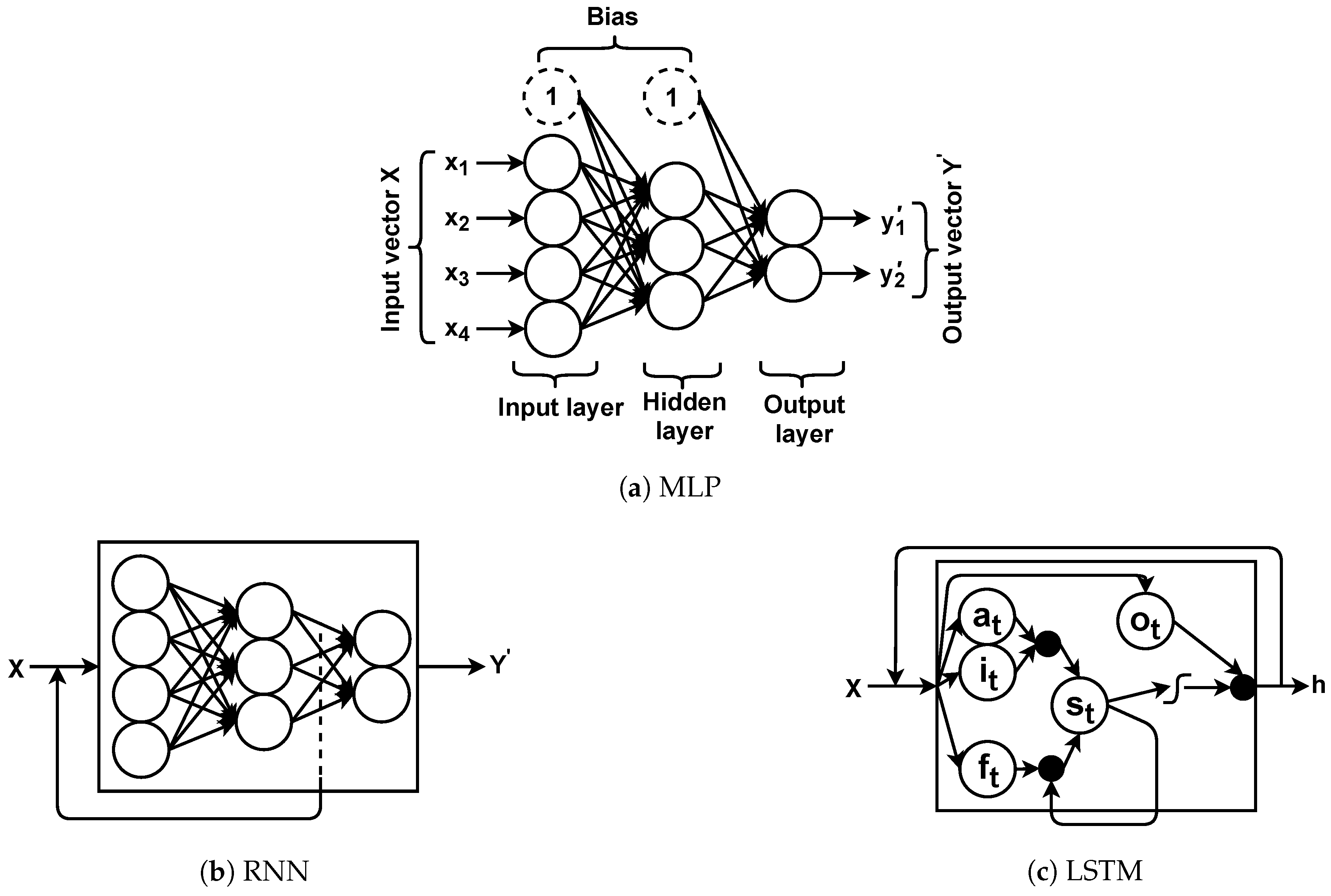
Neural networks used in this study are in different forms referred to as MLP, RNN, or LSTM [29], which are shown in Figure 3.
The MLP is a feed-forward neural network that is trained per each input vector in a supervised manner by backpropagation algorithm with respect to the actual outputs or labels (i.e., Y = [ y 1 , , y o ] ). The MLP repeats the process (e.g., classification) for new inputs, and weights are adjusted accordingly. RNN is a special form of MLP that any learnt (i.e., the hidden layer weights) information is kept and is passed to the next input. In fact, RNNs are a chain of MLPs that leverage shared weights for training. This is to ensure that any prediction/estimation is outputted based on the seen input information.
Although promising, during the learning process, less past/seen information contributes to the training (i.e., weight adjustments) and it is known as a vanishing gradient. This drawback is addressed by LSTMs as the special form of RNNs comprised of gates to control information flow in the learning process. They also have a chain structure consisting of cells, each of which has four gates; forget gate, input gate, input activation gate, and output gate. The information that should be ignored from a cell is dealt with by the forget gate ( f t ). To decide what information should be stored in the cell state, there are two gates called input ( i t ) and input activation ( a t ) gates that contribute to the cell state. Finally, it is required to decide what information should be outputted, which is handled by the output gate ( o t ).
A neural network receives an input vector (i.e., X = [ x 1 , , x i ] ) and outputs an estimated (or interchangeably predicted) output vector (i.e., Y = [ y 1 , , y o ] ) which can be written as Y = f ( X ) . Neurons in the neural network layers are assigned weights w j k l that contribute to the neuron output ( a j l ) and are interpreted as the weight from k th neuron in the ( l 1 ) th layer to the j th neuron in the l th layer. Moreover, there are extra neurons called bias that hold a value equal to 1 and are connected to the neurons for shifting the activation function output. Hence, a neuron output ( a j l ) based on sigmoid ( σ ) (or tangent hyperbolic ( t a n h ) or softmax) activation function is defined as follows.
a j l = σ ( k w j k l a k l 1 + b j l )
To adjust the neural network weights in ANNs, the actual output vector (Y) is compared with the predicted output ( Y ) to compute the error (or loss), e.g., mean squared error (MSE). It computes the difference between the N real outputs and the predicted outputs for weight adjustments calculated as follows.
E = k ( y k y k ) 2 2 × N = k ( a k L y k ) 2 2 × N
Without loss of generality, if the neural network weight is W, the weight adjustment with respect to the computed error (E) is defined as follows.
W = W γ W E
In Equation (13), is the vector differential operator and γ is the learning variable that controls the weight adjustment. The weight adjustment process takes place by the usage of the backpropagation algorithm that performs repetitive procedures in two separate phases; forward pass ( A N N F W ) and backward pass ( A N N B W ). In the former, the input data is fed into the network to produce the predicted results with respect to Equation (11). In the latter, the error is calculated in Equation (12) and is propagated back to the neural network to update the network weights.
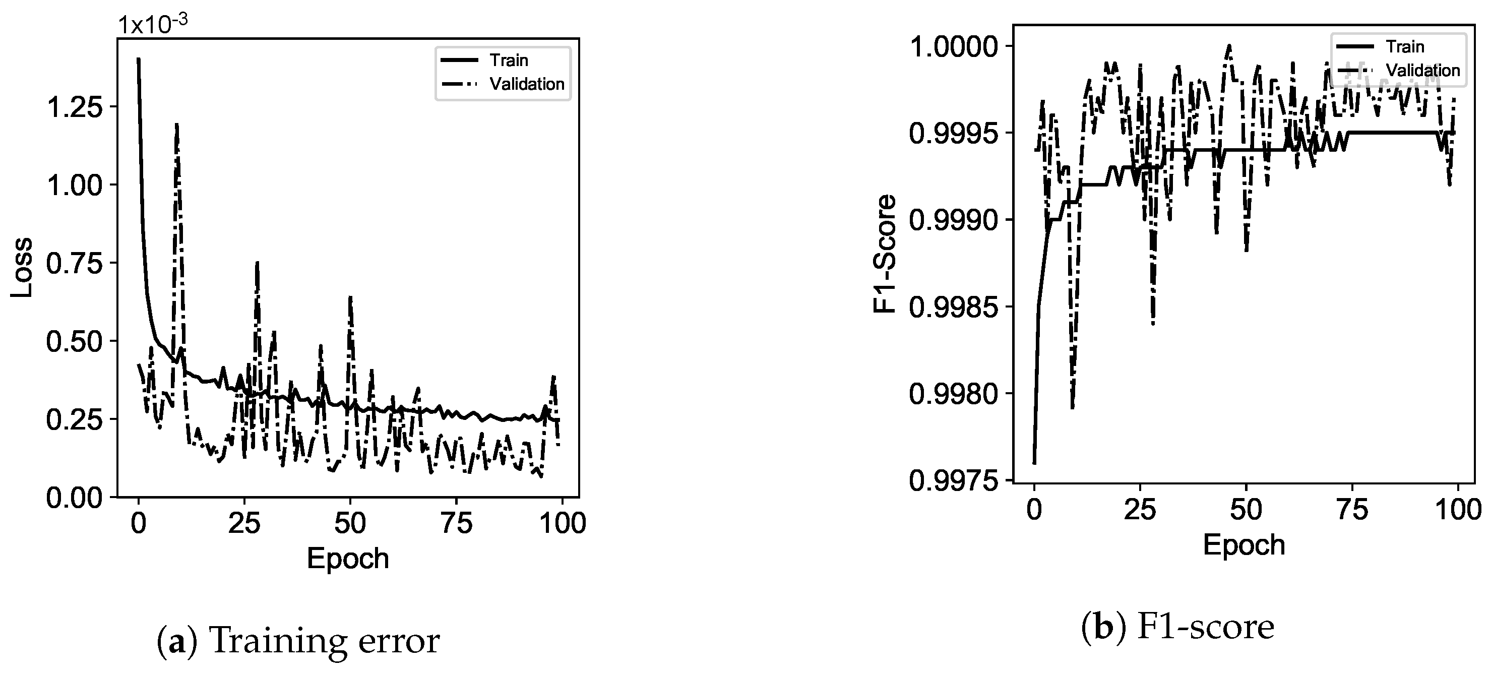
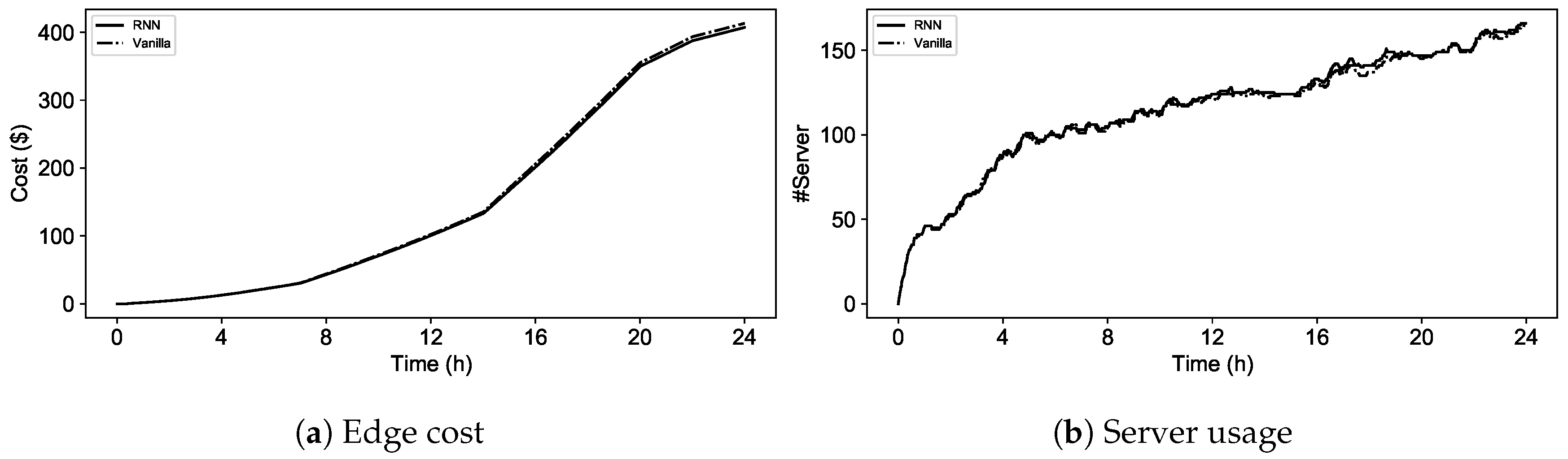
Considering the ANNs background stated in this section, the RNN is used to control server energy consumption in the edge by autonomously and periodically observing the server utilization. Servers within the edge may be deactivated or activated by a recommended signal. When the signal implies deactivation, a server puts it in deep sleep mode and is added to the idle server list ( I ). Otherwise, it activates a server from the idle list and is added to the active server list ( A ). Controlling active servers ( A ) for reducing energy consumption in the edge requires cluster utilization (i.e., CPU and memory) at and till time τ . This criterion fits in the RNN definition which considers that past seen information for recommendations. Therefore, the RNN is used for the edge server management per specific time intervals to send a signal for activation ( m i A ) or deactivation ( m i I ), in the case of putting servers in a deep sleep mode to reduce energy consumption.
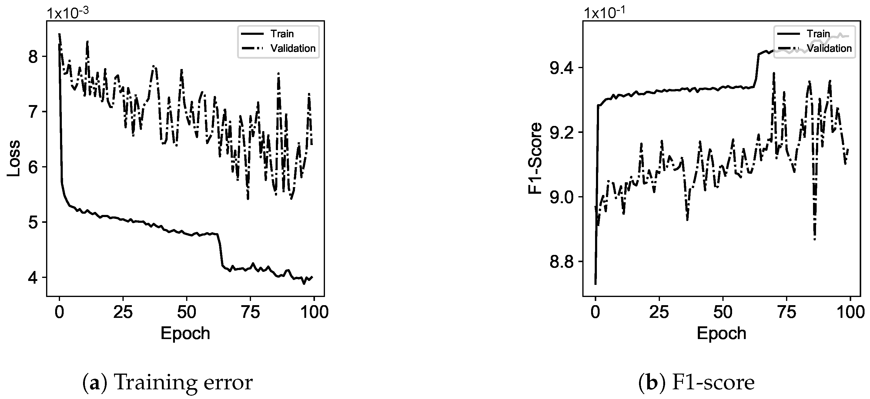
LSTM uses collected information of jobs in the edge-cloud environment for cloud/edge recommendations. The information is job characteristics and resource requirements that autonomously and per specified interval is logged due to the unknown job finish time. LSTM models univariate time series recommendation problems in which single series of observations exist (i.e., the job specifications including the executed edge/cloud environment) with respect to the past observations of jobs to recommend the next value in the sequence. Moreover, compared to the server management, additional information is available for cloud/edge recommendations that necessitates the usage of a sophisticated ANN (i.e., LSTM) for dealing with learning. Although RNN and LSTM rely on the historical context of input, LSTM provides a modulated output controlled by gates facilitating when to learn or forget, and mitigates the downsides of RNNs.
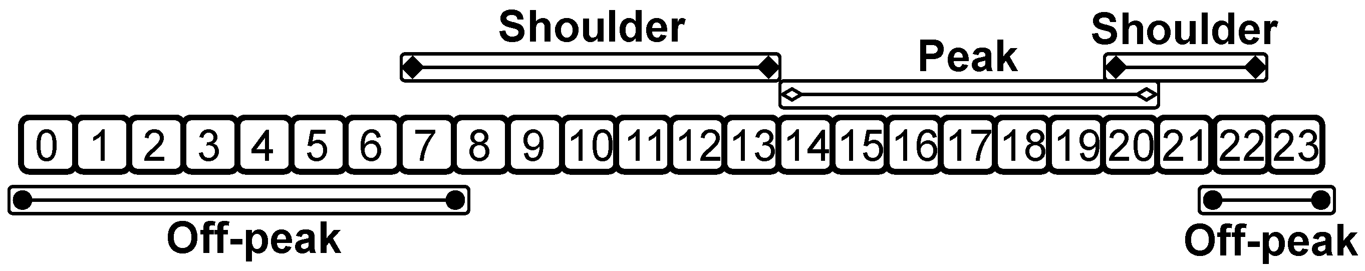
Finally, the job runtime estimation belongs to a coarse-grained classification problem, meaning that the runtime is classified into a time slot class (Section 2.2). Formally, for a job t j , the classification is interpreted as the time slot γ j with respect to Equation (7). This classification is controlled by the MLP neural network that uses the collected information about executed jobs across the edge-cloud environment, which are kept as profiles. Moreover, in the absence of a job runtime, the job cloud recommendations will not be reliable. This is due to runtime estimations to tailor the scheduling decision that uncertainty about the job runtime could blindly lead to an inefficient resource assignment and would affect the quality of scheduling and the cost [13,14].
Algorithm 1 presents an overview of the cloud state controller algorithm. This algorithm consists of procedures with respect to recommendation and runtime estimation, and they interact with the train procedure to obtain the corresponding weights for recommendation purposes.
The train procedure takes input datasets (i.e., the server utilization information and job specifications) and separately trains the corresponding ANN under a specified epoch (lines 1–11). The next procedure controls the edge servers with respect to the given utilization, followed by runtime estimation and recommendation procedures. The algorithm returns the estimated runtime, recommended cloud/edge, and active/idle edge server list.
Algorithm 1: Cloud State Controller (CSC).
Information 12 00224 i001

3.2. Cloud Scheduler

In this section, we explain how the Cloud Scheduler component (Algorithm 2), which was shown in Figure 1, deals with workload scheduling. The cloud scheduler is a dual-function algorithm that considers runtime estimations for scheduling and may follow recommendations for workload scheduling across the edge-cloud environment.
The cloud scheduler (Algorithm 2) relies on Equation (8) in the absence of cloud recommendations to heuristically examine which environment—the edge or public clouds—would be cost efficient for scheduling. This algorithm illustrates the workload scheduling across the edge-cloud environment which relies on a particle swarm optimization (PSO)-based algorithm for the edge. The algorithm takes into account runtime estimation or cloud/edge recommendations for scheduling decisions. Scheduling in the edge takes place when a job is privacy-sensitive or it is cost efficient to execute regular jobs with respect to active/idle servers states in the edge. Otherwise, these jobs are offloaded to the cost-efficient public cloud.
Algorithm 2: Cloud Scheduler (CS).
Information 12 00224 i002
Meta-heuristic algorithms such as PSO in this study are considered to deal with many complex scheduling problems, such as task scheduling. However they do not guarantee to find optimal solutions—they can be “effective”. The particle swarm optimization algorithm through repetition improves the quality of a candidate solution known as particles ( ρ ). It aims to move these particles around in the search space based on the position ( L ρ ) and the velocity of particles ( V ρ ). Each particle’s movement is affected by the local ( P l b ) and the global ( P g b ) best-known positions toward the best-known positions in the search space (i.e., the population ( P )). It eventually leads to moving the population (i.e., swarm) toward the best solutions.
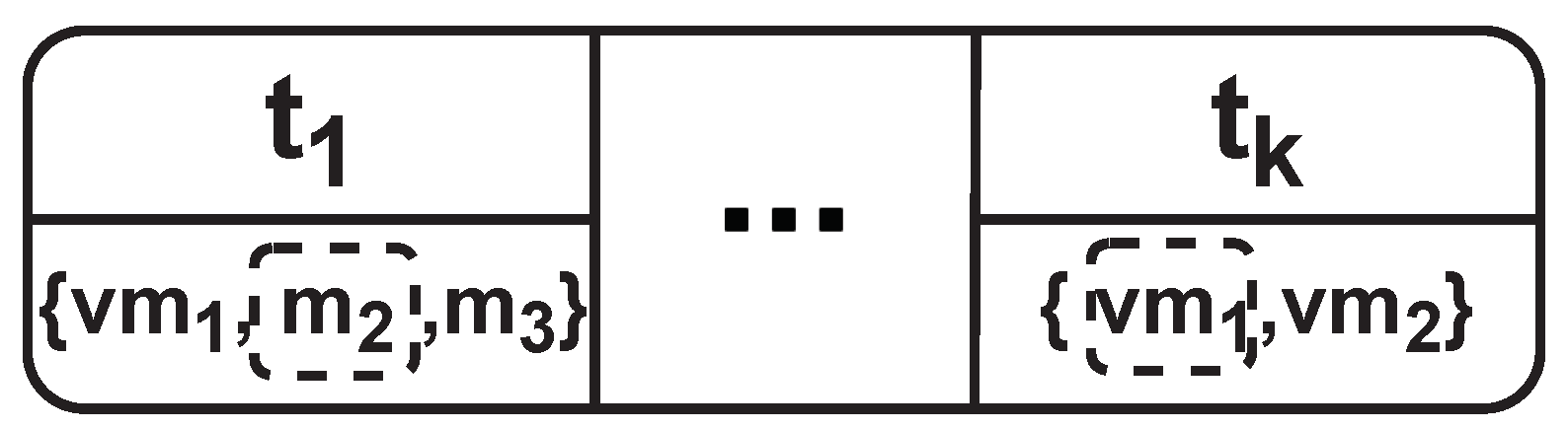
A particle structure in the algorithm that is shown in Figure 4 has a dynamic length equal to the number of available jobs at time τ , and each job is assigned to either an edge server ( m i ) or a public cloud virtual machine ( v m j ). This selection relies on a candidate list ( α t i ) per each job resource requirement ( R i t ).
The initial population ( P ) is begun with an eligible permutation of job resource selection. There is a list ( β ) that maintains resource availability across the edge-cloud environment. Each job in the workload (T) is checked for preparing a list of servers and/or virtual machines that can host a job. The list relies on the edge utilization level in which edge servers are descendingly sorted based on the utilization level (both CPU and memory) at time τ . The list of each job is capped at | T | + 1 servers to avoid computation overhead caused by PSO. Moreover, a job candidate list is updated by adding a temporarily idle server from the I list of the edge. This added server would be confirmed if current active servers could not satisfy a job’s resource requirement. Moreover, if a job is privacy-sensitive, it has to choose the edge servers. Otherwise, both edge servers and public cloud virtual machines are taken into account.
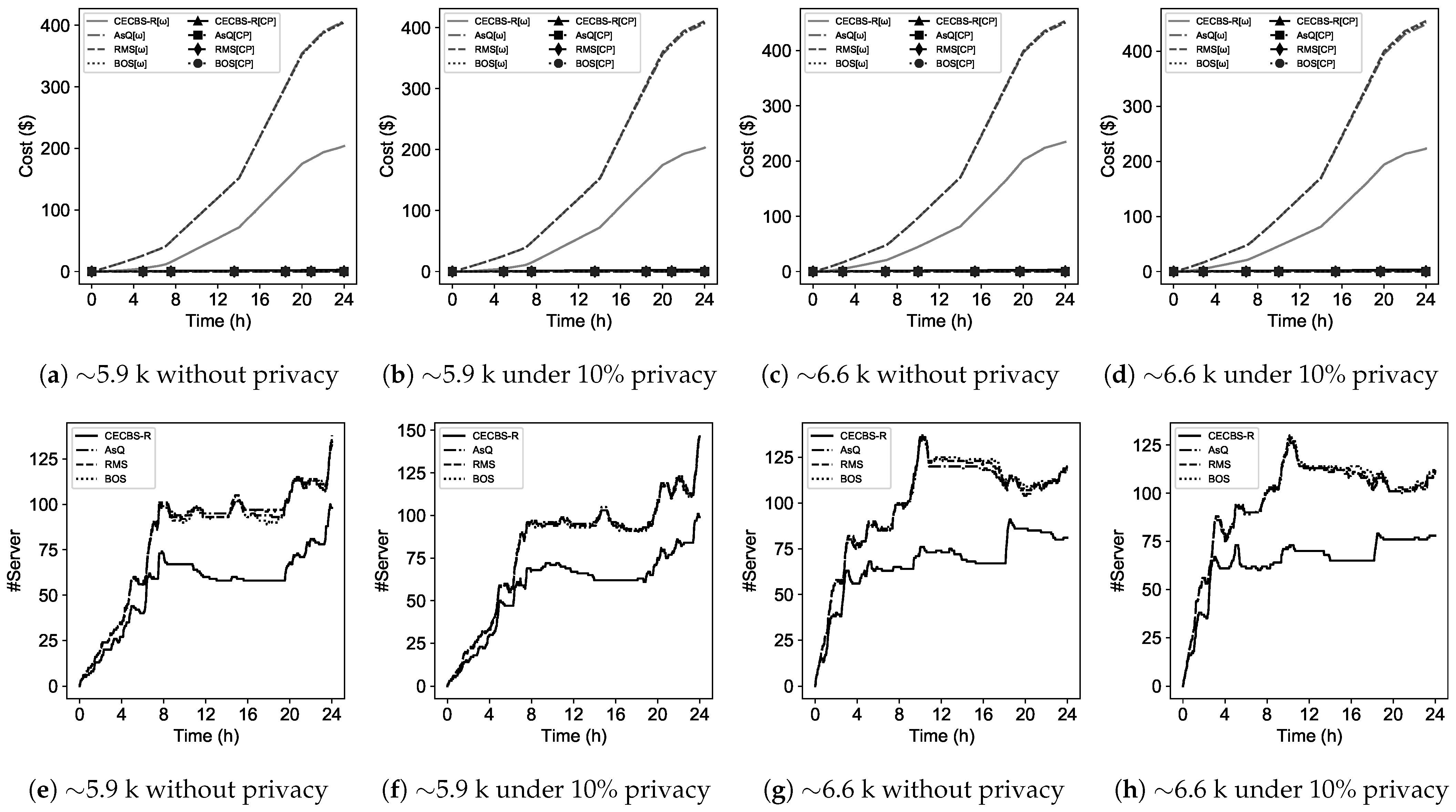
When CECBS-R works as the scheduler, Algorithm 2 considers estimated runtimes to assist the selection of cost-efficient resources. Otherwise, it will seek feasible recommendations to schedule jobs onto resources in the edge-cloud environment. In other words, if a regular job is recommended to be scheduled onto the edge with no available servers, the recommended cloud is updated based on the most cost-efficient resources with respect to Equation (8) that considers billing cycles, and the estimated runtime ( E R T i t ) across the edge-cloud environment.
Per each resource candidate list of a job ( α t i ), the population is updated by mapping a selected resource to a job for forming a solution. Each solution is evaluated against a fitness function for cost-efficiency and the quality of resource assignment. When a job ( t i ) is assigned to a candidate resource (m or v m ), its resource candidate list ( α t i ) and the resource availability list ( β ) are updated. If during the process, α t i becomes empty, the backup candidate list ( α t i b ) will update the list.
The quality of each particle ( ρ ) is assessed by the fitness function ( f ρ ) that consists of controlling and quality parameters, each of which evaluates a particular aspect of the particle. Controlling parameters are defined as the cloud priority ( ρ ϱ ) and the job resource allocation ( ρ ς ).
A particle may have jobs that are assigned to public cloud virtual machines, however, there should be a mechanism to prioritize edge resource selection. In other words, jobs should be avoided to be processed on the public clouds while the edge has sufficient resources available. Hence, ρ ϱ checks jobs in the particle and penalizes the fitness with ψ [ 0 , 1 ] , in which the edge has lower penalized value compared to public clouds, i.e., ψ R < ψ R C P .
ρ ϱ = i = 0 ρ ψ i
Moreover, jobs in a particle should be checked, whether or not the chosen server (m) or the virtual machine ( v m ) can satisfy jobs resource requirements ( R i t ). It is expressed as ρ ς that returns t r u e or f a l s e if the resource requirement is satisfied or not, respectively.
The quality parameters should control the edge utilization ( ρ κ ) and the estimated cost ( ρ ζ ). If jobs are assigned to servers in the edge, it should have to increase the overall utilization. Therefore, a particle ( ρ ) is assessed against how chosen servers ( m i ) can contribute toward better utilization.
ρ κ = i = 0 ρ U T i
Finally, the estimated cost of a particle ( ρ ) for cost-efficiency is computed in Equation (16). The cost is divided into two parts; the edge and public clouds. The former cost is directly affected by the impact of utilization level on the energy consumption as the higher utilization leads towards the higher energy consumption, and consequently, the higher fitness ratio. In contrast, the latter has a reverse impact on the fitness function, since it aims to reduce the reliance on public cloud resources.
( ρ ζ ω , ρ ζ E C ) = i = 0 ρ E C ω R i t R . i = 0 ρ E C C P O t h e r w i s e .
If a server of the edge is assigned to a job ( t i ), ρ ζ ω will consider the electricity cost based on the utilization that the server will have. Otherwise, it will compute the usage cost of virtual machines in public clouds based on the billing cycle.
The fitness function based on the controlling and quality parameters is defined as follows.
f ρ = ρ ς × ρ κ × ρ ζ ω ρ ϱ × ρ ζ E C
In the fitness function, if the denominator is increased, the fitness function will lead toward particles that are not cost efficient. This is due to leaving the edge resources under-utilized and relying more on public clouds. If the numerator is increased and becomes aligned with a small denominator, the fitness function will lead to expressing solutions that are cost efficient and will improve the edge resource utilization.
The PSO algorithm through each iteration updates the best local ( P l c ) and global ( P g b ) known positions. These positions are the chosen resource indexes in the corresponding candidate list ( α t i ) shown in Figure 5. In order to generate new solutions based on the current population, particles should have to move in the search space with respect to the swarm movement terminology. The movement is controlled by a particle location ( L ρ i ) and its speed ( V ρ i ). Each particle updates its location ( L ρ i ) and its velocity ( V ρ i ) with respect to the P l c and P g b , stated in Equations (18) and (19), respectively. The velocity of a particle ( V ρ i ) is also controlled by the PSO learning parameters referred to as c 1 , c 2 , and { ξ , θ } [ 0 , 1 ] [30].
V ρ i = θ × V ρ i + c 1 × ξ × ( P l c L ρ i ) + c 2 × ξ × ( P g b L ρ i )
L ρ i = L ρ i + V ρ i
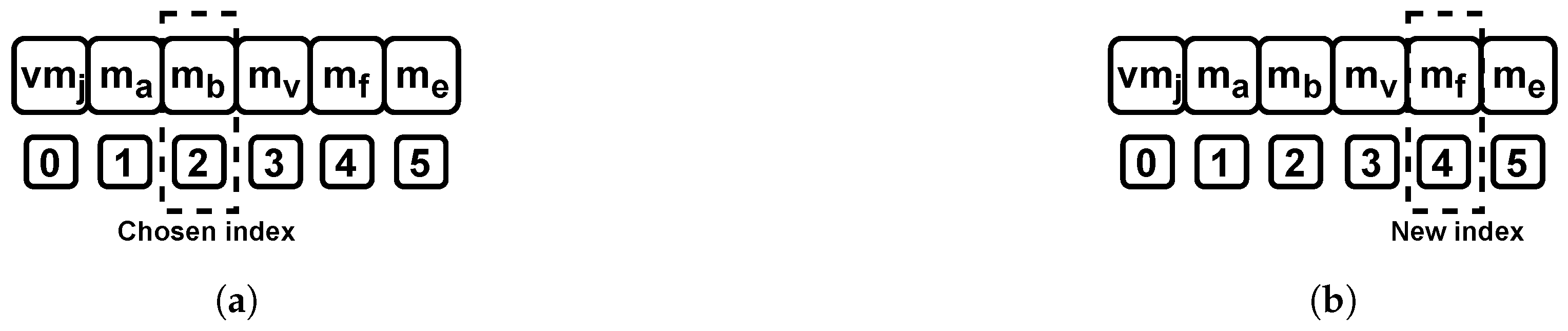
Velocities in the cloud scheduler (Algorithm 2) are the candidate index positions in α t i for job t i . Hence, locations are bounded in the length of | α t i | that is updated per new index position provided by the new velocity.
L ρ j t i = L ρ j t i + V ρ j t i V ρ j | α t i | L ρ j t i + V ρ j t i % | α t i | O t h e r w i s e .
Equation (20) shows that when the updated velocity ( V ρ j t i ) in ρ j exceeds the length of α t i , it will return the reminder as the new index for choosing a new candidate. Figure 5 illustrates that if the current index for job t i in α t i is 2, the updated velocity V ρ j t i { | α t i | × n } ( n N ) will change the location.

3.3. CECBS-R Time Complexity

CECBS-R employs a PSO algorithm for scheduling jobs in the edge that consults with the cloud state controller algorithm to seek recommendations/classification. The PSO fitness function affects the algorithm running time, which relies on the number of jobs available at time τ that also impacts the population size. In other words, if the PSO has N p populations to become evaluated in G i iteration, the PSO will converge in O ( N p · G i ) steps.
Moreover, the worst-case upper bound of running time for mapping recommended jobs ( l o f f ) to cost-efficient public clouds depends on the cost comparison between the clouds. If there are | C P | public clouds, the running time is stated as O ( | l o f f | · | C P | ) . Hence, CECBS-R requires the following running time for T jobs at time τ :
max T ( O ( N p · G i ) , O ( | l o f f | · | C P | ) )

4. Evaluation

In this section, we evaluate the performance of the CECBS-R framework in terms of server usage, QoS violations (i.e., missing deadlines), and cost in comparison to BOS [6], RMS [5], and AsQ [22]. For the baseline algorithms, actual runtimes are available in advance. BOS is a policy-driven hybrid scheduler to maximize utilization while reducing the usage cost of public clouds. It uses two queue management policies, such as first-come-first-served (FCFS) and earliest deadline first (EDF), which are accompanied by two offloading policies referred to as unfeasible and the cheapest jobs to the public clouds. The EDF queue policy, in conjunction with the unfeasible offloading policy, is used for comparison. RMS also maintains the job queues which are managed by heterogeneous earliest finish time (HEFT) algorithm for cost-efficient resource allocation to the jobs leading to performance improvement. AsQ is an optimization algorithm that aims at scheduling deadline-constrained jobs to improve utilization while reducing public cloud rental costs.
The comparison is reported in two separate sections based on the edge server usage, cost, and QoS violations. The first section compares the CECBS-R scheduler against baseline algorithms, and the results are used to build up datasets for training the recommender. The second section shows the result of the CECBS-R recommender compared to the mentioned algorithms.

4.1. Simulation Setup

The edge-cloud in our experiment consists of an edge and four recognized public cloud providers; Amazon Web Services, Microsoft Azure, Google Cloud Engine, and Alibaba Cloud. Public cloud VMs are chosen on-demand from the US East region and their types are selected from general-purpose and compute-optimized VMs. The VMs are subject to charges based on the billing policy (i.e., per hour vs. per second), and this charge considers bandwidth and storage usage. The deployment time of each public cloud provider on average is 100 s for AWS [31], 90 s for Microsoft Azure [32], 90 s for Alibaba cloud, and 54 s for Google Cloud Engine [33].
It is assumed that the edge has a cluster of 200 servers similar to a large private IBM cloud infrastructure [34]. Each server has 64GB memory and a dual processor (18 cores) running at 3300 million instructions per second (MIPS). Moreover, each server under different utilization levels requires an estimated wattage usage that is shown in Table 2. Off-peak, shoulder, and peak electricity rates are $12.08196, $51.04627, and $24.44365 kilowatts per hour [35], respectively.
We use Facebook Hadoop traces [20] and public grid workload traces [21] as inputs for our simulation, and jobs are synthesized to be short, medium, and long-running jobs with a ratio of 75:20:5 [15]. Jobs are assigned a length in MIPS and follow a Gaussian distribution with respect to (mean, variance) values that are (1, 10), (10, 100), and (100, 1000) for short, medium, long-running jobs, respectively. Resource requirements for jobs are shown in Table 3 and jobs are categorized into interactive and delay-insensitive groups with 27:73 ratio [15] under relaxed user-defined deadline ratios chosen from [ 0.1 , 0.5 ] and [ 0.5 , 1.0 ] , respectively. Moreover, jobs follow non-preemptive scheduling, and results are reported for non-privacy jobs and 10% of interactive jobs to be privacy-sensitive.
Particle swarm optimization parameters are considered the default values; 2 for both c 1 , c 2 , and θ is 0.8 and 5% of edge servers are assumed to be initially active. The initial population size is dynamic and is assumed to be a coefficient of incoming jobs and their chosen resources at time τ capped at 200. The generation size ( G i ) is considered 200.

4.1.1. Server Management Datasets & Parameters

CECBS-R uses virtual machine utilization traces to train the RNN-based server management implemented in Keras; the Python deep learning API [36], and traces are chosen distributed data center performance metrics from Bitbrains composed of 1750 VMs [37]. CECBS-R uses the time interval 60 s for the edge server states and 300 s for checking the job state in the edge-cloud environment [15]. Although VMware introduces 30 s (low), 60 s (medium), and 120 s (high) time intervals, it states that the high and low sensitivity intervals may cause a false or long detection [38]. The RNN has three layers in which the hidden layer has 64 neurons. The input of the RNN is the CPU and memory utilization, as well as overall server utilization that each input belongs to a utilization category; low (under 20%), medium (between 20% and 80%), and high (higher than 80%) [15].
The RNN leverages hyperbolic tangent activation function ( t a n h ) for the hidden layer and softmax for the output layer. Furthermore, the training dataset is divided into two sets—training and validation—with a ratio of 80:20 under 100 epochs.
To validate the RNN model for server management, F1-score is reported as a measure of accuracy. The value considers precision and recall for computing the score. The former reports the ratio of correct positive divided by all positive results returned by the classifier. The latter is the ratio of correct positive results divided by the number of all relevant samples. In essence, the higher F1-score emphasizes how perfect the model is. In addition, the loss is reported that shows how well the ANN performs on the training and validation datasets.
Figure 6 shows the overview of training loss and F1-score over 100 epochs (i.e., based on subtle changes in the error ratio) and illustrates the significant accuracy of the model. The F1-score for the server management proves the performance of the designed classifiers; increasing or decreasing the edge servers with respect to the servers’ load.

4.1.2. RNN versus Vanilla Server Management

To show how effective the ANN-assisted server management is, a comparison between the RNN model and a vanilla strategy for controlling the servers in the edge is reported. The vanilla strategy takes into account the CPU utilization level at the specified interval and sends a signal with respect to the server utilization level.
We ran CECBS-R based on a crafted trace consisting of ∼13.3 k jobs under the privacy of 10% in which jobs inherit Facebook dataset characteristics, but with a different job arrival time for 24 h. The comparison based on the edge cost and server usage is depicted in Figure 7.
Figure 7a illustrates that the vanilla server management gradually became expensive during the execution time (i.e., ∼3% more expensive), with average costs of $407 and $413 for RNN and vanilla, respectively. Moreover, although they almost achieved the same server usage (on average 135), Figure 7b shows that RNN followed more steady usage patterns than vanilla, resulting in cheaper execution cost for the edge. Recall that the RNN-assisted server management takes into account both CPU, RAM, and overall cluster utilization for the purpose of sending a controlling signal. In contrast, vanilla server management only considers CPU utilization, which could blindly turn on or off servers.

4.1.3. Runtime Estimation Datasets and Parameters

The runtime estimation model employs a four-layer MLP neural network with tanh activation function. The input layer receives job characteristics, such as requested memory and CPU core, the length, actual runtime, and the CPU speed of the server or VM where it is executed. The MLP has 64 neurons for hidden layers, which are followed by the output layer. It is a one-hot vector associated with the duration controller ( γ i ) that represents a coarse-grained classification.
The MLP neural network is trained under 100 epochs based on grid workload datasets which consist of more than 1 million jobs logged for two months [39]. CECBS-R relies on the ∼5-day of unseen datasets to collect job execution information across the edge-cloud to be fed into the network (recall Section 2.2.1). Figure 8 shows the overview of training loss and F1-score which is followed by the validation’s values. The loss provides a small model error that shows the data is perfectly fitted into the designed model for the runtime estimation. Moreover, the F1-score is high, meaning low false positives and false negatives identified in this model training.

4.2. The Scheduler Results

This section presents results for workload scheduling by CECBS-R compared to the baseline algorithms. CECBS-R heuristically schedules jobs across the edge-cloud environment, taking into account runtime uncertainties managed by the MLP neural network. In contrast, the baseline algorithms considering virtually accurate runtimes are available in advance.
Table 4 presents different workloads’ characteristics that are used for this section. The traces contain job information and resource requirements unless otherwise it is stated. The synthesized workloads are crafted based on the measured arrival time between consecutive jobs in the real Facebook traces; ∼5.9k and ∼6.6k. The average arrival time between jobs is reported as 14, hence, to craft new workloads out of the real workloads, the arrival time is chosen from the following set— { 7 , 10 , 14 } —which creates ∼11.6 k, ∼15.8 k, and ∼21.7 k synthesized traces. These synthesized traces are assigned new resource requirements with respect to Table 3. Moreover, CECBS-R reports the results of another public trace workload composed of nearly 4 consecutive days of job submission [21].
We start by presenting the accumulated edge and public cloud cost for traces ∼5.9 k and ∼6.6 k during the execution time of a day followed by the edge server usage. Figure 9 shows the overall accumulated cost when jobs have no privacy and have a privacy ratio of 10% along with edge server usage. This figure illustrates that the accumulated cost is impacted by increasing the number of jobs, the privacy ratio, and the corresponding type of jobs. Comparing Figure 9a,b shows that CECBS-R achieved nearly the same edge cost, which is less than the cost of the other algorithms. This is supported by Figure 9e,f. In these figures, CECBS-R utilized the edge servers aligned with the workload assisted by the machine learning server management, taking advantage of public clouds, in particular, AWS. While AsQ and BOS almost have the same cost and less cost than RMS, CECBS-R maintained cheaper workload execution. In Figure 9c, CECBS-R also maintained a lower cost than the baseline algorithms which can be supported by Table 5 as CECBS-R leveraged public clouds (i.e., AWS) resources for workload execution. Furthermore, Figure 9g,h motivate the fact that controlling the edge server usage with respect to the incoming workload can significantly improve the overall edge utilization. For a higher privacy ratio, CECBS-R sent off jobs to the public clouds compared to the other algorithms led to achieving the less cost shown in Figure 9d and Table 5. This table shows the total execution cost across the edge-cloud environment and the contribution of each/cloud environment to this cost. It is understood that the edge cost has the highest contribution to the cost, and the value is the minimum for CECBS-R.
Increasing the number of jobs in traces (Figure 10) changed the accumulated cost across the edge-cloud environment, as well as the edge server usage. The usage of public clouds also became more obvious, in particular, for Figure 10c,d. This shows that CECBS-R achieved the least total edge-cloud cost in comparison to the other algorithms through maintaining the execution workload within the edge. It is expected that it will result in higher server usage, which is clear in Figure 10e–h. Increasing the privacy ratio made the internal resources on the edge busier, therefore, it would be more cost efficient to schedule jobs on the resources across the edge-cloud environment. While CECBS-R barely had information about the accurate runtimes in comparison to the baseline algorithm, it could achieve lower edge cost (Figure 10a,b), which is also aligned with the server usage in Figure 10e,f. Furthermore, in Table 5(a), CECBS-R, on average, utilized more edge resources, leading to maintaining lower public cloud cost, which emphasizes better resource allocation for the privacy ratios. Increasing the server utilization while the idle servers become deactivated (i.e., put in deep sleep mode) reduced the edge cost significantly for CECBS-R.
Increasing the number of jobs in traces (Figure 11) resulted in increasing the edge cost for all algorithms (Table 5(a)–(e)), which is also related to the number of jobs becoming available at a specific time (recall Figure 9 and Figure 10). This is seen in Figure 11e–h. However, CECBS-R used fewer servers compared to other algorithms for scheduling and leveraged fewer servers less than 48 h. The more jobs become available for scheduling, the more servers are required; in particular, for privacy-sensitive jobs.
Table 5 shows that CECBS-R took advantage of public clouds and controlling the active servers to achieve cost efficiency. In contrast, all the baseline algorithms used the edge inefficiently, which led to higher costs that are also emerged from poor server management of the edge. Although the edge cost for CECBS-R is the lowest, the total cost of scheduling for ∼61 k jobs is the most among all algorithms. To investigate this, we present the number of QoS violations (i.e., number of missed deadlines) that happened for the traces in Table 6. This table presents that CECBS-R could reduce the number of QoS violations when the number of jobs increased. Although AsQ has the least total cost under privacy ratios, it has the highest violated QoS. BOS and RMS almost achieved the same cost after AsQ, with significantly fewer violations, but still higher than CECBS-R.
CECBS-R for ∼61 k trace relied more on public clouds (Table 5) for offloading purposes to comply with the QoS. In contrast, the heuristic-based CECBS-R scheduler led to a lower cost for the edge. The public cloud usage shows that CECBS-R considers the cost efficiency of resources on public clouds, while considering the active servers in the edge. Furthermore, AsQ, RMS, and BOS leveraged all the available servers inside the edge earlier than CECBS-R and achieved higher cost, while CECBS-R used fewer servers within the edge for half of a day. In fact, knowing runtimes without considering how cost-efficient it is to use either edge or public resources cannot lead to cost-saving.
Figure 12 shows the total cost when jobs have no privacy (Figure 12a) and under privacy ratios of 10% (Figure 12b) and illustrates that CECBS-R outperformed other algorithms. Even for the workload trace with the size of ∼61 k, CECBS-R could perform better than AsQ, because the number of QoS violations is the least for the CECBS-R shown in Table 6.

4.3. The Recommender Results

In this section, the result of CECBS-R recommender for an unseen and new Facebook workload trace (∼24.45 k jobs), as well as Karlsruhe Institute of Technology (KIT) System trace (∼44.5 k jobs) [40] across the edge-cloud environment is reported. The former is the real workload trace for 24 h while the latter is the traces collected over one year and a half in which the last four months of the trace are selected for this section. For recommendation, CECBS-R is trained by the previous scheduling results obtained from the CECBS-R scheduler under the given privacy ratios.
The CECBS-R recommender employs an LSTM neural network that consists of three layers. The input layer receives job submission time, length, required CPU cores and memory, privacy, deadline, the corresponding electricity rates category, and the edge utilization level at the time of job scheduling. The output is a one-hot vector associated with the job’s cloud environment. Moreover, the training datasets are divided into two sets, with a ratio of 80:20 for training and validation, respectively.
Figure 13 shows the overall training error and the F1-score for the model validation considering the previous job executed information. The loss and F1-score for the resource recommender with respect to the collected job information show that the model could learn a diverse job resource allocation, as the training error is still low. This figure is followed by the re-trained MLP neural network (Figure 14) for runtime estimation taking into account the executed job information across the edge-cloud environment. Due to the job diversities within the workloads, the F1-score for the validation set is almost ∼85%, which could still be leveraged for the recommendation. The model is retrained with the new collected job information, meaning that the designed model should have to be re-adjusted, hence, it is expected to have an increment in the model error, and a lower F1-score for the runtime estimation. Figure 15 shows that considering the recommendation eventually led to cost efficiency with the least QoS violations. Although AsQ could achieve the least cost for the trace ∼24.4 k without privacy, the CECBS-R could guarantee the QoS of jobs slightly at a higher cost than AsQ.
Figure 15c,d shows how CECBS-R utilized edge servers better than the other algorithms. For the trace contains ∼24.45 k jobs, AsQ, RMS, and BOS almost used all the servers in the edge towards the end of execution, however, nearly a quarter of the time CECBS-R used fewer resources than the other algorithms. This resulted in different edge costs for the baseline algorithms and CECBS-R. While CECBS-R relied on the recommendations, on average, it achieved a lower edge cost than the other algorithms when jobs have no privacy and under a 10% privacy ratio. Although CECBS-R sent off more jobs to the edge (Table 5(a)), it effectively used the resources which led to cost efficiency because of being helped by the PSO algorithm. The usage of edge servers could increase the chance of relying on the public cloud for job execution (Figure 15a,b). However, for CECBS-R, the heuristic fitness function Equation (17) recommended that jobs were executed in the edge aimed at increasing resource utilization, while achieving a lower cost. Higher server utilization would increase the wattage usage with respect to Equation (4); consequently, it would increase the usage cost, but at the same time, underutilized servers would also hurt the cost-efficiency, as idle servers in a data center consume 50% of peak power [41,42].
Figure 16 shows that CECBS-R assisted by neural networks achieved the lowest cost for longer traces and comparing to other algorithms when privacy is in effect, CECBS-R relied on the public resources (see Table 7). In contrast, AsQ, RMS, and BOS relied on edge resources for job execution and hardly ever used public clouds. Table 7a (and Table 7(b)–(e)) show that after CECBS-R, RMS almost sent off more jobs to the edge, and AsQ offloaded more jobs to the public clouds for the trace ∼24.4 k. CECBS-R for higher privacy ratios steadily tended to employ both edge and public resources, in particular, relying more on the edge servers. It should be noted that even with the availability of runtimes in advance for baseline algorithms, the scheduler/recommender plays an important part in making judicious scheduling decisions, as baseline algorithms could not achieve cost efficiency for any of the traces.
Table 7 shows that CECBS-R outperformed the baseline algorithms, as CECBS-R could learn what resources would be more cost-efficient across the edge-cloud environment. It can be seen that CECBS-R leveraged public resources (Table 7(a)–(e)) for the trace ∼44.5 k, as it was cost efficient to use resources there. CECBS-R could perfectly be aligned with the workload pattern as comparing Figure 15c,d with Figure 16 shows that the usage of the edge could be close to the baseline algorithm but in a more efficient way. Less spikes can be seen in Figure 16 for CEBCS-R, e.g., days ∼27, ∼40, ∼70, and ∼105. Recall the fact that leaving edge resource underutilized (or idle) could lead to increasing the utility cost which can be seen in Table 7. Consequently, cloud bursting recommendations based on LSTM significantly reduced the total cost across the edge-cloud environment. These results show how CECBS-R could recommend better judicious decisions based on the learnt workload characteristics and their resource requirements for achieving cost savings that are aligned with Figure 15, Figure 17 and Figure 18. Moreover, Table 8 shows the number of QoS violations for CECBS-R and the other algorithms as for ∼44.5 trace CECBS-R slightly violated more jobs’ QoS.

5. Related Work

Cloud bursting has been extensively studied [12,22,43,44,45,46,47,48,49,50,51] and studies [5,6,7,8,52,53,54,55,56,57,58] pay attention to scheduling for improving cost and/or performance. However, a majority of studies fail to notice the impact of the edge (i.e., in situ resources) utility cost in cost efficiency, while preserving privacy. Moreover, due to the presence of workload runtime uncertainties, the cost-efficiency of cloud bursting becomes more challenging, but can be addressed through applying machine learning techniques for resource selection or recommendation [15,17].
Calheiros’ work [5] is about deadline-constraint job scheduling, in which job queues and resource queues are used to allocate resources for deadline-sensitive or deadline-insensitive jobs. Cost optimization can be found in [7,8,44,49,51]. In these works, performance [7,44,49] and minimizing the public cloud cost [8,51] are studied considering the improvement of local resource utilization. Chen et al. [52] present how cost evaluation can be effective for choosing off-premise resources. Bossche et al., [54,56] show the potential cost-efficient cloud environment selection for deadline-constraint jobs through cost evaluation. He also, in another study [6], developed a four-strategy algorithm that cost-effectively manages submitted jobs to the edge to be executed across a hybrid cloud. The developed online hybrid scheduler leverages two offloading policies for resource selection for the public cloud, as well as two job selection strategies for incoming jobs at the edge when they are deadline-sensitive.
As CECBS-R is assisted by ML techniques and employs edge-cloud resources, it falls in the context of cyber-physical systems (CPSs) [59], where the risk assessment (i.e., preserving privacy, e.g., user data) is controlled through the proper allocation of resources across the edge while meeting incoming jobs’ resource requirements [60]. Moreover, due to the complexities of cloud bursting for software products, Acs et al. [12] offer a nested virtualization technique to seamlessly overcome the issues and the cloud differences. The usage of a data locality for iterative MapReduce applications through cloud bursting [43], a heuristic approach for task sequencing and task scheduling for minimizing bags-of-task completion, and through binary linear programming [55], includes research works in cost-efficient resource allocation. Furthermore, Chunlin et al. [47] address resource-intensive mobile application scheduling, which leverages service-level agreement (SLA) to determine the share of both edge and public clouds resources to be allocated to a mobile user.
Data-driven approaches have also gained attention for resource allocation [46,48,50,61]. In [46], a support vector machine (SVM) is used to profile and anticipate user activities for resource management in a multimedia cloud environment, and [48] proposes a framework that relies on the processing time estimations to feasibly allocate resources to jobs. Champati et al. [50] discuss an online runtime estimation-based algorithm to efficiently minimize makespan in the edge while keeping the offloading minimum, and Sonmez et al. [61] presented a two-stage machine learning-based load orchestrator for task allocation in edge/cloud servers.
Optimal resource allocation which leads to cost-efficiency are studied through a multi-dimension knapsack problem [22] and Pareto-optimality [53,62]. Charrada and Tata [57] propose a cost calculation strategy for resource selection based on procedure-based approaches, while bursting workloads to the public cloud.
Although these studies address cloud bursting cost efficiency and/or dealing with workload surges, neither workload privacy nor the utility cost is considered. Hence, this paper not only considers the edge utility cost and workload privacy, but also takes advantage of machine learning techniques to facilitate cloud bursting for achieving better cost efficiency. Therefore, this paper is distinguishable from the studies above, as the edge utility cost under various electricity rates is taken into account for job scheduling under privacy constraints. Machine learning techniques are used to deal with runtime uncertainties and assist cloud bursting for choosing the cost-efficient cloud/edge environment, which is done by learning job characteristics and resource requirements.

6. Conclusions

This paper has studied the cost efficiency of AI-assisted scheduling in the edge-cloud environment with the development of CECBS-R as a dual-objective framework for scheduling and recommendation. CECBS-R incorporated machine learning techniques such as MLP, LSTM, and LSTM neural networks that were responsible for learning, training, and recommendation in the edge-cloud environment. CECBS-R not only preserved privacy, but also considered the edge utility cost plus public cloud billing cycles for scheduling for cost-efficient scheduling. Moreover, CECBS-R by profiling jobs assisted scheduling through resource recommendations as well as runtime estimation. CECBS-R is trained with the scheduling outputs of Facebook and grid workload traces as real workload traces. CECBS-R has shown that considering the advantages of the edge-cloud environment can lead to cost efficiency, and a resource recommender could be in charge of the cost-efficient resource allocation. Results under different scenarios compared to the state-of-the-art algorithms have confirmed our claims. For our future work, resource-constrained devices in addition to the heterogeneous resources across the edge-cloud environment will be considered to provide more insights into their contribution to resource allocation.

Author Contributions

Formal analysis, A.P., Y.C.L., T.H. and K.A.; Methodology, A.P.; Project administration, Y.C.L.; Supervision, Y.C.L.; Validation, Y.C.L., T.H. and K.A.; Writing—original draft, A.P.; Writing—review and editing, A.P. and Y.C.L. All authors have read and agreed to the published version of the manuscript.

Funding

This research received no external funding.

Data Availability Statement

No new data were created or analyzed in this study. Data sharing is not applicable to this article.

Conflicts of Interest

The authors declare no conflict of interest.

References

  1. Amazon EC2 Pricing. 2020. Available online: https://aws.amazon.com/ec2/pricing/ (accessed on 21 May 2021).
  2. Microsoft Azure Pricing. 2020. Available online: https://azure.microsoft.com/en-au/pricing/ (accessed on 21 May 2021).
  3. Google Compute Engine. 2020. Available online: https://cloud.google.com/compute/pricing (accessed on 21 May 2021).
  4. Alibaba Cloud. 2020. Available online: https://www.alibabacloud.com (accessed on 21 May 2021).
  5. Calheiros, R.N.; Buyya, R. Cost-Effective Provisioning and Scheduling of Deadline-Constrained Applications in Hybrid Clouds. In Web Information Systems Engineering—WISE 2012; Wang, X.S., Cruz, I., Delis, A., Huang, G., Eds.; Springer: Berlin/Heidelberg, Germany, 2012; pp. 171–184. [Google Scholar]
  6. Den Bossche, R.V.; Vanmechelen, K.; Broeckhove, J. Online cost-efficient scheduling of deadline-constrained workloads on hybrid clouds. Future Gener. Comput. Syst. 2013, 29, 973–985. [Google Scholar] [CrossRef]
  7. Bittencourt, L.F.; Senna, C.R.; Madeira, E.R. Scheduling service workflows for cost optimization in hybrid clouds. In Proceedings of the 2010 International Conference on Network and Service Management (CNSM), Izmir, Turkey, 2–6 November 2010; pp. 394–397. [Google Scholar]
  8. Lee, Y.; Lian, B. Cloud Bursting scheduler for cost efficiency. In Proceedings of the 10th IEEE International Conference on Cloud Computing, Honolulu, HI, USA, 25–30 June 2017; pp. 774–777. [Google Scholar]
  9. Clemente-Castelló, F.J.; Mayo, R.; Fernández, J.C. Cost Model and Analysis of Iterative MapReduce Applications for Hybrid Cloud Bursting. In Proceedings of the 2017 17th IEEE/ACM International Symposium on Cluster, Cloud and Grid Computing (CCGRID), Madrid, Spain, 14–17 May 2017; pp. 858–864. [Google Scholar]
  10. Chu, H.; Simmhan, Y. Cost-Efficient and Resilient Job Life-Cycle Management on Hybrid Clouds. In Proceedings of the 2014 IEEE 28th International Parallel and Distributed Processing Symposium, Phoenix, AZ, USA, 19–23 May 2014; pp. 327–336. [Google Scholar]
  11. Hoseinyfarahabady, M.R.; Samani, H.R.D.; Leslie, L.M.; Lee, Y.C.; Zomaya, A.Y. Handling Uncertainty: Pareto-Efficient BoT Scheduling on Hybrid Clouds. In Proceedings of the 2013 42nd International Conference on Parallel Processing, Lyon, France, 1–4 October 2013; pp. 419–428. [Google Scholar]
  12. Acs, S.; Kozlovszky, M.; Kacsuk, P. A novel cloud bursting technique. In Proceedings of the 2014 IEEE 9th IEEE International Symposium on Applied Computational Intelligence and Informatics (SACI), Timisoara, Romania, 15–17 May 2014; pp. 135–138. [Google Scholar]
  13. Ilyushkin, A.; Epema, D. The Impact of Task Runtime Estimate Accuracy on Scheduling Workloads of Workflows. In Proceedings of the 2018 18th IEEE/ACM International Symposium on Cluster, Cloud and Grid Computing (CCGRID), Washington, DC, USA, 1–4 May 2018; pp. 331–341. [Google Scholar]
  14. Soysal, M.; Berghoff, M.; Klusáček, D.; Streit, A. On the quality of wall time estimates for resource allocation prediction. In Proceedings of the 48th International Conference on Parallel Processing: Workshops, Kyoto, Japan, 5–8 August 2019; pp. 1–8. [Google Scholar]
  15. Cortez, E.; Bonde, A.; Muzio, A.; Russinovich, M.; Fontoura, M.; Bianchini, R. Resource Central: Understanding and Predicting Workloads for Improved Resource Management in Large Cloud Platforms. In Proceedings of the 26th Symposium on Operating Systems Principles, Shanghai, China, 28–31 October 2017; ACM: New York, NY, USA, 2017; pp. 153–167. [Google Scholar]
  16. Microsoft Azure Traces. 2019. Available online: https://github.com/Azure/AzurePublicDataset (accessed on 21 May 2021).
  17. Yadwadkar, N.J.; Hariharan, B.; Gonzalez, J.E.; Smith, B.; Katz, R.H. Selecting the Best VM Across Multiple Public Clouds: A Data-driven Performance Modeling Approach. In Proceedings of the 2017 Symposium on Cloud Computing, Santa Clara, CA, USA, 24–27 September 2017; ACM: New York, NY, USA, 2017; pp. 452–465. [Google Scholar]
  18. Duc, T.L.; Leiva, R.G.; Casari, P.; Östberg, P.O. Machine Learning Methods for Reliable Resource Provisioning in Edge-Cloud Computing: A Survey. ACM Comput. Surv. 2019, 52. [Google Scholar] [CrossRef] [Green Version]
  19. Pasdar, A.; Lee, Y.C.; Almi’ani, K. Toward Cost Efficient Cloud Bursting. In Service-Oriented Computing; Yangui, S., Bouassida Rodriguez, I., Drira, K., Tari, Z., Eds.; Springer International Publishing: Cham, Switzerland, 2019; pp. 299–313. [Google Scholar]
  20. Facebook Workload Traces. 2019. Available online: https://github.com/SWIMProjectUCB/SWIM/wiki/Workloads-repository (accessed on 21 May 2021).
  21. Grid Workload. 2020. Available online: http://gwa.ewi.tudelft.nl/datasets/gwa-t-11-lcg (accessed on 21 May 2021).
  22. Wang, W.J.; Chang, Y.S.; Lo, W.T.; Lee, Y.K. Adaptive scheduling for parallel tasks with QoS satisfaction for hybrid cloud environments. J. Supercomput. 2013, 66, 783–811. [Google Scholar] [CrossRef]
  23. Power Supply Calculator. 2019. Available online: https://outervision.com/power-supply-calculator (accessed on 21 May 2021).
  24. Beloglazov, A.; Abawajy, J.; Buyya, R. Energy-aware resource allocation heuristics for efficient management of data centers for cloud computing. Future Gener. Comput. Syst. 2012, 28, 755–768. [Google Scholar] [CrossRef] [Green Version]
  25. Lim, S.H.; Sharma, B.; Tak, B.C.; Das, C.R. A dynamic energy management scheme for multi-tier data centers. In Proceedings of the (IEEE ISPASS) IEEE International Symposium on Performance Analysis of Systems and Software, Austin, TX, USA, 10–12 April 2011; IEEE: New York, NU, USA, 2011; pp. 257–266. [Google Scholar]
  26. Fan, X.; Weber, W.D.; Barroso, L.A. Power provisioning for a warehouse-sized computer. ACM SIGARCH Comput. Archit. News 2007, 35, 13–23. [Google Scholar] [CrossRef]
  27. Reiss, C. Towards understanding heterogeneous clouds at scale: Google trace analysis. In Proceedings of the Third ACM Symposium on Cloud Computing, San Jose, CA, USA, 23–25 October 2012. [Google Scholar]
  28. Energy Australia. 2019. Available online: https://www.energyaustralia.com.au/business/electricity-and-gas/small-business/plans (accessed on 21 May 2021).
  29. Goodfellow, I.; Bengio, Y.; Courville, A. Deep Learning; MIT Press: Cambridge, MA, USA, 2016; Available online: http://www.deeplearningbook.org (accessed on 21 May 2021).
  30. Wang, D.; Tan, D.; Liu, L. Particle swarm optimization algorithm: An overview. Soft Comput. 2018, 22, 387–408. [Google Scholar] [CrossRef]
  31. Mao, M.; Humphrey, M. A performance study on the vm startup time in the cloud. In Proceedings of the 2012 IEEE Fifth International Conference on Cloud Computing, Honolulu, HI, USA, 24–29 June 2012; pp. 423–430. [Google Scholar]
  32. Microsoft Azure Deployment Time. 2019. Available online: https://feedback.azure.com/forums/216843-virtual-machines/suggestions/5715040-accelerate-vm-startup-time (accessed on 21 May 2021).
  33. Google Compute Engine Deployment Time. 2019. Available online: https://medium.com/google-cloud/understanding-and-profiling-gce-cold-boot-time-32c209fe86ab (accessed on 21 May 2021).
  34. Sizing Your IBM® Cloud Private Cluster. 2019. Available online: https://www.ibm.com/support/knowledgecenter/en/SSBS6K_3.1.2/installing/plan_capacity.html (accessed on 21 May 2021).
  35. Energy Australia: Energy Price Fact Sheet NSW Business (Elec-Tricity). 2017. Available online: https://secure.energyaustralia.com.au/EnergyPriceFactSheets/Docs/EPFSIE_B_N_BBAS_EA_6_02-01-2017.pdf (accessed on 21 May 2021).
  36. Keras Python Deep Learning API. 2020. Available online: https://keras.io (accessed on 21 May 2021).
  37. Bitbrains VMs Performance. 2019. Available online: http://gwa.ewi.tudelft.nl/datasets/gwa-t-12-bitbrains (accessed on 21 May 2021).
  38. VMware, Inc. 2019. Available online: https://www.vmware.com/au.html (accessed on 21 May 2021).
  39. Grid Workload. 2020. Available online: http://gwa.ewi.tudelft.nl/datasets/gwa-t-1-das2 (accessed on 21 May 2021).
  40. Karlsruhe Institute of Technology Workload Traces. 2019. Available online: https://www.cs.huji.ac.il/labs/parallel/workload/l_kit_fh2/index.html (accessed on 21 May 2021).
  41. Greenberg, A.; Hamilton, J.; Maltz, D.A.; Patel, P. The Cost of a Cloud: Research Problems in Data Center Networks. SIGCOMM Comput. Commun. Rev. 2008, 39, 68–73. [Google Scholar] [CrossRef]
  42. Barroso, L.A.; Hölzle, U. The Case for Energy-Proportional Computing. Computer 2007, 40, 33–37. [Google Scholar] [CrossRef]
  43. Clemente-Castello, F.J.; Nicolae, B.; Rafique, M.M.; Mayo, R.; Fernandez, J.C. Evaluation of Data Locality Strategies for Hybrid Cloud Bursting of Iterative MapReduce. In Proceedings of the 2017 17th IEEE/ACM International Symposium on Cluster, Cloud and Grid Computing (CCGRID), Madrid, Spain, 14–17 May 2017; pp. 181–185. [Google Scholar]
  44. Loreti, D.; Ciampolini, A. A Hybrid Cloud Infrastructure for Big Data Applications. In Proceedings of the 2015 IEEE 17th International Conference on High Performance Computing and Communications, 2015 IEEE 7th International Symposium on Cyberspace Safety and Security, and 2015 IEEE 12th International Conference on Embedded Software and Systems, New York, NY, USA, 24–26 August 2015; pp. 1713–1718. [Google Scholar]
  45. Zhang, Y.; Sun, J.; Wu, Z. An Heuristic for Bag-of-Tasks Scheduling Problems with Resource Demands and Budget Constraints to Minimize Makespan on Hybrid Clouds. In Proceedings of the 2017 Fifth International Conference on Advanced Cloud and Big Data (CBD), Shanghai, China, 13–16 August 2017; pp. 39–44. [Google Scholar]
  46. Daniel, D.; Raviraj, P. Distributed Hybrid Cloud for Profit Driven Content Provisioning Using User Requirements and Content Popularity. Cluster Comput. 2017, 20, 525–538. [Google Scholar] [CrossRef]
  47. Chunlin, L.; Jianhang, T.; Youlong, L. Distributed QoS-aware scheduling optimization for resource-intensive mobile application in hybrid cloud. Cluster Comput. 2018, 21, 1331–1348. [Google Scholar] [CrossRef]
  48. Zhu, J.; Li, X.; Ruiz, R.; Xu, X. Scheduling Stochastic Multi-Stage Jobs to Elastic Hybrid Cloud Resources. IEEE Trans. Parallel Distrib. Syst. 2018, 29, 1401–1415. [Google Scholar] [CrossRef]
  49. Zuo, L.; Shu, L.; Dong, S.; Chen, Y.; Yan, L. A Multi-Objective Hybrid Cloud Resource Scheduling Method Based on Deadline and Cost Constraints. IEEE Access 2017, 5, 22067–22080. [Google Scholar] [CrossRef]
  50. Champati, J.P.; Liang, B. One-restart algorithm for scheduling and offloading in a hybrid cloud. In Proceedings of the 2015 IEEE 23rd International Symposium on Quality of Service (IWQoS), Portland, OR, USA, 15–16 June 2015; pp. 31–40. [Google Scholar]
  51. Guo, T.; Sharma, U.; Wood, T.; Sahu, S.; Shenoy, P. Seagull: Intelligent cloud bursting for enterprise applications. In Proceedings of the 2012 {USENIX} Annual Technical Conference ({USENIX}{ATC} 12), Boston, MA, USA, 13–15 June 2012; pp. 361–366. [Google Scholar]
  52. Chen, Y.; Sion, R. To Cloud or Not to Cloud? Musings on Costs and Viability. In Proceedings of the 2nd ACM Symposium on Cloud Computing, Cascais, Portugal, 23–25 October 2011; ACM: New York, NY, USA, 2011; p. 29. [Google Scholar]
  53. Farahabady, M.R.H.; Lee, Y.C.; Zomaya, A.Y. Pareto-Optimal Cloud Bursting. IEEE Trans. Parallel Distrib. Syst. 2014, 25, 2670–2682. [Google Scholar]
  54. Den Bossche, R.V.; Vanmechelen, K.; Broeckhove, J. Cost-Optimal Scheduling in Hybrid IaaS Clouds for Deadline Constrained Workloads. In Proceedings of the 2010 IEEE 3rd International Conference on Cloud Computing, Miami, FL, USA, 5–10 July 2010; pp. 228–235. [Google Scholar]
  55. Abdi, S.; PourKarimi, L.; Ahmadi, M.; Zargari, F. Cost Minimization for Deadline-constrained Bag-of-tasks Applications in Federated Hybrid Clouds. Future Gener. Comput. Syst. 2017, 71, 113–128. [Google Scholar] [CrossRef]
  56. Den Bossche, R.V.; Vanmechelen, K.; Broeckhove, J. Cost-Efficient Scheduling Heuristics for Deadline Constrained Workloads on Hybrid Clouds. In Proceedings of the 2011 IEEE Third International Conference on Cloud Computing Technology and Science, Athens, Greece, 29 November–1 December 2011; pp. 320–327. [Google Scholar]
  57. Charrada, F.B.; Tata, S. An Efficient Algorithm for the Bursting of Service-Based Applications in Hybrid Clouds. IEEE Trans. Serv. Comput. 2016, 9, 357–367. [Google Scholar] [CrossRef]
  58. Li, C.; Tang, J.; Luo, Y. Towards operational cost minimization for cloud bursting with deadline constraints in hybrid clouds. Cluster Comput. 2018, 21, 2013–2029. [Google Scholar] [CrossRef]
  59. Radanliev, P.; De Roure, D.; Van Kleek, M.; Santos, O.; Ani, U. Artificial intelligence in cyber physical systems. AI Soc. 2020, 1–14. [Google Scholar] [CrossRef]
  60. Radanliev, P.; De Roure, D.; Walton, R.; Van Kleek, M.; Montalvo, R.M.; Santos, O.; Burnap, P.; Anthi, E.; others. Artificial intelligence and machine learning in dynamic cyber risk analytics at the edge. SN Appl. Sci. 2020, 2, 1–8. [Google Scholar] [CrossRef]
  61. Sonmez, C.; Tunca, C.; Ozgovde, A.; Ersoy, C. Machine Learning-Based Workload Orchestrator for Vehicular Edge Computing. IEEE Trans. Intell. Transp. Syst. 2021, 22, 2239–2251. [Google Scholar] [CrossRef]
  62. Ben-Yehuda, O.A.; Schuster, A.; Sharov, A.; Silberstein, M.; Iosup, A. ExPERT: Pareto-Efficient Task Replication on Grids and a Cloud. In Proceedings of the 2012 IEEE 26th International Parallel and Distributed Processing Symposium, Shanghai, China, 21–25 May 2012; pp. 167–178. [Google Scholar]
Figure 1. Structure of CECBS-R.
Information 12 00224 g001
Figure 2. The volatile electricity categories per day stated by Energy Australia [28]. Each square presents a time of day.
Information 12 00224 g002
Figure 3. ANN types. (a) A three-layer feed-forward network that takes inputs and produces two outputs. (b) RNN neural network in which the hidden layer output returns to the network. (c) LSTM cell with four gates in which • is Hadamard product and ∫ is the activation function.
Information 12 00224 g003
Figure 4. The particle structure. The dashed square is the selected resource.
Information 12 00224 g004
Figure 5. A ti candidate list ( α t i ) with 5 edge servers { m a , m b , m v , m f , m e } and one public cloud VM ( v m j ). (a) Already chosen index before updating the location. (b) After updating the location considering 2 for V ρ j t i .
Information 12 00224 g005
Figure 6. The loss and F1-score over 100 epochs for the RNN server management.
Information 12 00224 g006
Figure 7. RNN versus vanilla server management.
Information 12 00224 g007
Figure 8. The loss and F1-score over 100 epochs for the runtime estimation model.
Information 12 00224 g008
Figure 9. The accumulated edge ( ω ) and public cloud ( C P ) cost followed by the edge server usage for ∼5.9 k and ∼6.6 k jobs.
Information 12 00224 g009
Figure 10. The accumulated edge ( ω ) and public cloud ( C P ) cost followed by the edge server usage for ∼11.6 k and ∼15.8 k jobs.
Information 12 00224 g010
Figure 11. The accumulated edge ( ω ) and public cloud ( C P ) cost followed by the edge server usage for ∼21.7 k and ∼61 k jobs.
Information 12 00224 g011
Figure 12. The total cost across the edge-cloud environment without privacy and under 10% privacy.
Information 12 00224 g012
Figure 13. The loss and F1-score over 100 epochs for the recommender.
Information 12 00224 g013
Figure 14. The loss and F1-score over 100 epochs for the runtime estimation model.
Information 12 00224 g014
Figure 15. The accumulated edge ( ω ) and public cloud ( C P ) cost followed by the edge server usage for ∼24.4 k jobs.
Information 12 00224 g015
Figure 16. The edge server usage for ∼44.5 k jobs during 3 months.
Information 12 00224 g016
Figure 17. The accumulated edge ( ω ) and public cloud ( C P ) cost for ∼44.5 k jobs.
Information 12 00224 g017
Figure 18. The total cost across the edge-cloud environment without privacy and under 10% privacy.
Information 12 00224 g018
Table 1. Symbol description.
SymbolDescription
M C An edge-cloud environment
C P Cloud provider
R/ R C P Set of edge/public cloud resources
B C i Billing cycle of cloud provider i
B C i a / B C i n Active/New billing cycle of cloud provider i
E C Estimated cost of a cloud
v m i A public cloud virtual machine
m j An edge server
U T i Utilization of the edge server i
ω i Expected wattage usage of edge server i
R i t Required resources of job i
D i t Deadline of job i
R C i t Recommended cloud env. of job i
A R T i t Actual runtime of job i
E R T i t Estimated runtime of job i
E C i t Estimated cost of job i
B / S Set of cloud provider charges for bandwidth/storage
A / I Set of active/idle servers in the edge
d j The coarse-grained duration i
Table 2. Utilization wattage requirement ( w a t t ) [23].
0%10%20%30%40%50%60%70%80%90%100%
188223258293328363398433468503538
Table 3. Resource requirements [17].
(a) #Cores.
Job percentage<55%<20%<10%<3%<4%<2%<3%<2%<1%
CPU cores1246812202432
(b) Memory (GB).
Job percentage<5%<38%<4%<20%<3%<10%<2%<10%<8%
Memory0.751.7523.504781416/28/32–64
Table 4. Workload traces.
TraceType# Jobs in TraceDuration
FacebookReal∼5.9 k24 h
FacebookReal∼6.6 k24 h
FacebookSynthesized∼11.6 k24 h
FacebookSynthesized∼15.8 k24 h
FacebookSynthesized∼21.7 k24 h
GridReal∼61k∼4 days
Table 5. Edge-cloud job proportion and its cost under volatile ( ω v ) electricity rates.
(a) Edge
TracePrivacyJob ProportionCost ($)
CECBS-RAsQRMSBOSCECBS-RAsQRMSBOS
∼5.9 k5760589558955895203.82406.98405.44404.71
∼5.9 k10%5767589558955895203.11407.20410.89408.80
∼6.6 k6492663966396639234.71450.70453.69451.30
∼6.6 k10%6488663966396639223.37448.92454.93452.17
∼11.6 k11,57811,57811,56811,568356.71570.73570.63570.63
∼11.6 k10%11,57811,57811,50311,503362.61557.97556.49556.49
∼15.8 k15,77412,86215,10915,109475.61642.62618.36618.36
∼15.8 k10%15,77412,68314,90114,901493.94638.16614.92614.92
∼21.7 k21,23415,31519,28619,286604.29661.35642.78642.78
∼21.7 k10%21,26515,33618,47318,473609.74660.35637.67637.67
∼61 k53,12834,95245,97545,5222182.222437.222378.282382.69
∼61 k10%52,48537,90033,22433,2092189.012439.092389.772381.63
(b) AWS
TracePrivacyJob ProportionCost ($)
CECBS-RAsQRMSBOSCECBS-RAsQRMSBOS
∼5.9 k1350002.79000
∼5.9 k10%1260002.96000
∼6.6 k1470003.11000
∼6.6 k10%1510003.37000
∼11.6 k00000000
∼11.6 k10%00000000
∼15.8 k046966024.21.671.67
∼15.8 k10%0428121204.937.267.26
∼21.7 k21138944448.9147.9919.0119.01
∼21.7 k10%6125685854.2916.2325.9625.96
∼61 k40063818699733224.17230.08194.79168.03
∼61 k10%4006375223322159218.26265.61187.25185.36
(c) GCE
TracePrivacyJob ProportionCost ($)
CECBS-RAsQRMSBOSCECBS-RAsQRMSBOS
∼5.9 k00000000
∼5.9 k10%00000000
∼6.6 k00000000
∼6.6 k10%00000000
∼11.6 k00000000
∼11.6 k10%0022001.281.28
∼15.8 k0211010012.5210.4710.47
∼15.8 k10%0352222030.3740.4340.43
∼21.7 k0393636027.2874.474.4
∼21.7 k10%0684747055.1996.5896.58
∼61 k12720015415564.43125.73335.77328.67
∼61 k10%193213218225105.45317.79356.81384.11
(d) MS
TracePrivacyJob ProportionCost ($)
CECBS-RAsQRMSBOSCECBS-RAsQRMSBOS
∼5.9 k00000000
∼5.9 k10%00000000
∼6.6 k00000000
∼6.6 k10%00000000
∼11.6 k0088001.921.92
∼11.6 k10%0058580024.5324.53
∼15.8 k02334464464070.46169.77169.77
∼15.8 k10%02438630630054.35162.13162.13
∼21.7 k316469518251825350.28134.87290.04290.04
∼21.7 k10%314459425292529458.64148.37384.22384.22
∼61 k196220,94212,22012,6653885.62170.281987.231970.62
∼61 k10%216817,23523,00623,2084156.681283.981645.171728.8
(e) AC
TracePrivacyJob ProportionCost ($)
CECBS-RAsQRMSBOSCECBS-RAsQRMSBOS
∼5.9 k00000000
∼5.9 k10%20000.14000
∼6.6 k00000000
∼6.6 k10%00000000
∼11.6 k0022001.431.43
∼11.6 k10%0015150010.8710.87
∼15.8 k088185185089.39385.97385.97
∼15.8 k10%01902092090177.72289.37289.37
∼21.7 k88222469469130.84234.691147.251147.25
∼21.7 k10%7440652652697.36607.791148.021148.02
∼61 k17781089195319264177.811118.635144.15090.34
∼61 k10%21491901222122004517.074438.225457.135469.17
Table 6. #QoS violations.
TracePrivacyCECBS-RAsQRMSBOS
∼5.9 k0000
10%0000
∼6.6 k0000
10%0000
∼11.6 k0500
10%02700
∼15.7 k0131600
10%011613030
∼21.7 k0384800
10%103409103103
∼61 k0∼15.9 k00
10%254∼17.1 k646507
Table 7. Edge-cloud job proportion and its cost under volatile ( ω v ) electricity rates.
(a) Edge
TracePrivacyJob ProportionCost ($)
CECBS-RAsQRMSBOSCECBS-RAsQRMSBOS
∼24.4 k20,87218,82619,55919,495638.95669.75645.64647.01
∼24.4 k10%20,90516,59423,14417,939639.6670.77647.71645.56
∼44.5 k42,85344,46644,46644,4664994.9640,550.9840,572.2840,527.96
∼44.5 k10%42,86844,46644,46644,4665334.4340,589.1240,600.6640,356.52
(b) AWS
TracePrivacyJob ProportionCost ($)
CECBS-RAsQRMSBOSCECBS-RAsQRMSBOS
∼22.4 k2434108429925348.8101.5673.1452.62
∼22.4 k10%228914561456348.4687.62102.0590.66
∼44.5 k114800073.55000
∼44.5 k10%115000087.83000
(c) GCE
TracePrivacyJob ProportionCost ($)
CECBS-RAsQRMSBOSCECBS-RAsQRMSBOS
∼24.4 k52751069513.9765.06151.66129.49
∼24.4 k10%551272311413.66111.02171.95179.75
∼44.5 k6500061.89000
∼44.5 k10%6000017.9000
(d) MS
TracePrivacyJob ProportionCost ($)
CECBS-RAsQRMSBOSCECBS-RAsQRMSBOS
∼24.4 k570412835923706672.12568.24662.63676.89
∼24.4 k10%62954819764929633.12444.3553.46642.21
∼44.5 k173000181.68000
∼44.5 k10%162000198.84000
(e) AC
TracePrivacyJob ProportionCost ($)
CECBS-RAsQRMSBOSCECBS-RAsQRMSBOS
∼24.4 k515330887894591.59504.151951.811932.87
∼24.4 k10%565785286898635.021273.62085.92006.55
∼44.5 k227000307.9000
∼44.5 k10%226000396.51000
Table 8. #QoS violations.
TracePrivacyCECBS-RAsQRMSBOS
∼24.4 k0423500
10%634886146137
∼44.5 k10000
10%8000
Publisher’s Note: MDPI stays neutral with regard to jurisdictional claims in published maps and institutional affiliations.

