Abstract
Navigation in a traffic congested city can prove to be a difficult task. Often a path that may appear to be the fastest option is much slower due to congestion. If we can predict the effects of congestion, it may be possible to develop a better route that allows us to reach our destination more quickly. This paper studies the possibility of using a centralized real-time traffic information system containing travel time data collected from each road user. These data are made available to all users, such that they may be able to learn and predict the effects of congestion for building a route adaptively. This method is further enhanced by combining the traffic information system data with previous routing experiences to determine the fastest route with less exploration. We test our method using a multi-agent simulation, demonstrating that this method produces a lower total route time for all vehicles than when using either a centralized traffic information system or direct experience alone.
1. Introduction
When a driver attempts to navigate in a modern urban environment, they must overcome many obstacles to reach their destination, e.g., poor weather, road construction and accidents; however, while these problems may occur with varying degrees of frequency, traffic congestion is one which is encountered daily. Delays on the morning and evening commute to and from work are familiar to many who regularly travel in a city. Indeed, in particularly congested cities with high population densities, the problem of traffic congestion may be a constant condition on many roads.
Delays due to traffic congestion can be the cause of many problems. Drivers experience increased stress as delays may cause them to miss appointments or arrive late for work. Environmental damage is also a concern, as traffic delays require vehicles to operate for longer periods than may otherwise be necessary, resulting in increased pollution due to automotive exhaust. As well, economic damage can occur as worker productivity is reduced due to increased stress and work time lost in travel [1].
When one considers the negative impacts of congestion its reduction would be beneficial both to individuals and society. However, reducing congestion is not a simple task. Building additional roads to increase the volume of traffic that may be handled without congestion may not be possible in many locations, due to existing structures or budget constraints. Increased availability of mass transit can be helpful in reducing the number of road users, but this can be expensive to operate and may not be feasible for users who must travel beyond a short distance to reach their destination. If we consider that many commuters may opt to drive personal vehicles, either by preference or necessity, it is worthwhile to investigate how they may be better routed to reach their destinations while minimizing the negative effects of congestion. The simplest approach to routing is to take the shortest path to one’s destination. While this may seem ideal, the shortest path may not be the best option, as the roads selected may have a low speed limit and thus be inherently slow. The roads may also be congested at the time of travel, causing the route to be slower than anticipated. A more sophisticated approach to routing would involve a consideration of the speed limit on each road taken. By factoring in how fast we can travel on each road in our path, we can calculate how long it would take to travel them. As such, a path that uses faster roads may result in a shorter route time than one that simply selects the shortest path. These routing methods are examples of user or individually optimized routing [2]. This type of routing focuses on finding the fastest, or optimal, route to the driver’s destination. As such, there is little regard for the impact on existing traffic congestion beyond the necessity to limit its effects in delaying the driver. However, using individually optimized routing can have a detrimental effect when all drivers attempt to use this method. Referred to as the tragedy of the commons [3], this problem appears when all vehicles attempt to use the same roads at the same time. As the road is finite in the number of vehicles that may efficiently use it concurrently, increasing the number of users will increase the amount of time it takes to travel upon the road.
An alternate method is to build routes that are system optimized. System optimization focuses on reducing the total amount of travel time for all vehicles using the road network [2], with the goal of reducing the impact of each vehicle on the congestion problem. As such, many road networks are designed to favor system optimization by operating high capacity and high-speed roads, with the goal of moving the largest number of vehicles possible through the system. System optimization can also be attempted with traffic light systems that prioritize traffic on high capacity roads while also directing vehicles towards them [2]. Unfortunately, system optimization may result in negative effects for some drivers. When a route is built to take advantage of high capacity roads, the driver may not be using the best route to reach their destination—they may be required to take a longer path than otherwise necessary. While this can reduce the total travel time experienced by all drivers—the modified path reduces congestion on some other road—the individual driver does not see a benefit.
Ideally, we would like to optimize the route for the individual while also optimizing for the system. A hybrid method, combining both individual and system optimized routing attempts to use the best components of both methods to achieve this [2]. By selecting roads that provide for a fast route for the driver but also work to avoid congestion, we can avoid building routes that cost the individual too much time while also working to reduce the total congestion in the road network. The reduction in congestion may then be enough to offset the extra time that the individual driver must spend reaching their destination. However, when routing in congestion, one must consider the following question: is it better for me to use a road that is short, but congested? or, is it better for me to take a road that is longer, but uncongested? The answer to this question is not simple when one does not know how badly congested the road is, as a short but congested road may be a better option than a longer, uncongested one if the delay due to congestion is small.
To see if we can develop routes that are better suited for areas with traffic congestion than existing methods, we consider:
- (1)
- Finding the best route while accounting for congestion requires the driver to search through several possible alternatives.
- (2)
- The specific amount of congestion that will be encountered on any given road segment is unknown to the driver.
- (3)
- Avoiding the tragedy of the commons to approach a system optimum state.
Finding the fastest route to one’s destination can be accomplished using several pathfinding algorithms, such as Dijkstra’s Algorithm [4] or the A* algorithm [5]. Given a map with sufficient detail of the road segment lengths and permissible road speeds, these algorithms can provide a route that will get the driver to their destination; however, given the unknown details of congestion and its effects on road speed, these algorithms are insufficient by themselves.
If we were to use a pathfinding algorithm to produce several possible routes that our driver could choose from, we may be able to find the fastest route. To do this we can use reinforcement learning to try to learn which route will be the quickest. Multi-Armed Bandit algorithms (MAB) [6,7,8] can be used to search for the best routing solution and more reliably select it in the future. However, to learn the fastest route to take, these methods must first explore the possible solutions, resulting in the driver using some potentially poor routes while trying to find the best one. Thus, Objective 1 of our research is to determine the fastest route for the driver with the least exploration.
Second, as the amount of congestion along a given route affects its speed, if a driver would like to select the fastest route with a limited number of routing tries, more detailed information about the congestion on a road segment may be of help. Software such as Google Traffic [9] and Waze [10] offer information about the traffic conditions on a road. Both operate by collecting data from public traffic sensors and user provided travel times (via smartphone application) and use it to provide routes that account for delays due to congestion. While a large amount of travel data can be collected from users, we must consider that the congestion problem will change over time. The number of road users may change, and the routes they select can result in roads becoming congested over time. As such, we need a routing method that can adapt to changes in congestion and anticipate what these changes will do to congestion while building a route. Thus, our Objective 2 is to propose a routing method that can adapt to changes in congestion over successive routing actions.
As mentioned above, the tragedy of the commons occurs when each driver attempts to select the fastest route without regard for the effects of this selection on congestion. Ideally, we would like to avoid this issue and reach a system optimum state where the total travel time is at a minimum while also minimizing the travel time for each driver. Stackelberg routing [11], where a leader is selected to pick an initial route which is then built upon by others, can be used to solve this issue; however, this method requires a central authority to select the leader and assign routes, which may or may not be followed by the other drivers if they consider them to be unfair. This provides us with Objective 3, that is, to construct a routing method that produces routes that are fair for each driver but also minimizes the total travel time for all drivers.
This research makes multiple contributions towards solving the congestion problem in the urban environment:
- First, we show that the fastest route in a congested road network can be determined with less exploration than might otherwise be necessary. This is achieved by combining the data the driver acquires through experience driving a route with the data that are collected by all road users.
- Second, we show that this method is adaptable to changes in the congestion problem by constructing a new reinforcement-learning-based approach to teaching each driver which travel data best matches the current congestion.
- Finally, we demonstrate, by a multi-agent simulation, that the drivers can reach an equilibrium point that approaches the system optimum while being directed through a control mechanism.
The term agent is used to refer to the vehicle’s navigation system. The agent develops the routes and decides which one the vehicle will take. The driver of the vehicle managed by the vehicle simulation and will always follow the route provided by the agent. The term road segment is used to refer to a section of a road that lies between two intersections. As the routing agent can only make road selection decisions at an intersection, the road segment represents the smallest unit of a road that the agent can perceive. The travel time refers to the time, in seconds, required for a vehicle to travel the length of a road segment. The travel time may be that of an individual vehicle or may be an average of all vehicles for a specified range of times.
The rest of the paper is organized as follows: Section 2 reviews the literature on the routing methods. Section 3 discusses the theoretical foundation for the proposed methods. Section 4 covers the design of the solution and the method of experimentation. Section 5 presents our experimental results. Section 6 discusses the results of this research. Finally, Section 7 presents the conclusions and future work.
2. Literature Review
To optimize the road network, Intelligent Transportation Systems (ITS) [12,13] focuses on using traffic information to make better use of existing infrastructure. Centralized traffic management systems, such as the Sydney Coordinated Adaptive Traffic System (SCATS) [14] attempt to improve traffic flow by further managing traffic lights, such that busier roads are given priority to increase the speed of vehicles traveling along the road when there is high traffic volume. While this technology can greatly improve traffic flow, it is complex and costly to implement. As well, changing traffic light timings to favor certain roads will encourage drivers to prefer using them, resulting in further congestion.
Recent advances in communications technology have also enabled the use of more advanced techniques. Vehicle-to-roadside (V2R) communications technologies allow for greater organization of the network by transmitting information about destination and vehicle status to local traffic management systems [15]. Intelligent intersections can sense the volume and direction of traffic passing through them and time signal changes to improve flow while also providing information to neighboring intersections about the volume of traffic headed in their directions [12,15,16].
Many routing methods attempt to solve the routing problem by focusing on reaching either a User Equilibrium (UE) or System Optimum (SO) state [17]. Each of these principles may be understood intuitively as the consequences of either self-interested or altruistic agents [18].
Game theory is used to model the problem of traffic congestion in a city, representing the problem as a congestion game [19,20]. The game reaches equilibrium when no player perceives a possibility of improving their reward by changing strategy [21]. The game theory analysis of routing in traffic congestion views the problem as a nonatomic congestion game consisting of many players attempting to use a set of roads [20]. As the number of players is very large, although not infinite, the decisions of any individual player on the congestion encountered is very small—essentially, the decision of any one player to use a particular road at a particular time will not make a noticeable difference in how fast a vehicle may travel down that road. A common example of this class of game is the El Farol Bar Problem [20].
There have been a few different approaches that have been applied to the routing problem. These approaches can be separated into attempting to solve for either of Wardrop’s Principles or both [17], with varying levels of sophistication. Perhaps the most direct method of routing is to select a path that combines the fastest allowable road speeds with the shortest possible distance. Provided a map of the city in which we would like to navigate, we can use a pathfinding algorithm such as Dijkstra’s Algorithm [4] or A* [5].
Route Information Sharing (RIS) [22] represents one method to reach a system optimum. By sharing information on the routes chosen by drivers, this method seeks to enable them to avoid congestion. Route information sharing has been shown to provide an improvement in the average travel time for drivers using this method over the average times for drivers routing using a shortest distance method. This difference was found to increase as the percentage of vehicles using RIS increased in the road network. However, while an improvement was found, the number of cycles of route, transmit, receive and re-route that must be accomplished before a final set of routes is reached can be large. As well, it has been noted that, in large cities where there may be millions of vehicles, such a system may be impractical, as a typical communications system, such as a cellular network, may not capable of handling the number of connections required.
While a system-optimal method of routing results in faster overall route times, it is difficult to prevent the system from reverting to a less-efficient user equilibrium state. RIS approaches this; however, it does so at the price of potentially delayed routing results and a large communications infrastructure cost. If drivers are selfish in their behaviors (that is, always attempting to achieve the fastest route for themselves, regardless of the cost to others), perhaps a better approach would be to achieve a user equilibrium state that is as close as possible to the social optimum. Levy et al. [18,23] investigate the possibility of system optimum being an emergent property of a multi-agent system. In their research, a group of agents, representing drivers, are given a choice between two routes of equal length. As both routes are equal, the only factor that affects the route completion time is the number of agents that select the route. Each agent has the goal of reaching the end of the route in the shortest time possible and must decide which route is the best choice to achieve this. The authors solve this problem by applying the agents’ previous routing experience on each route. A routing simulation was built for the agents with both available routes. As successive simulations are run, the agents acquired more information as to the amount of time required to complete each route, which is used to inform the agent’s route selection in the next simulation. To determine which route is likely to be the least congested, each agent uses the Sampling and Weighting (SAW) formula [24]. While this work shows that it is possible to reach a user equilibrium and a social optimum state using a deterministic algorithm, there are some practical limitations. First, the agents required almost 2000 runs to reach a user equilibrium, and reaching a social optimum required approximately 500 runs. If such a system were attempted for a group of drivers, it would require a large number of tries before they saw a significant improvement in their route times. Secondly, the experiments gave the agents the option of two routes, rather than the hundreds that may be possible in an urban road network. Given the larger number of options, a weight value that accounts for long-term memory may result in a better result than that was found when only two routes were allowed.
The multi-armed bandit framework [25] has been used to model and simulate sequential route selection or generation problems. Recently, Zhou et al. [26] formulated a sequential route selection problem as a shortest path problem with on-time arrival reliability under a multi-armed bandit setting. The upper confidence bound algorithm is extended to handle this problem [26]. The objective of their application is to identify the arm with both the shortest travel time and most likely to arrive on time. The goal of our research is to predict the effects of congestion and develop a better route that allows us to reach our destination more quickly. Yoon and Chow [27] proposed a sequential route generation process for line planning and route generation under uncertainty for public transit network design. A reinforcement learning-based route generation methodology is proposed to support line planning for emerging technologies. The method makes use of contextual bandit problems to explore different routes to invest in while optimizing the operating cost or demand served [27]. While their research is focusing on public transit network design, our paper is focusing on individual vehicle navigation.
3. The Theoretical Framework
We present a multi-agent routing methodology that addresses the objectives of the research. To develop their route, each agent uses the following steps: first, the agent builds a list of potential routes to its destination. The list is built using a modified version of the A* algorithm, which returns the fastest routes possible based on the map data available to the agent. For all potential routes in the list, the agent estimates the time at which they will start each road segment. Next, the agent requests travel time data from the centralized real-time traffic information system (TIS) for each road segment in each route. By using the TIS, the agent avoids the need to try each route to learn the amount of congestion firsthand, thus minimizing the exploration required to estimate its effects. The TIS returns two average travel times for each road segment requested, adjusted for the time at which the agent estimates it will reach the segment: the first is the long-term average, which is an average of all vehicle travel times on the given road segment for all available routing episodes; second, the short-term average, comprised of the average travel time for all vehicles in a certain number of most recent routing episodes. The agent then applies the averages to each potential route using the SAW formula. The agent selects the route with the fastest estimated time. As the estimates are developed using previous travel time data, our routing method can adapt to changes in congestion—the effects of any changes will be reflected in the travel times used. The agent compares the selected route to a list of routes it has traveled previously. If the route is the same as the route used by the agent in the previous routing episode, the agent will select the route. If it is different, the agent searches the list to determine if it has used the route before. If not, the agent will use the route. If the agent has used the route previously, it will only select the new route if it was significantly faster than the route used in the previous routing episode.
The agent travels its route. As the agent travels, it transmits the time required to complete each road segment to the TIS. If re-routing is enabled for the agent, it compares the time on route to its estimated route time to that point. If the route time is significantly higher than the estimated time it will re-route. After completing its route, the agent reviews the route times for each of its potential routes by again querying the TIS to apply the most recent travel time data to each one. If the fastest route was different than the one the agent selected, they adjust their selection algorithm to better reflect the effects of congestion on its routes. As each agent acts to improve its route selection, the amount of time to complete its routes are reduced and works to minimize the total travel time for all drivers, while also providing a fair route for the agent. Figure 1 presents a flowchart depicting the agent’s routing actions. The algorithm Agent Routing Process provides an overview of the agent routing steps and calls the algorithms presented in the following sections.
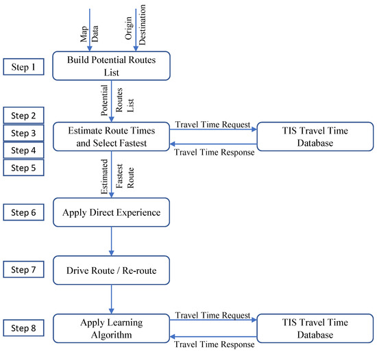
Figure 1.
Agent routing process.
3.1. Building the Potential Routes List (Step 1)
Before selecting the fastest path to its destination, the agent must first develop a list of viable routes. In many cities the number of possible routes can be quite large, given a multitude of roads to choose from; however, many routes are not good options due to a combination of allowable road speed and distance. To accomplish this task, the agent uses a modified version of the A* algorithm [5]. Our modified version will continue to build routes until a pre-determined number of routes has been reached, providing the agent with a list of routes to choose from.
Given a list of potential routes, the agent must now determine which one to use while also accounting for the effects of congestion. As shown by Levy et al. [18,23], determining the impact congestion has on a given route can require a large number of tries before we can be sure we have found the fastest one. To reduce the amount of searching required to find the fastest route with congestion, we use a TIS containing travel time data collected from each vehicle. When a vehicle passes through an intersection, the amount of time required to traverse the road segment is transmitted to the database, along with the start and completion times on the segment. As the amount of information is small and only transmitted at the intersection, we can avoid the RIS communications capacity limitations noted by Yamashita et al. [22]. The collected travel time data are used by each agent as a substitute for direct experience that would have been gathered through the exploration of different route options. This allows our routing method to be flexible as to the origin and destination of the agent—they need not have traveled to a destination previously to be able to select a route that will account for traffic congestion.
3.2. Requesting Travel Times (Step 2)
Although the agents have travel time data available to them for any road segment they may wish to select, they are faced with a problem. The amount of travel time data can be very large, as it may be collected from many vehicles over a long period of time, and the transfer of such a large volume of data would be impractical when a driver is waiting for their route. We manage this issue by limiting the amount of data that is required by the agent to make its decision. As the agent has a list of potential routes to choose from, they only require the travel time data relevant to each route. The agent further reduces the required data by estimating the time at which its vehicle will reach a given road segment, thus only requesting the travel time data for a limited time frame. The specification of a time frame further aids the agent by accounting for changes in congestion that may occur while traveling a route. For instance, a road segment may not have much congestion at the time when the agent begins its route, but a number of employers located along the route may begin their day as the agent’s vehicle travels, producing congestion that did not exist earlier. Having data that indicates that a given road segment will become more congested by the time its vehicle reaches it helps the agent determine if selecting a route with that segment is good option.
3.3. Retrieving Travel Times (Steps 3, 4)
The traffic information system, upon receiving a request, must retrieve the data and format them to send to the requesting agent; however, there are variations in the data that must first be managed. The travel time data will vary over days and months—a road segment may have little congestion on a Sunday afternoon, but be very congested on Monday morning when a large number of drivers are traveling to work. Additionally, seasonal changes may be expected, such as higher congestion on road segments near shopping malls in the month of December. The database accounts for these changes by only returning travel times for the same day of the week as the day being routed. Thus, if the current date is a Monday, the database will only retrieve data from previous Mondays. Another issue that may arise is travel time variation due to unforeseen conditions. A driver may encounter a slow-moving vehicle or bottlenecking due to construction, which may temporarily slow traffic. While these incidents will show in the data as an increased amount of time required to traverse a road segment, they are not representative of the day-to-day congestion that the driver may be expected to encounter. The database manages this issue by averaging the travel time data returned. Upon retrieval, the database will construct two values for the road segment—the long-term average (LTA) and short-term average (STA). The long-term average consists of the average time required to complete the segment over all dates available, while the short-term average is that over the most recent days. The number of recent days used is configured to be consistent for all data requests. Finally, when data are returned to the agent, it consists of a long-term and short-term average for each road segment requested, adjusted for the estimated time of arrival at the segment.
3.4. Building the Route Estimate (Step 5)
Given the list of potential routes and both long and short-term travel time averages for each road segment, the agent must now make a routing decision. To do this we use the Sampling and Weighting (SAW) formula from Erev et al. [24] and Levy et al. [18]:
Rewritten, we use the formula as:
where is estimated subjective time for route j in k trips, is the estimated total route time, r is the number of segments on the route, is the route time and w is a weighting factor. The weighting factor allows the agent to choose which set of averages will have more value in the routing decision—long-term or short-term. The SAW formula was selected for the route estimation task as it allows the agents to easily apply the large amount of travel time data available to them while also accounting for changes to the congestion problem that will occur over time. The weighting factor is not a fixed value, but rather is changed by the agent over time as the congestion problem changes through a learning algorithm (see Step 8).
Once the agent has estimated the travel time for each potential route it selects the one with the lowest estimate.
3.5. Apply Direct Experience (Step 6)
Although the agent has decided as to the best route to use, we are now faced with a potential problem. In their research, Levy et al [18] required many routing runs before the agents reached equilibrium. This is partly due to the agents having to guess the amount of congestion on a given road—an issue which we are addressing with the use of a traffic information system. However, another issue is the amount of route switching the agents perform while trying to settle on the fastest one. For our routing method to produce a good route for each driver, the agents must reach an equilibrium where there is no incentive for them to switch routes in consecutive routing tries. To reach equilibrium the agents must avoid selecting different routes that have slightly faster estimated times than the route they most recently completed. For instance, if an agent were to select a route that is estimated to be one second faster than its previous route, the agent may find that the new route is not as fast as expected, due to unanticipated delays, such as a slower moving vehicle. In the next routing instance, the agent would switch back to its first route, only to find the previous route may have been faster. This cycle may continue many times before the agent reaches settles on a route. We manage this issue by including previous experience on the route as the final step of the routing process. If the agent has never used the estimated fastest route before, it will always select it, allowing it to explore an option that may well prove be the best available under current congestion. If the agent has used the route previously it then compares it to the route it has used most recently for the same origin and destination. If the route is the same, it will continue to use it. If the route is different it must decide if selecting the new route will be faster than the last used route.
The agent will now retrieve the average completion time for the new route and the actual completion time for the most recently used route. This time is the agent’s own experience on the route. If the new route is faster, the agent will select it, as both the estimated route time and previous experience indicate this is likely to be a good choice. If the new route’s previous times are slower, the agent will compare the new route’s estimated time with the previous route’s average multiplied by an exploration factor. The exploration factor represents the agent’s willingness to switch to a different route rather than continue exploiting the one they have most recently used. If the new route’s estimated time is faster, it will select it, otherwise the agent will stay with the previous route. The exploration factor is a static value used by the agent in all routing attempts.
3.6. Driving the Route and Re-Routing (Step 7)
While its vehicle is traveling its selected route, the agent evaluates its performance at each intersection. As the vehicle approaches an intersection, the agent compares the amount of time the vehicle has taken to reach this point in its route and compares it to the estimated time, multiplied by a performance factor. The performance factor is used to prevent the agent from evaluating the route time as simply slower than estimated, the difference between the two must be large enough that the agent has reason to believe that its route selection was a bad decision.
If the agent determines that its route is not performing as expected, they will re-route, using the next intersection as its origin point and the same method as described above in Steps 3–5. The next intersection is used to allow the agent time to develop a new route and position the vehicle to execute it appropriately. The vehicle will then continue travel using the new route selected.
The agent will only re-route once while on route. This limitation is set to prevent the agents from attempting to re-route at each intersection, thus reducing the amount of communication required. This limitation will also aid the agents in reaching an equilibrium, avoiding large changes in road congestion that may occur if each agent is constantly changing its routes.
3.7. Applying the Learning Algorithm (Step 8)
An agent’s route selection is affected by the weighting value they use in the SAW formula. This weight must be learned by the agent, as its ideal value may change over time, as traffic congestion along routes change. The learning process will utilize the following steps:
- (1)
- After the agent’s vehicle completes a route, the agent will request the actual travel times for its alternate routes from the database. The times used will be the most recent road segment completion time averages, providing the agent with the travel time they would likely have achieved if they had selected a given alternate route.
- (2)
- The agent selects the route with the fastest actual travel time—this list includes the route they just completed—and uses the SAW formula to find the new weight, :Rewritten, we use the formula as:
- (3)
- The newly calculated weight represents the weighting value that would have allowed the agent to select the fastest route, given the previously available travel time data. However, the agent may choose to adjust it, depending on its learning strategy.
The agent’s learning strategy will determine how aggressively it will change its routing weight, which is an MAB problem [8]. An exploratory strategy would cause the agent to accept the newly calculated weight and use it in their next routing problem. However, this strategy may not be advisable if patterns of congestion change rapidly from one routing period to the next. The agent may also use a strategy of exploitation, in which the weight changes very little from one route to the next, hoping to ride out any fluctuations in road congestion in favor of long-term route stability.
More balanced strategies include epsilon-greedy algorithm [8], which uses the epsilon value as the probability to make a selection other than the known best one for exploration, and the Upper Confidence Bound (UCB) based algorithm [28], which uses the calculated bound to guide exploration towards unseen but strong potentials. However, they are suitable for a more uncertain environment where additional information, such as what routing agents can obtain from TIS, is out of reach.
Thus, to provide a more flexible and hybrid strategy, we use a maximum weight change factor to determine whether the agent’s strategy is one of exploration (a high change) or exploitation (a low change). The weight change factor remains fixed for the agent over successive routing tries. If the difference between the new weight and the previous weight is greater than the weight change factor, then the agent will use the previous weight adjusted by the weight change factor. The weight change is adjusted as follows:
where is the weight change factor, is the newly calculated weight, is the weight used in the recently completed routing episode and is the adjusted weight that will be used by the agent.
4. Experimental Design
The goal of the experiments is to show that a multi-agent system using a combination of centralized real-time traffic information system and direct agent experience will achieve a user equilibrium with a lower total route time than is possible using either method alone. Additionally, we would like to answer the following questions:
- (1)
- Will such a multi-agent system achieve user equilibrium with fewer routing episodes than either a centralized real-time traffic information system or direct agent experience?
- (2)
- Will re-routing while on route result in lower total route times than when no re-routing is used?
- (3)
- Will the weighting factor reach an equilibrium point at which the agent will no longer adjust between routing episodes?
We tested our hypothesis using simulation. The simulations were run using a variety of parameters to determine the conditions under which routing would be most effective at reducing delays due to congestion. As a control, simulations were also run in which the agents were limited to using only the travel time information they were able to collect through direct experience, as a typical driver would. The resulting route times were then compared to determine if the agents saw an improvement by using either the TIS or TIS/direct experience method.
4.1. Simulation Hardware and Software
The agent software, including the route building and learning components, was developed in Java 1.8.0_121 using the NetBeans IDE, version 8.2. Individual agent configurations and data collection were performed using MySQL 8.0. The road simulations were run using SUMO 0.27.1 [29], an open-source traffic simulator that allows the modeling of vehicles on a road network, using routes provided by external software. All simulations were executed on a laptop using four Intel Core i7-7500U CPUs at 2.7 Ghz with 8 GB of RAM.
4.2. Simulation Configurations
All simulations use the same map lattice—25 standard city blocks of 100 m to a side, arranged in a 5 × 5 grid. A grid was selected to provide a consistent distance between all intersections, allowing the agent a choice of paths that may have varying amounts of congestion, but not a significant difference in length. As the agent has several possible equal length routes available to it, the selection of a route becomes one of how much congestion is acceptable, rather than distance. Figure 2 shows the map grid.
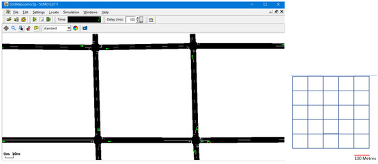
Figure 2.
The SUMO traffic simulator using a 5 × 5 lattice map of 100 m to a side. The screenshots show the simulator UI, while the lattice graphic represents the full layout of the map used by the agents.
Each simulation, except for the first set below, simulates 100 agents using the map simultaneously. Although configuration parameters are changed between simulations, all simulations use the same set of origin and destination locations for the agents. As well, each agent is limited to starting and ending their route at an intersection, rather than in the middle of a road segment. We limit the number of simulations runs to 60 per set of parameters in each scenario, except for the first. This limit is selected as each simulation run represents the same day in repeated weeks. As such, for the routing method to be of value to a driver, it must produce improved routing results over a small number of attempts, leading us to use a limited number of runs for each scenario. The following six sets of simulation scenarios/methods are used:
- (1)
- Each agent simulated individuallyEach agent is provided with the five fastest routes from the modified A* algorithm and allowed to run through each as the sole agent in the simulation. The fastest of the five is then selected as the fastest possible route time for the agent to travel from its origin to its destination without delays due to traffic congestion.
- (2)
- Simulation with direct experience but no re-routingThe simulation is run using 100 agents that are limited to using only the travel time data they can collect directly. The agents start by exploring the five fastest potential routes from the modified A* algorithm to determine the fastest one and then select a route as they gain further experience. The SAW formula is used to estimate the fastest route, but each agent uses an epsilon-greedy algorithm [8] to make their selection, with the epsilon value varied as one of the simulation parameters. The simulations are run 60 times with the SAW weight fixed such that the same weight value is used for all simulations for a given set of parameters.
- (3)
- Simulation with a TIS but no re-routingThe simulation is run using 100 agents that can learn a new SAW weight at varying rates using all travel time data available from the TIS. The SAW formula is used to estimate the fastest routes from a list of potential routes and the agents select the fastest estimate. After each simulation, the agent reviews the actual travel time for each potential route and determines what the SAW weight would need to be for the agent to have selected the fastest route. The simulations are run 60 times for each set of parameters.
- (4)
- Simulation with direct experience and re-routingThe simulation is run using 100 agents that are limited to using only the travel time data they can collect directly. This set of simulations is identical to the simulations in method (2), with the exception that a route performance factor of 1.5 is set for each set of simulations. The performance factor is a setting that allows the agent to calculate a new route from the next intersection they will occupy, to their destination. In the case of these simulations, the agent will only attempt to re-route if the total time they have experienced on a route is greater than 1.5 times the expected route time to that point. While an agent can consider re-routing at each intersection, each agent is only allowed to select a re-route once in each simulation. The simulations are run 60 times for each set of parameters.
- (5)
- Simulation with a TIS and re-routingThe simulation is run using 100 agents that can learn a new SAW weight at varying rates using all travel time data available from the TIS. This set of simulations is identical to simulations in method (3), with the exception that a route performance factor of 1.5 is set for each set of simulations. The simulations are run 60 times for each set of parameters.
- (6)
- Simulation with a combination of a TIS and direct experienceThe simulation is run using 100 agents that are allowed to learn a new SAW weight at varying rates using all travel time data available from the TIS. Re-routing is not allowed for the agents.This set of simulations differs from method (3) in that agents are also able to learn from direct experience. After an agent is provided a list of potential routes with estimated route times from applying the SAW formula, it reviews its previous route experience. If the route with the fastest estimated route time has not been used before, the agent will always select it. If the best estimated route is the same as the route used in the previous simulation, the agent selects the same route again. If the best estimated route is different from the route used in the previous simulation, the agent compares the estimated route time to the actual route time from the previous simulation. The previous route’s travel time is modified by an exploration factor of 0.5. If the estimated route is faster than the adjusted previous route time, the agent selects the new route. The simulations are run 60 times for each set of parameters.
4.3. Experimental Analysis
To measure the effectiveness of routing with a TIS we measure the price of anarchy [30]. The price of anarchy is the social cost due to congestion. In the case of vehicle routing it can be measured as the increase in route times that would not otherwise be experienced if congestion were non-existent. The price of anarchy is calculated as the ratio of the social cost of congestion to the social cost at a minimizing action distribution [30] and the social cost is measured as:
where:
is a set of players of different types.
, where is the set of actions related to a set of resources R. The action is selected by all players of type i. The action represents a segment of the player’s path ;
, where is a cost function for road segment and is nonnegative, continuous and nondecreasing.
is the element of s that corresponds to the set of players of type i who select action .
The price of anarchy is thus:
In our research, the value of is calculated by summing the fastest route time for each agent when no other agents are being simulated. This data are collected using simulation scenario 1. As such, the minimized action distribution represents the fastest route time possible, given the list of origins and destinations being used.
The value of is calculated as the sum of the route times when all agents are simulated simultaneously. The price of anarchy ratio will always give a value greater than or equal to 1, where 1 indicates the agents have found a set of routes that provides the fastest possible route times. The method with the lowest price of anarchy for a given set of parameters at user equilibrium will be considered to provide the fastest routing solutions for all agents.
5. Simulation Results
For all simulation scenarios/methods, except for the first, the following data are presented for each set of parameters:
- The total route time for all agents on the 60th simulation. As this is the final simulation run for a given set of parameters, it represents the point at which the agents will no longer be able to modify their routes.
- The price of anarchy at the 60th simulation.
- The minimum price of anarchy across all simulations.
- The mean price of anarchy. This value is presented to show the difference between the final simulation results and the average for the method.
- The median price of anarchy. This value is presented to show the overall effectiveness of the method across all simulations.
- The number of times user equilibrium was achieved. Equilibrium may last for a single pair of simulations or may be repeated across multiple simulations.
- Where re-routing is used, the minimum number of re-routes across all simulations.
5.1. Each Agent Simulated Individually
The total travel time for all agents using their best route is: 3431.4 s. This number is used as the value when calculating the price of anarchy.
5.2. Simulation with Direct Experience but No Re-Routing
Each set of simulations is run 60 times and has a fixed SAW weight, such that the agent does not change the weight between simulations. The mean and median price of anarchy is calculated using only the 6th through 60th simulations as the agents are still exploring potential routes in the 1st through 5th simulations, which would skew the values. The epsilon values determine the percentage chance that the epsilon-greedy algorithm will select a route other than the fastest provided by the A* algorithm and their previous experience. Thus, an epsilon of 10 represents a 10 percent chance that the agent will select a random alternate route to find a faster route along traffic congested roads.
Minimum and Median Price of Anarchy.Figure 3 displays the minimum and median price of anarchy for each set of parameters. The minimum price of anarchy was lowest when epsilon was set to 5 for all SAW weights, except for w = 0.5, where an epsilon of 15 provided the lowest value. The lowest median occurred where epsilon was 0, regardless of the weight used. That the median price of anarchy was consistently lowest when epsilon is 0, while also being highest at an epsilon of 20, shows us that agents are able to exploit their known routes more effectively when other agents are less likely to explore novel routes. The difference between the minimum and median price of anarchy for each set of routing parameters was found to vary between 0.013 and 0.116, with the largest differences occurring where higher epsilon values were used.
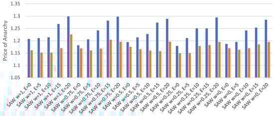
Figure 3.
Minimum/median price of anarchy with direct experience, no re-routing.
User Equilibrium Points.Figure 4 displays the number of occurrences of user equilibrium for each set of parameters. Equilibrium occurred only where the epsilon value was set to 0 as the agents would randomly select alternative routes when using higher epsilon values, regardless of their perceived likelihood of producing a better route time, preventing equilibrium from being achieved.
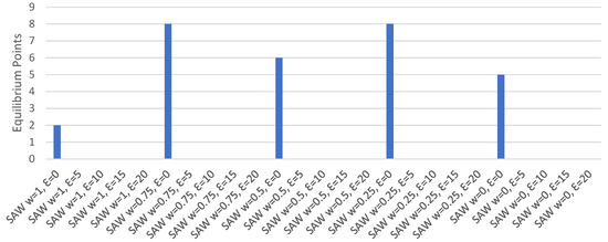
Figure 4.
Equilibrium points with direct experience, no re-routing.
5.3. Simulation with a TIS but No Re-Routing
Each set of simulations is run 60 times. The first five sets of simulations use a fixed SAW weight, the remaining sets allow the agents to change the weight by an amount ranging from 0.1 to 1.0 between each simulation. The mean and median price of anarchy is calculated using only the 6th through 60th simulations as the agents have not yet produced sufficient travel time data to avoid using estimated times in the 1st through 5th simulations. Where travel time data are not available, the agent calculates an estimate using the allowed road speed and road segment length.
Minimum and Median Price of Anarchy.Figure 5 displays the minimum and median price of anarchy for each set of parameters. The minimum price of anarchy was lowest when the agents could change their SAW weights by up to 0.3 between routing episodes. The median price of anarchy was lowest where the agents could change their SAW weights by up to 0.1 between routing episodes. The difference between the lowest median price of anarchy and the highest was 0.027. However, when fixed SAW weights are not included the difference drops to 0.014, indicating that there is greater similarity in the median price of anarchy when the agents are able to change their weight values, regardless of the amount of change allowed. The difference between the minimum and median price of anarchy for each set of routing parameters was found to vary between 0.019 and 0.038. This is a smaller range of differences than was found using direct experience only. As well, the highest median price of anarchy, 1.141, was found be lower than the lowest median value when using direct experience, 1.179.
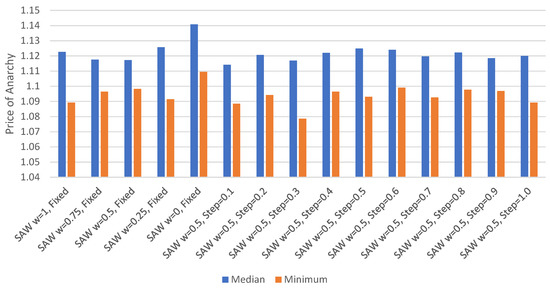
Figure 5.
Minimum/median price of anarchy with TIS, no re-routing.
5.4. Simulation with Direct Experience and Re-Routing
Each set of simulations is run 60 times and has a fixed SAW weight, such that the agent does not change the weight between simulations. The mean and median price of anarchy is calculated using only the 6th through 60th simulations as the agents are still exploring potential routes in the 1st through 5th simulations, which would skew the values. Each agent can re-route a maximum of one time per simulation with a performance factor of 1.5. The re-route decision is made at the end of each road segment by multiplying the estimated route time to the end of the segment by 1.5 and comparing the actual route time to that point. If the actual time is greater than this value and the agent has not re-routed, the agent will re-route.
Minimum and Median Price of Anarchy.Figure 6 displays the minimum and median price of anarchy for each set of parameters. The minimum price of anarchy was lowest when epsilon was set to 5 for all SAW weights, except for w = 0.5, where an epsilon of 0 provided the lowest value. The lowest median occurred where epsilon was 0, regardless of the weight used. As with direct experience with no re-routing, the highest median price of anarchy was found when an epsilon of 20 was used. The highest median value with re-routing, 1.29, is comparable to the highest median with no re-routing, 1.299. However, the lowest median with re-routing, 1.149, is lower than the lowest median with no re-routing, 1.179, suggesting that there is a small benefit to using re-routing. The difference between the minimum and median price of anarchy for each set of routing parameters was found to vary between 0.009 and 0.113. This is comparable to the difference found when no re-routing was used, 0.013 and 0.116, indicating that re-routing had little effect in reducing the gap between the minimum and median.
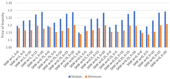
Figure 6.
Minimum/median price of anarchy with direct experience, re-routing.
User Equilibrium Points and Minimum Re-routes.Figure 7 displays the number of occurrences of user equilibrium and minimum re-routes for each set of parameters. Equilibrium occurred only where the epsilon value was set to 0, with the highest number of equilibrium points being 6 for w = 0.5. A comparison to direct experience with no re-routing indicates that the use of re-routing reduces the frequency of equilibrium. The minimum number of re-routes was found to be lowest where the SAW weight was 0 and epsilon was 0, while the trend across all sets of parameters showed that the minimum number of re-routes was highest with larger epsilon values. This is consistent with the equilibrium point data in that lower epsilon values tended to result in fewer poor route selections that would require correction through re-routing.
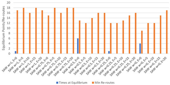
Figure 7.
Equilibrium points and re-routes with direct experience.
5.5. Simulation with a TIS and Re-Routing
Each set of simulations is run 60 times. The first five sets of simulations use a fixed SAW weight, the remaining sets allow the agents to change the weight by an amount ranging from 0.1 to 1.0 between each simulation. Each agent can re-route a maximum of 1 time per simulation with a performance factor of 1.5. The mean and median price of anarchy is calculated using only the 6th through 60th simulations as the agents have not yet produced sufficient travel time data to avoid using estimated times in the 1st through 5th simulations. Where travel time data are not available, the agent calculates an estimate using the allowed road speed and road segment length.
Minimum and Median Price of Anarchy.Figure 8 displays the minimum and median price of anarchy for each set of parameters. The minimum price of anarchy was lowest when the agents could change their SAW weights by up to 0.3 between routing episodes. The median price of anarchy was lowest where the agents could change their SAW weights by up to 0.1 between routing episodes. The difference between the lowest median price of anarchy and the highest was 0.031; however, when fixed SAW weights are not included the difference drops to 0.012, indicating that, as with using a TIS and no re-routing, there is little difference between median price of anarchy when the agents are able to change their weight values. The highest median price of anarchy with re-routing, 1.147, is comparable to that found with no re-routing, 1.141. When fixed weight routes are not considered, the highest median values are almost identical, at 1.129 with re-routing and 1.128 without. These results suggest that there is no advantage to using re-routing when the agents are able to make use of a TIS for travel time data. The difference between the minimum and median price of anarchy for each set of routing parameters was found to vary between 0.019 and 0.04. The highest median price of anarchy using a TIS and re-routing, 1.147, was found to be lower than the lowest median value when using direct experience with re-routing, 1.149.
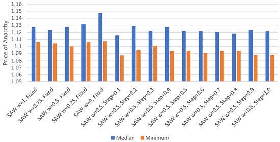
Figure 8.
Minimum/Median Price of Anarchy with TIS, Re-routing.
User Equilibrium Points and Minimum Re-routes.Figure 9 displays the number of occurrences of user equilibrium and re-routing for each set of parameters. No instances of equilibrium occurred. The minimum number of re-routes was found to be lowest where the SAW weight was fixed at 0.25. The highest number of re-routes occurred where the agents could adjust their SAW weight by 0.2 between routing episodes. However, for other simulations where the agents could adjust their weights, the number of minimum re-routes varied from 7 to 8. A comparison of the average minimum number of re-routes shows that direct experience routing used 15, while TIS routing used 8.4, indicating that using a TIS reduced the need to re-route while on route.
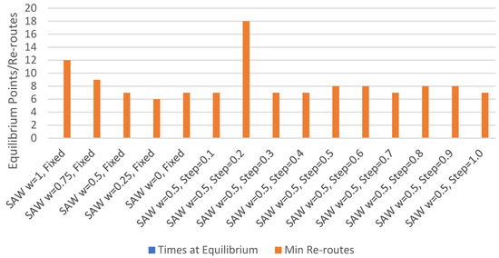
Figure 9.
Equilibrium points and re-routes with TIS.
5.6. Simulation with a Combination of a TIS and Direct Experience
Each set of simulations is run 60 times. The first five sets of simulations use a fixed SAW weight, the remaining sets start with a weight of 0.5 but allow the agents to change the weight by an amount ranging from 0.1 to 1.0 between each simulation. Each agent also uses its direct routing experience to determine whether to select a different route than was used in the previous simulation. The mean and median price of anarchy is calculated using only the 6th through 60th simulations as the agents have not yet produced sufficient travel time data to avoid using estimated times in the 1st through 5th simulations. Where travel time data are not available, the agent calculates an estimate using the allowed road speed and road segment length.
Minimum and Median Price of Anarchy.Figure 10 presents the median and minimum price of anarchy for each set of parameters. The median price of anarchy was found to be lowest where the agents could change their SAW weights by up to 0.9 per routing episode. The lowest minimum price of anarchy was found when the agents could change their SAW weights by up to 1.0 per routing episode. The difference between the minimum and median price of anarchy for each set of routing parameters was found to vary between 0.003 and 0.037. The highest median using a TIS with individual experience, 1.120, was found to be less than the lowest median when using individual experience with re-routing, 1.149, but slightly higher than the lowest median using a TIS with re-routing, at 1.116. The difference between the minimum and median price of anarchy for each set of routing parameters was found to vary between 0.003 and 0.037. This is a smaller variation than that found for direct experience with re-routing, 0.009 to 0.113, but larger than when using a TIS with re-routing, 0.019 to 0.04.
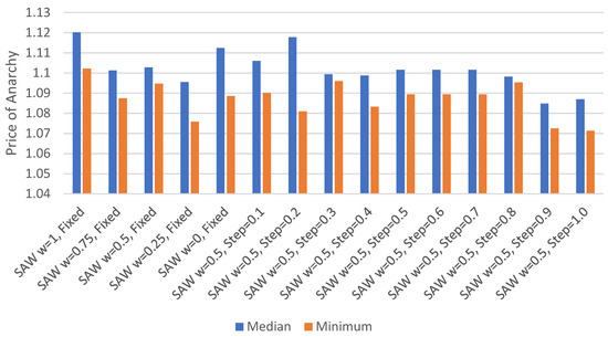
Figure 10.
Minimum/median price of anarchy with TIS and direct experience.
User Equilibrium Points.Figure 11 presents the number of occurrences of user for each set of parameters. Equilibrium occurred with all sets of parameters but was highest where the SAW weight was fixed, and weight was not equal to 0. This method was the only one found to have reached equilibrium regardless of the parameters used.
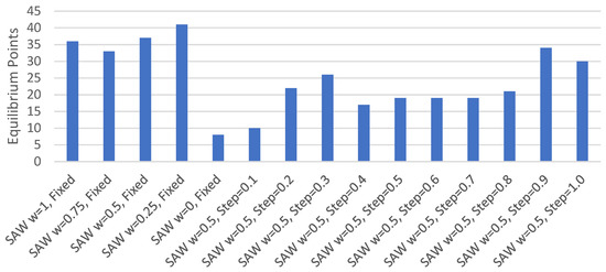
Figure 11.
Equilibrium points with TIS and direct experience.
6. Discussion
Table 1 presents the price of anarchy and total travel time data for the set of simulation parameters that produced the lowest median price of anarchy for each of our routing methods. Figure 12 and Figure 13 display the simulation results for each of the parameter sets in Table 1.

Table 1.
Parameters by method with lowest median Price of Anarchy (POA), results.
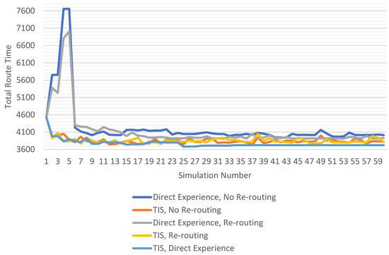
Figure 12.
Total route time by bethod using best parameters.
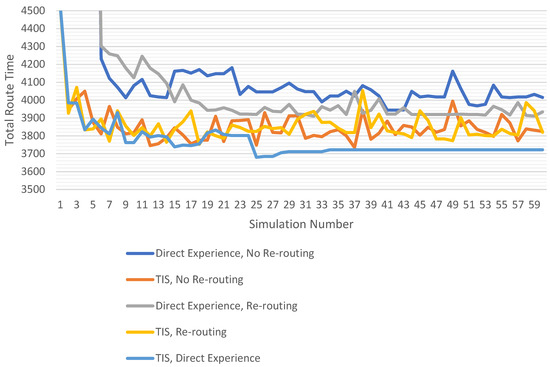
Figure 13.
Total route time by method using best parameters—enlarged.
6.1. Revisiting the Research Objectives
Now let us discuss our results as they pertain to our research objectives. For Objective 1, determining the fastest route for the driver with the least exploration, we note that all routing methods produced an initial simulation with a total route time of 4524.8 s. This is due to each method using the same modified A* algorithm to build each agent’s list of potential routes. As the algorithm relies upon map data alone, it always provides the same fastest route, and as the agents have no initial travel time data beyond that provided by the map, they always select the same route. Once the agents have completed their first simulation the methods diverge. Figure 12 shows that the both the TIS and TIS with direct experience methods were able to quickly reduce their total route times from the initial simulation, while the methods that rely on direct experience alone see a large increase in route times before dropping in the 6th simulation. This increase in route times is due to the agents’ need to explore alternative routes to develop an initial set of travel time data to apply to the potential route list. Once the agents have completed their initial exploration, they use the travel time data collected to develop routes that improve upon the total route time found in the initial simulation. For the cost of exploration, the agents must try potentially worse routes to determine which is better with congestion. This shows us a drawback to relying on direct experience alone. If the agent must rely on their own experiences to determine which route is most likely to be the fastest on congested roads, then they will always see poorer routing results while acquiring this experience. We also see that as the TIS methods use the collective travel time data of all agents, each agent can avoid this period of exploration and see routing improvements immediately.
For research Objective 2, the routing method must adapt to changes in congestion over successive routing actions, each of the routing methods showed adaptation to changes in congestion. When using direct experience alone, with fixed SAW weights, the agents were able to produce a lower median price of anarchy when using a lower weight value. As well, Figure 3 and Figure 6 show that, with or without re-routing, a weight value of 1.0 resulted in the highest median price of anarchy. The poorer performance when using a high SAW weight is due to the agent’s reliance upon long-term travel time data, which would be used exclusively when the weight is set to 1.0. As the long-term travel times used by the agents are averages from all previous simulations, the agent is less able to adapt to recent changes in congestion that comprise a relatively small component of this value. When combined with the agent’s limited ability to gather travel time data, this results in slower route times. Connecting the agents to a TIS produced greater adaptability to changes in congestion. As each agent had access to the travel time data produced by all other agents, they were able to select the route that was predicted to give the fastest route time, regardless of whether they had used it previously. Under these conditions, the agents were found to produce the lowest median price of anarchy where the SAW weight was not fixed. During simulation, many agents were observed to change their weight values between routing episodes, often by as much as they could by the step limit; however, some agents rarely changed their SAW weights. This shows us that it is better for the agents to be able to modify their weight value to adapt to changes in the congestion problem. Finally, when the agents were able to combine both a TIS and direct experience, they were best able to adapt to changes in congestion. This is reflected in this method having the lowest median price of anarchy. The use of direct experience prevents the agents from chasing the fastest route without regard for past results, allowing the congestion on each road segment to stabilize and become more predictable.
For research Objective 3, the routing method must produce routes that are fair for each driver but also minimizes the total travel time for all drivers, the multi-agent routing methods produced routes that were fair to the drivers, as each agent had the goal of selecting the fastest route to reach their destination. However, while each method proved successful at reducing the median price of anarchy and the price of anarchy on the 60th simulation, the combined TIS with direct experience method showed the lowest values. Figure 13 shows that the TIS with direct experience method provided a total route time on the 60th simulation that was 100 s lower than when using a TIS alone, and 212 s lower than direct experience with re-routing. As well, user equilibrium was maintained from the 34th simulation, demonstrating that all agents had found the fastest route possible, given the existing congestion.
6.2. User Equilibrium
Further, from the simulation, user equilibrium was found to occur where the agents used direct experience alone, with or without re-routing, and where the agents used a combination of a TIS with direct experience. User equilibrium was not observed where only the TIS was used. Figure 4 and Figure 7 show that where direct experience alone was used, the agents reached equilibrium more often when they were unable to re-route. This was because of re-routing on the congestion problem. Where many agents re-route, the congestion on any given road segment may change from routing episode to routing episode. As the congestion changes, the agents adapt their paths to produce better route times, resulting in fewer instances of user equilibrium. The number of agents changing routes in consecutive simulations ranged between 10 to 20 percent, regardless of whether re-routing was. This is due to the agents adjusting their paths to select the fastest route given the existing congestion pattern. As the agents are not including their direct experiences routing—relying only on the collective experience of the TIS—they select the fastest route recommended by their application of the SAW formula. While many agents change their routes, the congestion pattern changes, thus the agents never reach a point of user equilibrium. It should be noted, however, that most agents will use the same route in consecutive routing episodes.
User equilibrium was found to occur most often when using a combination of TIS and direct experience. Figure 11 shows that user equilibrium occurred for all parameter sets and many more times than when direct experience alone was used. This was due to the agents use of past routing experiences to guide their selection of future routes. As the agents only selected routes that had been shown to be fast in the past, they were less likely to change routes between routing episodes. As such, once a fast route was found, the agents stayed with it, resulting in more instances of user equilibrium. The earliest point of equilibrium was found to occur by the 10th simulation for most sets of parameters, although this was not held for more than two consecutive simulations. The agents in Figure 13 reached a point of consistent equilibrium by the 26th simulation, however, the equilibrium point does change at the 28th and 34th simulations, where some agents adjust their routes. As using a TIS with direct experience produces user equilibrium points that last across many simulations, and does so earlier than direct experience alone, we can say that this method does achieve user equilibrium with fewer routing episodes than either of our other methods.
6.3. Re-Routing Effectiveness
Re-routing while on route lowered total route times for agents using direct experience alone but had little effect when using a TIS. When agents had no access to a TIS, the ability to re-route allowed the agents to correct for a poor routing decision given the congestion encountered on its route. This is reflected in a lower median price of anarchy when re-routing is used. Using a TIS removed the advantage given by re-routing, as the agents are relying upon travel time data provided by all agents and are able to make better routing choices. The difference between the two methods shows that there is no advantage to using re-routing where a TIS is available; however, in instances where the TIS becomes unavailable—for example, in the case of a communications failure—the ability to re-route would be beneficial to the agents.
6.4. Weighting Factor
When simulation parameters were set to allow the agents to adjust their SAW weights, it was found that many agents did not reach an equilibrium point and continued to make changes to their weighting factor. This was observed as the agents were making changes to their routes and at user equilibrium.
6.4.1. Localization of the SAW Weight
The ideal SAW weight is localized to the road segment to which it is applied. Over many simulations, congestion on a road segment may change, depending on the routing decisions of the agents using it. As changes in congestion on one road segment may be different than on another segment, the weighting factor that produces the most accurate estimate of the time to travel any given segment may be different than for another segment.
As the SAW weight used by an agent represents an aggregation of the weight for each road segment on a route, the ideal weight for an agent depends on the route used. When building a route, there is often little difference between fastest paths for the agent—the geography of the map is such that these routes may vary by only a few road segments. Thus, as the agent is learning which weighting factor is best, they will find a value that may differ significantly from the weighting factor used by an agent that is routing in a different part of the city. As such, while there were agents that were observed having the same weighting factor, often many agents used weights that were unique to their origin and destination.
6.4.2. Changes in Weighting Factor at User Equilibrium
Many agents were found to change their weighting factor when at user equilibrium. Often the changes were the largest allowed by the SAW weight step limit, such that an agent might select a weight of 0 in one simulation and then a weight of 1 in the next. When using a TIS with direct experience the agents will only select a route that is different than that used in the previous routing episode if the route is new to the agent or is significantly faster than route they used previously. As displayed in Figure 13, this eventually allows the agents to reach a user equilibrium. It also has the effect of stabilizing the congestion problem, as the agents always use the same road segments in the same order.
The stability of the congestion problem affects the travel time data provided to the agents. As the agents use a combination of short-term and long-term travel time averages to calculate their weighting factor, the longer congestion remains consistent, the more similar the short-term and long-term averages become. This results in there being little difference in estimated route times, regardless of the SAW weight used, and the agent makes changes to the weight value based on smaller differences between the two averages.
As such, we see that stabilization of the congestion problem is more important than selecting the most appropriate SAW weight when an agent is attempting to select the fastest route to their destination. We found that the combination of a TIS and direct agent experience allowed our agents to achieve a total route time that is significantly lower than when using either a TIS or direct experience alone. The combined system produced a lower median price of anarchy than either of the other methods, with or without re-routing, while also having a lower price of anarchy on the 60th simulation.
7. Conclusions and Future Work
We have studied formulated and simulated vehicle routing strategies to reduce travel times in a traffic congested city. Through multi-agent simulation, we compared five routing methods: (1). Developing routes using only travel time data an agent could collect through direct experience. (2). Using a centralized real-time traffic information system (TIS) to provide travel time data provided by all agents. (3). Routing with direct experience alone but allowing the agents to re-route while on route. (4). Relying on a TIS for travel time data while also using re-routing while on route. (5). Combining travel time data from a TIS with previous routing experience. We ran experiments in which we simulated vehicles traveling in a city road network grid, each directed by an agent. We found that each method reduced the total route times of all agents when compared to routing by selecting the fastest route based on map data alone. However, using a TIS provided further reduced route times over that found when using direct experience alone. We also found that re-routing improved results when using direct experience but not when using a TIS, as the agents were able to better predict the effects of congestion on their routes. More importantly, we found that the combination of a TIS with direct routing experience provided the lowest total route time of all methods tested, while also maintaining user equilibrium for longer periods than when using direct experience alone. As such, we have concluded that the combined routing method would provide the most benefit for drivers navigating in a congested city.
The large amount of travel time data that the TIS makes available requires the agents to have a means of finding data that is useful in making a routing decision. The use of averaged travel times and the SAW formula allow the agents to do this; however, this method is not the only way we can make use of this data. Further research is necessary to determine which data analysis techniques may be performed on the data in the TIS to find patterns or trends in the traffic congestion problem. As well, additional study of the agents may produce alternative algorithms to estimate their route times, possibly leading to different route selections and a user equilibrium with a lower total route time. Further, as the agents make decisions based partly upon the travel time data, they receive from the TIS, there is an opportunity to affect their decisions by making modifications to the travel times provided to them. If we consider that sending an arbitrarily large travel time to an agent would effectively cause them to avoid a route using the affected road segment, we see a few potentially useful possibilities. In the case of road closure due to an accident, temporarily increasing the travel time along the road would cause agents to route around the affected area. This technique may also be useful in reducing the number of vehicles that attempt to use a road that is under construction. As well, in the case of evacuations, vehicles could be encouraged to use some roads but not others by modifying the travel times provided. While modifying travel times could be useful in managing the flow of vehicles, further research is required to determine how the desired results could be achieved without unanticipated consequences that may make an existing problem worse.
Author Contributions
Conceptualization, methodology, validation, formal analysis, writing—original draft preparation, review and editing, visualization, A.S., F.L. and D.W.; software, resources, A.S. and F.L.; data curation, experimental investigation, A.S; writing—review, X.Z.; supervision, F.L. and D.W.; project administration, A.S. and F.L.; funding acquisition, F.L. All authors have read and agreed to the published version of the manuscript.
Funding
This research received no external funding and the APC was funded by NSERC DG.
Data Availability Statement
Not Applicable.
Acknowledgments
We acknowledge the support of the Natural Sciences and Engineering Research Council of Canada (NSERC).
Conflicts of Interest
The authors declare no conflict of interest.
References
- Mandayam, C.V.; Prabhakar, B. Traffic congestion: Models, costs and optimal transport. ACM Sigmetrics Perform. Eval. Rev. 2014, 42, 553–554. [Google Scholar] [CrossRef]
- Bazzan, A.L.; Chira, C. A Hybrid Evolutionary and Multiagent Reinforcement Learning Approach to Accelerate the Computation of Traffic Assignment. In Proceedings of the 2015 International Conference on Autonomous Agents and Multiagent Systems, Singapore, 4–8 May 2015; pp. 1723–1724. [Google Scholar]
- Hardin, G. The tragedy of the commons. Science 1968, 162, 1243–1248. [Google Scholar] [CrossRef] [PubMed]
- Dijkstra, E.W. A note on two problems in connexion with graphs. Numer. Math. 1959, 1, 269–271. [Google Scholar] [CrossRef]
- Hart, P.E.; Nilsson, N.J.; Raphael, B. A formal basis for the heuristic determination of minimum cost paths. IEEE Trans. Syst. Sci. Cybern. 1968, 4, 100–107. [Google Scholar] [CrossRef]
- Thathachar, M.; Sastry, P.S. A new approach to the design of reinforcement schemes for learning automata. IEEE Trans. Syst. Man, Cybern. 1985, 1, 168–175. [Google Scholar] [CrossRef]
- Auer, P.; Cesa-Bianchi, N.; Fischer, P. Finite-time analysis of the multiarmed bandit problem. Mach. Learn. 2002, 47, 235–256. [Google Scholar] [CrossRef]
- Sutton, R.S.; Barto, A.G. Multi-armed Bandits. In Reinforcement Learning: An Introduction, 2nd ed.; The MIT Press: Cambridge, MA, USA, 2018; Chapter 2; pp. 25–46. [Google Scholar]
- Google. Google Traffic. Available online: https://www.google.ca/maps/ (accessed on 10 August 2021).
- Waze Mobile. Waze. Available online: https://www.waze.com/ (accessed on 10 August 2021).
- Roughgarden, T. Stackelberg scheduling strategies. SIAM J. Comput. 2004, 33, 332–350. [Google Scholar] [CrossRef]
- Desjardins, C.; Laumônier, J.; Chaib-draa, B. Learning agents for collaborative driving. In Multi-Agent Systems for Traffic and Transportation Engineering; IGI Global: Hershey, PA, USA, 2009; pp. 240–260. [Google Scholar]
- Bazzan, A.L. Opportunities for multiagent systems and multiagent reinforcement learning in traffic control. Auton. Agents Multi-Agent Syst. 2009, 18, 342. [Google Scholar] [CrossRef]
- Wang, S.; Djahel, S.; Zhang, Z.; McManis, J. Next road rerouting: A multiagent system for mitigating unexpected urban traffic congestion. IEEE Trans. Intell. Transp. Syst. 2016, 17, 2888–2899. [Google Scholar] [CrossRef]
- Horng, G.J.; Cheng, S.T. Using intelligent vehicle infrastructure integration for reducing congestion in smart city. Wirel. Pers. Commun. 2016, 91, 861–883. [Google Scholar] [CrossRef]
- de Oliveira, D.; Bazzan, A.L. Multiagent learning on traffic lights control: Effects of using shared information. In Multi-Agent Systems for Traffic and Transportation Engineering; IGI Global: Hershey, PA, USA, 2009; pp. 307–321. [Google Scholar]
- Wardrop, J. Some theoretical aspects of road traffic research. Proc. Inst. Civ. Eng. 1982, 1, 325–378. [Google Scholar] [CrossRef]
- Levy, N.; Klein, I.; Ben-Elia, E. Emergence of cooperation and a fair system optimum in road networks: A game-theoretic and agent-based modelling approach. Res. Transp. Econ. 2018, 68, 46–55. [Google Scholar] [CrossRef]
- Tumer, K.; Proper, S. Coordinating actions in congestion games: Impact of top–down and bottom–up utilities. Auton. Agents Multi-Agent Syst. 2013, 27, 419–443. [Google Scholar] [CrossRef]
- Shoham, Y.; Leyton-Brown, K. Congestion Games. In Multiagent Systems: Algorithmic, Game-Theoretic, and Logical Foundations; Cambridge University Press: Cambridge, MA, USA, 2009; Section 6.4; pp. 201–213. [Google Scholar]
- Shoham, Y.; Leyton-Brown, K. Teams of Selfish Agents: An Introduction to Coalitional Game Theory. In Multiagent Systems: Algorithmic, Game-Theoretic, and Logical Foundations; Cambridge University Press: Cambridge, MA, USA, 2009; Chapter 12; pp. 383–408. [Google Scholar]
- Yamashita, T.; Izumi, K.; Kurumatani, K.; Nakashima, H. Smooth traffic flow with a cooperative car navigation system. In Proceedings of the Fourth International Joint Conference on Autonomous Agents and Multiagent Systems, Utrecht, The Netherlands, 25–29 July 2005; pp. 478–485. [Google Scholar]
- Levy, N.; Ben-Elia, E. Emergence of system optimum: A fair and altruistic agent-based route-choice model. Procedia Comput. Sci. 2016, 83, 928–933. [Google Scholar] [CrossRef][Green Version]
- Erev, I.; Ert, E.; Roth, A.E. A choice prediction competition for market entry games: An introduction. Games 2010, 1, 117–136. [Google Scholar] [CrossRef]
- Lattimore, T.; Szepesvári, C. Bandit Algorithms; Cambridge University Press: Cambridge, MA, USA, 2020. [Google Scholar] [CrossRef]
- Zhou, J.; Lai, X.; Chow, J.Y.J. Multi-armed bandit on-time arrival algorithms for sequential reliable route selection under uncertainty. Transp. Res. Rec. 2019, 2673, 673–682. [Google Scholar] [CrossRef]
- Yoon, G.; Chow, J.Y.J. Contextual bandit-based sequential transit route design under demand uncertainty. Transp. Res. Rec. 2020, 2674, 613–625. [Google Scholar] [CrossRef]
- Sutton, R.S.; Barto, A.G. Upper-Confidence-Bound Action Selection. In Reinforcement Learning: An Introduction, 2nd ed.; The MIT Press: Cambridge, MA, USA, 2018; Section 2.7; pp. 35–36. [Google Scholar]
- DLR – Institute of Transportation Systems. SUMO. Available online: http://www.dlr.de/ts/en/desktopdefault.aspx/tabid-9883/16931read-41000/ (accessed on 10 August 2021).
- Shoham, Y.; Leyton-Brown, K. Selfish routing and the price of anarchy. In Multiagent Systems: Algorithmic, Game-Theoretic, and Logical Foundations; Cambridge University Press: Cambridge, MA, USA, 2009; Section 6.4.5; pp. 180–181. [Google Scholar]
Publisher’s Note: MDPI stays neutral with regard to jurisdictional claims in published maps and institutional affiliations. |
© 2021 by the authors. Licensee MDPI, Basel, Switzerland. This article is an open access article distributed under the terms and conditions of the Creative Commons Attribution (CC BY) license (https://creativecommons.org/licenses/by/4.0/).