3.1. Cloud State Controller
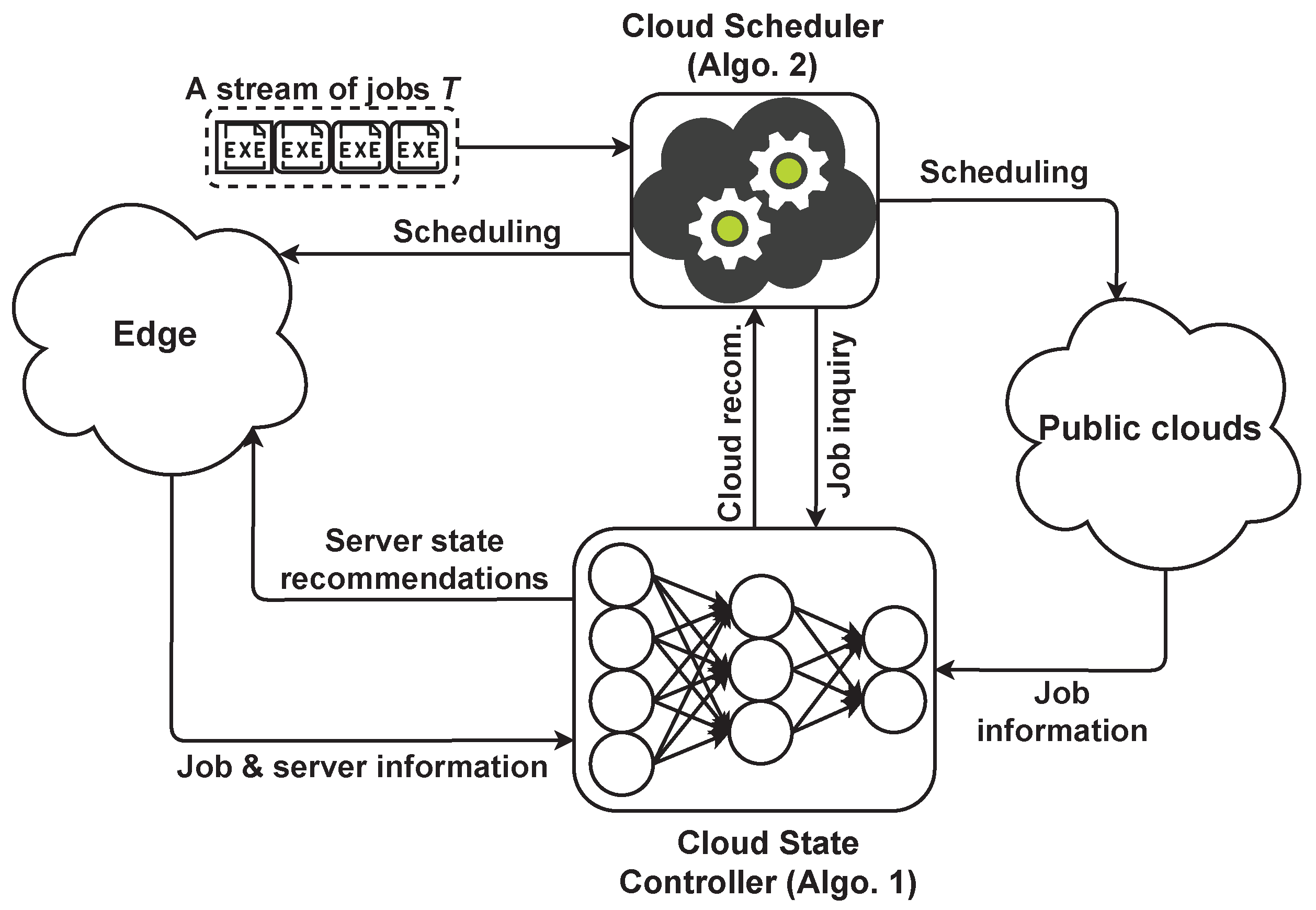
Cloud state controller leverages ANNs for runtime estimation, as well as recommendations to be used for server management in the edge and the job cloud/edge recommendation.
ANNs are computing systems in which examples (i.e., job information or server utilization) are learnt for performing operations, e.g., in terms of cloud environment recommendation or server management. Each neural network consists of connected neurons placed in network layers, and transformations are applied to the value of neurons. Transformations are done by non-linear activation functions to output a value for transmission to the next layer through the network edges. Thus, each value goes through consecutive network layers, starting from an input layer, one layer, or multiple hidden layers and terminating at the output layer. Neurons and edges in a neural network are assigned weights that are adjusted during the network training.
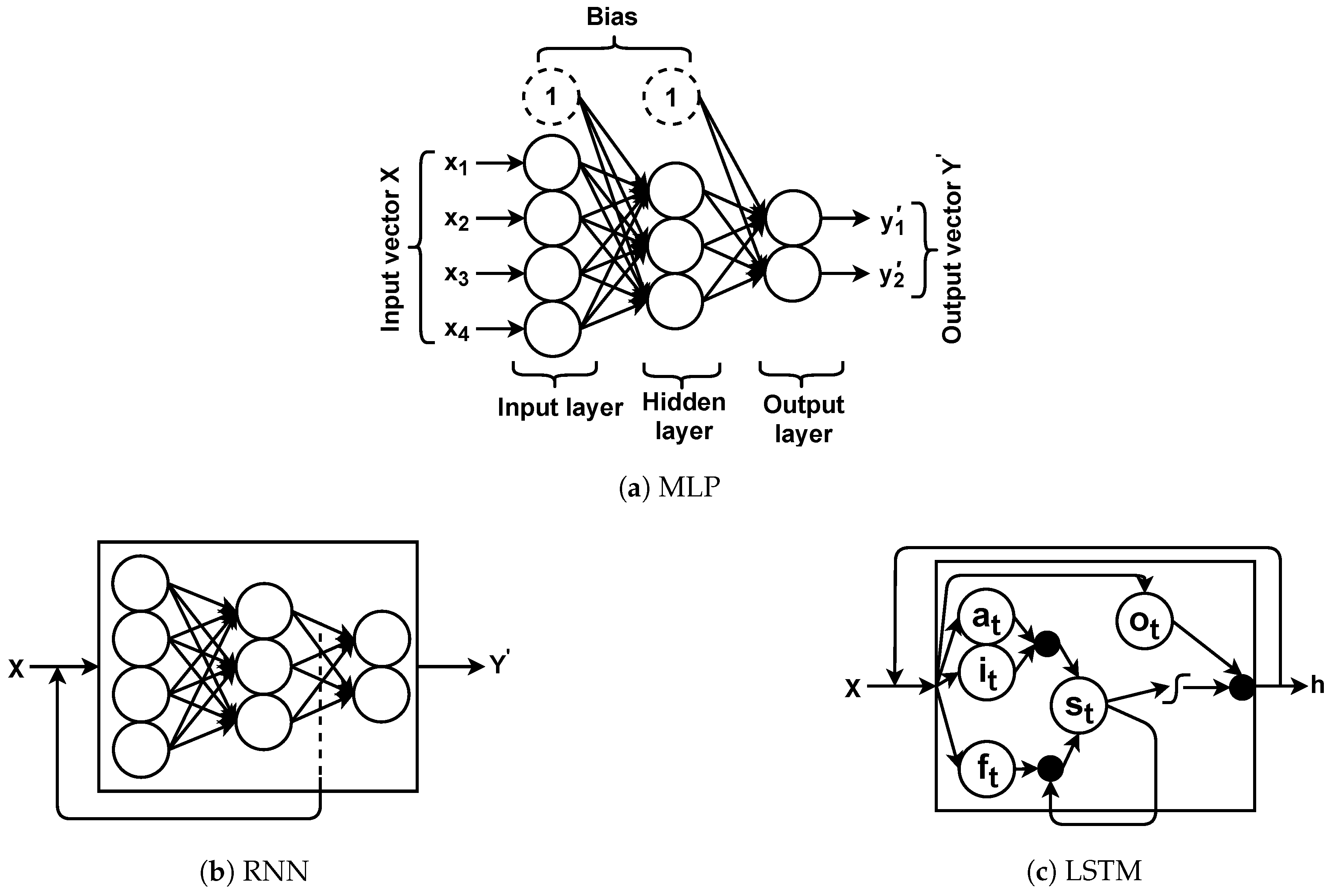
Neural networks used in this study are in different forms referred to as MLP, RNN, or LSTM [
29], which are shown in
Figure 3.
The MLP is a feed-forward neural network that is trained per each input vector in a supervised manner by backpropagation algorithm with respect to the actual outputs or labels (i.e., ). The MLP repeats the process (e.g., classification) for new inputs, and weights are adjusted accordingly. RNN is a special form of MLP that any learnt (i.e., the hidden layer weights) information is kept and is passed to the next input. In fact, RNNs are a chain of MLPs that leverage shared weights for training. This is to ensure that any prediction/estimation is outputted based on the seen input information.
Although promising, during the learning process, less past/seen information contributes to the training (i.e., weight adjustments) and it is known as a vanishing gradient. This drawback is addressed by LSTMs as the special form of RNNs comprised of gates to control information flow in the learning process. They also have a chain structure consisting of cells, each of which has four gates; forget gate, input gate, input activation gate, and output gate. The information that should be ignored from a cell is dealt with by the forget gate (). To decide what information should be stored in the cell state, there are two gates called input () and input activation () gates that contribute to the cell state. Finally, it is required to decide what information should be outputted, which is handled by the output gate ().
A neural network receives an input vector (i.e.,
) and outputs an estimated (or interchangeably predicted) output vector (i.e.,
) which can be written as
. Neurons in the neural network layers are assigned weights
that contribute to the neuron output (
) and are interpreted as the weight from
neuron in the
layer to the
neuron in the
layer. Moreover, there are extra neurons called bias that hold a value equal to 1 and are connected to the neurons for shifting the activation function output. Hence, a neuron output (
) based on sigmoid (
) (or tangent hyperbolic (
) or softmax) activation function is defined as follows.
To adjust the neural network weights in ANNs, the actual output vector (
Y) is compared with the predicted output (
) to compute the error (or loss), e.g., mean squared error (MSE). It computes the difference between the
N real outputs and the predicted outputs for weight adjustments calculated as follows.
Without loss of generality, if the neural network weight is
W, the weight adjustment with respect to the computed error (
E) is defined as follows.
In Equation (
13),
∇ is the vector differential operator and
is the learning variable that controls the weight adjustment. The weight adjustment process takes place by the usage of the backpropagation algorithm that performs repetitive procedures in two separate phases; forward pass (
) and backward pass (
). In the former, the input data is fed into the network to produce the predicted results with respect to Equation (
11). In the latter, the error is calculated in Equation (
12) and is propagated back to the neural network to update the network weights.
Considering the ANNs background stated in this section, the RNN is used to control server energy consumption in the edge by autonomously and periodically observing the server utilization. Servers within the edge may be deactivated or activated by a recommended signal. When the signal implies deactivation, a server puts it in deep sleep mode and is added to the idle server list (). Otherwise, it activates a server from the idle list and is added to the active server list (). Controlling active servers () for reducing energy consumption in the edge requires cluster utilization (i.e., CPU and memory) at and till time . This criterion fits in the RNN definition which considers that past seen information for recommendations. Therefore, the RNN is used for the edge server management per specific time intervals to send a signal for activation () or deactivation (), in the case of putting servers in a deep sleep mode to reduce energy consumption.
LSTM uses collected information of jobs in the edge-cloud environment for cloud/edge recommendations. The information is job characteristics and resource requirements that autonomously and per specified interval is logged due to the unknown job finish time. LSTM models univariate time series recommendation problems in which single series of observations exist (i.e., the job specifications including the executed edge/cloud environment) with respect to the past observations of jobs to recommend the next value in the sequence. Moreover, compared to the server management, additional information is available for cloud/edge recommendations that necessitates the usage of a sophisticated ANN (i.e., LSTM) for dealing with learning. Although RNN and LSTM rely on the historical context of input, LSTM provides a modulated output controlled by gates facilitating when to learn or forget, and mitigates the downsides of RNNs.
Finally, the job runtime estimation belongs to a coarse-grained classification problem, meaning that the runtime is classified into a time slot class (
Section 2.2). Formally, for a job
, the classification is interpreted as the time slot
with respect to Equation (
7). This classification is controlled by the MLP neural network that uses the collected information about executed jobs across the edge-cloud environment, which are kept as profiles. Moreover, in the absence of a job runtime, the job cloud recommendations will not be reliable. This is due to runtime estimations to tailor the scheduling decision that uncertainty about the job runtime could blindly lead to an inefficient resource assignment and would affect the quality of scheduling and the cost [
13,
14].
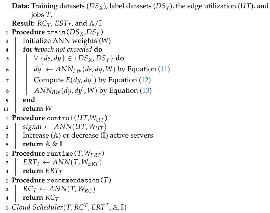
Algorithm 1 presents an overview of the cloud state controller algorithm. This algorithm consists of procedures with respect to recommendation and runtime estimation, and they interact with the train procedure to obtain the corresponding weights for recommendation purposes.
The train procedure takes input datasets (i.e., the server utilization information and job specifications) and separately trains the corresponding ANN under a specified epoch (lines 1–11). The next procedure controls the edge servers with respect to the given utilization, followed by runtime estimation and recommendation procedures. The algorithm returns the estimated runtime, recommended cloud/edge, and active/idle edge server list.
| Algorithm 1: Cloud State Controller (CSC). |
![Information 12 00224 i001 Information 12 00224 i001]() |
3.2. Cloud Scheduler
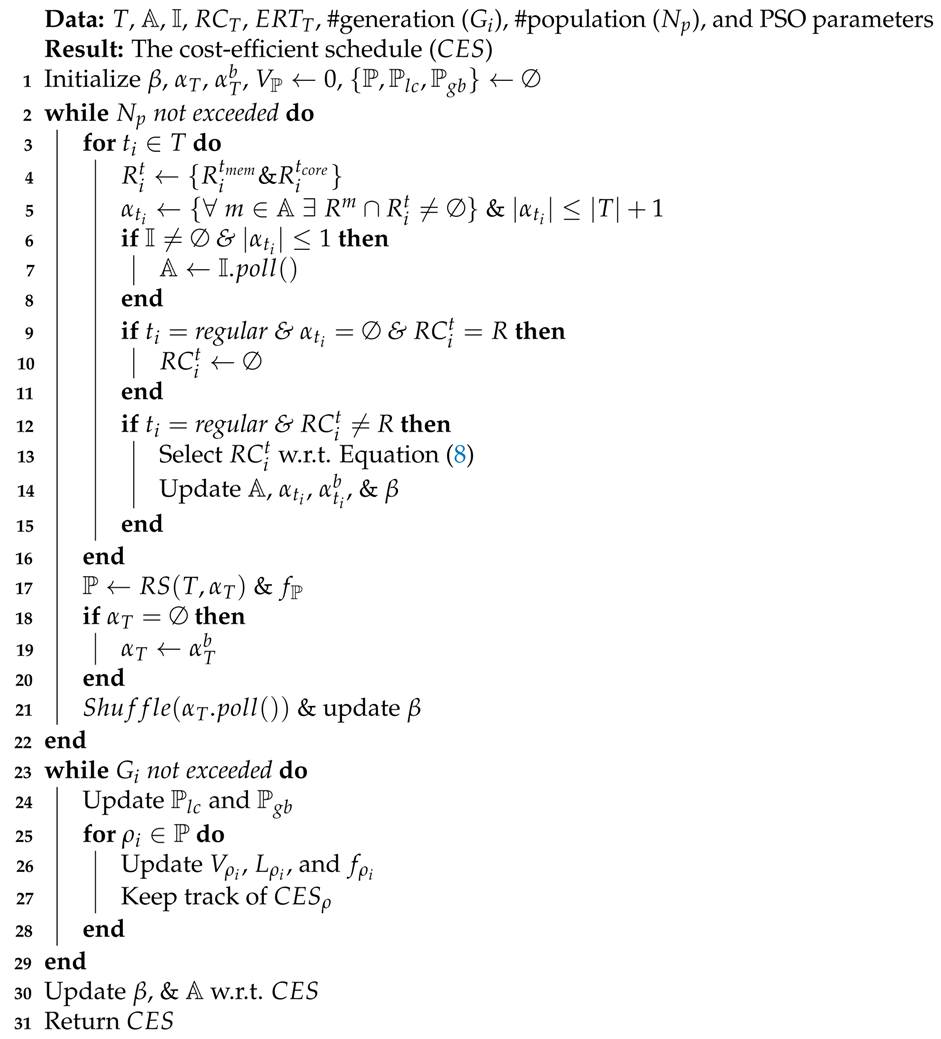
In this section, we explain how the Cloud Scheduler component (Algorithm 2), which was shown in
Figure 1, deals with workload scheduling. The cloud scheduler is a dual-function algorithm that considers runtime estimations for scheduling and may follow recommendations for workload scheduling across the edge-cloud environment.
The cloud scheduler (Algorithm 2) relies on Equation (
8) in the absence of cloud recommendations to heuristically examine which environment—the edge or public clouds—would be cost efficient for scheduling. This algorithm illustrates the workload scheduling across the edge-cloud environment which relies on a particle swarm optimization (PSO)-based algorithm for the edge. The algorithm takes into account runtime estimation or cloud/edge recommendations for scheduling decisions. Scheduling in the edge takes place when a job is privacy-sensitive or it is cost efficient to execute regular jobs with respect to active/idle servers states in the edge. Otherwise, these jobs are offloaded to the cost-efficient public cloud.
| Algorithm 2: Cloud Scheduler (CS). |
![Information 12 00224 i002 Information 12 00224 i002]() |
Meta-heuristic algorithms such as PSO in this study are considered to deal with many complex scheduling problems, such as task scheduling. However they do not guarantee to find optimal solutions—they can be “effective”. The particle swarm optimization algorithm through repetition improves the quality of a candidate solution known as particles (). It aims to move these particles around in the search space based on the position () and the velocity of particles (). Each particle’s movement is affected by the local () and the global () best-known positions toward the best-known positions in the search space (i.e., the population ()). It eventually leads to moving the population (i.e., swarm) toward the best solutions.
A particle structure in the algorithm that is shown in
Figure 4 has a dynamic length equal to the number of available jobs at time
, and each job is assigned to either an edge server (
) or a public cloud virtual machine (
). This selection relies on a candidate list (
) per each job resource requirement (
).
The initial population () is begun with an eligible permutation of job resource selection. There is a list () that maintains resource availability across the edge-cloud environment. Each job in the workload (T) is checked for preparing a list of servers and/or virtual machines that can host a job. The list relies on the edge utilization level in which edge servers are descendingly sorted based on the utilization level (both CPU and memory) at time . The list of each job is capped at servers to avoid computation overhead caused by PSO. Moreover, a job candidate list is updated by adding a temporarily idle server from the list of the edge. This added server would be confirmed if current active servers could not satisfy a job’s resource requirement. Moreover, if a job is privacy-sensitive, it has to choose the edge servers. Otherwise, both edge servers and public cloud virtual machines are taken into account.
When CECBS-R works as the scheduler, Algorithm 2 considers estimated runtimes to assist the selection of cost-efficient resources. Otherwise, it will seek feasible recommendations to schedule jobs onto resources in the edge-cloud environment. In other words, if a regular job is recommended to be scheduled onto the edge with no available servers, the recommended cloud is updated based on the most cost-efficient resources with respect to Equation (
8) that considers billing cycles, and the estimated runtime (
) across the edge-cloud environment.
Per each resource candidate list of a job (), the population is updated by mapping a selected resource to a job for forming a solution. Each solution is evaluated against a fitness function for cost-efficiency and the quality of resource assignment. When a job () is assigned to a candidate resource (m or ), its resource candidate list () and the resource availability list () are updated. If during the process, becomes empty, the backup candidate list () will update the list.
The quality of each particle () is assessed by the fitness function () that consists of controlling and quality parameters, each of which evaluates a particular aspect of the particle. Controlling parameters are defined as the cloud priority () and the job resource allocation ().
A particle may have jobs that are assigned to public cloud virtual machines, however, there should be a mechanism to prioritize edge resource selection. In other words, jobs should be avoided to be processed on the public clouds while the edge has sufficient resources available. Hence,
checks jobs in the particle and penalizes the fitness with
, in which the edge has lower penalized value compared to public clouds, i.e.,
.
Moreover, jobs in a particle should be checked, whether or not the chosen server (m) or the virtual machine () can satisfy jobs resource requirements (). It is expressed as that returns or if the resource requirement is satisfied or not, respectively.
The quality parameters should control the edge utilization (
) and the estimated cost (
). If jobs are assigned to servers in the edge, it should have to increase the overall utilization. Therefore, a particle (
) is assessed against how chosen servers (
) can contribute toward better utilization.
Finally, the estimated cost of a particle (
) for cost-efficiency is computed in Equation (
16). The cost is divided into two parts; the edge and public clouds. The former cost is directly affected by the impact of utilization level on the energy consumption as the higher utilization leads towards the higher energy consumption, and consequently, the higher fitness ratio. In contrast, the latter has a reverse impact on the fitness function, since it aims to reduce the reliance on public cloud resources.
If a server of the edge is assigned to a job (), will consider the electricity cost based on the utilization that the server will have. Otherwise, it will compute the usage cost of virtual machines in public clouds based on the billing cycle.
The fitness function based on the controlling and quality parameters is defined as follows.
In the fitness function, if the denominator is increased, the fitness function will lead toward particles that are not cost efficient. This is due to leaving the edge resources under-utilized and relying more on public clouds. If the numerator is increased and becomes aligned with a small denominator, the fitness function will lead to expressing solutions that are cost efficient and will improve the edge resource utilization.
The PSO algorithm through each iteration updates the best local (
) and global (
) known positions. These positions are the chosen resource indexes in the corresponding candidate list (
) shown in
Figure 5. In order to generate new solutions based on the current population, particles should have to move in the search space with respect to the swarm movement terminology. The movement is controlled by a particle location (
) and its speed (
). Each particle updates its location (
) and its velocity (
) with respect to the
and
, stated in Equations (
18) and (
19), respectively. The velocity of a particle (
) is also controlled by the PSO learning parameters referred to as
,
, and
[
30].
Velocities in the cloud scheduler (Algorithm 2) are the candidate index positions in
for job
. Hence, locations are bounded in the length of
that is updated per new index position provided by the new velocity.
Equation (
20) shows that when the updated velocity (
) in
exceeds the length of
, it will return the reminder as the new index for choosing a new candidate.
Figure 5 illustrates that if the current index for job
in
is 2, the updated velocity
} (
) will change the location.
