
Exploring the Value of Nodes with Multicommunity Membership for Classification with Graph Convolutional Neural Networks


Abstract
1. Introduction
2. Methodology
2.1. Data
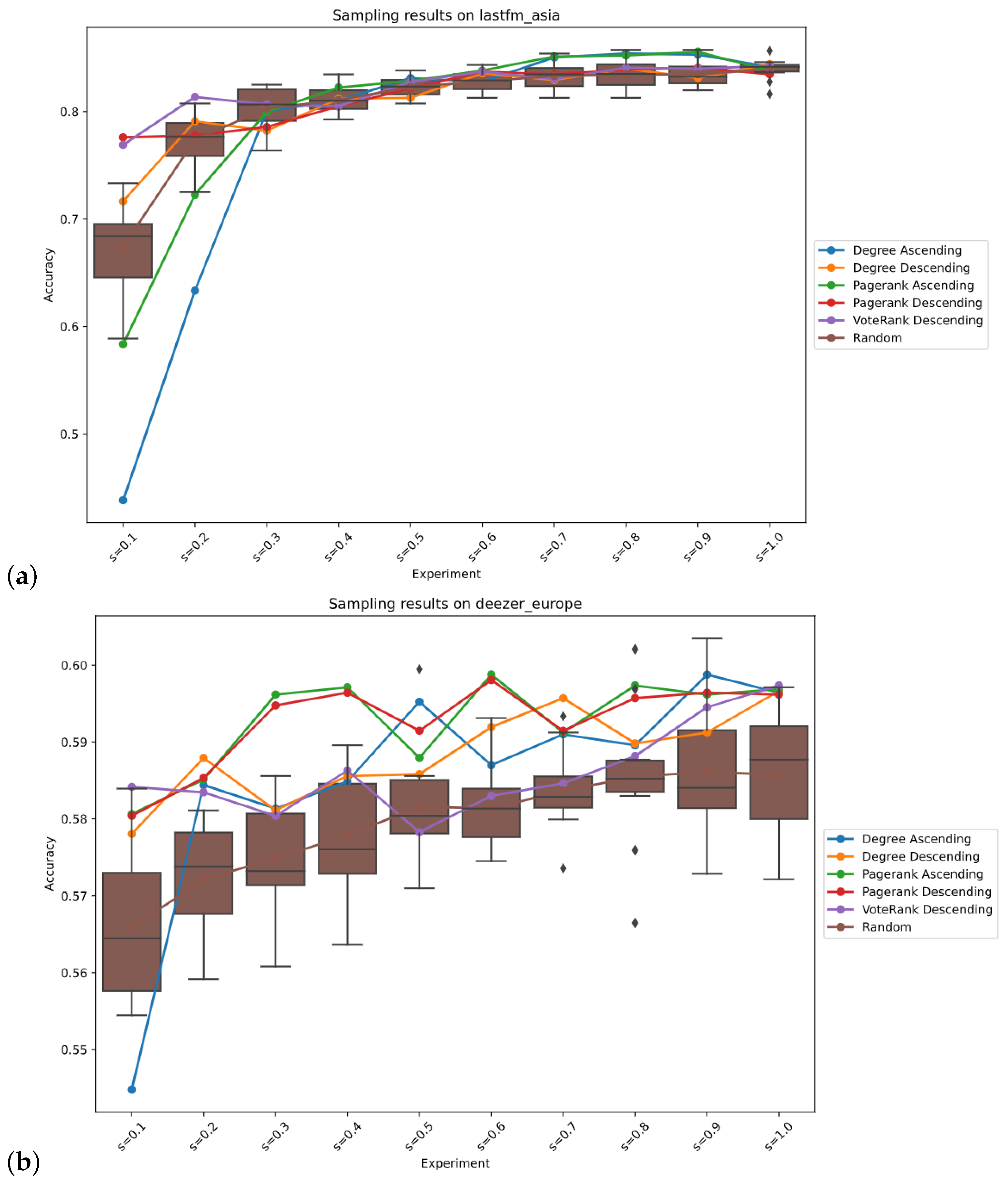
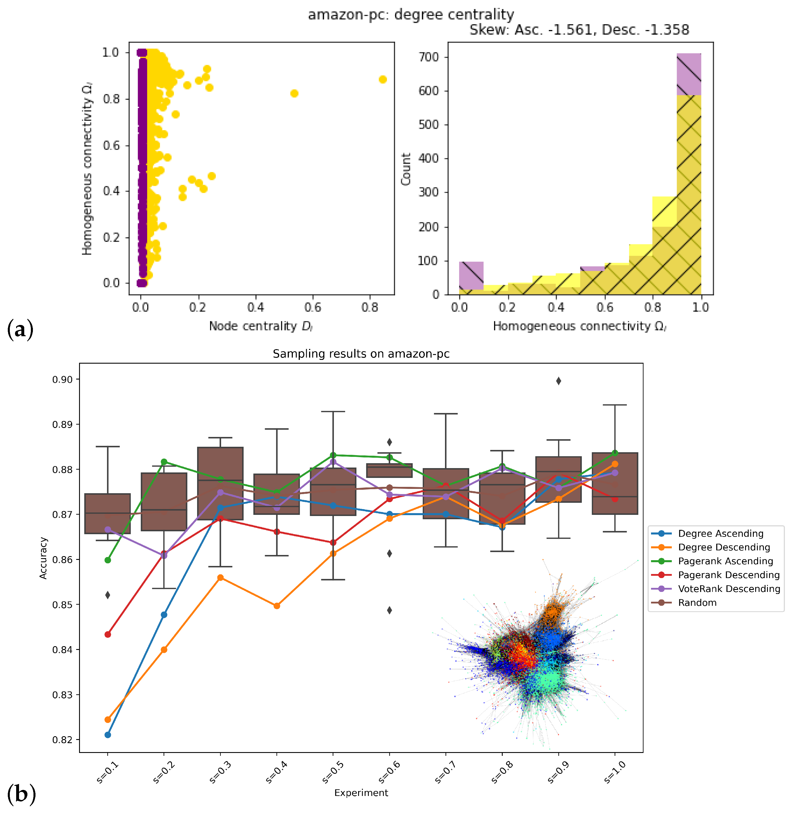
2.2. Sampling Methods
2.2.1. Degree
2.2.2. PageRank
2.2.3. VoteRank
2.3. Simple Graph Convolution (SGC)
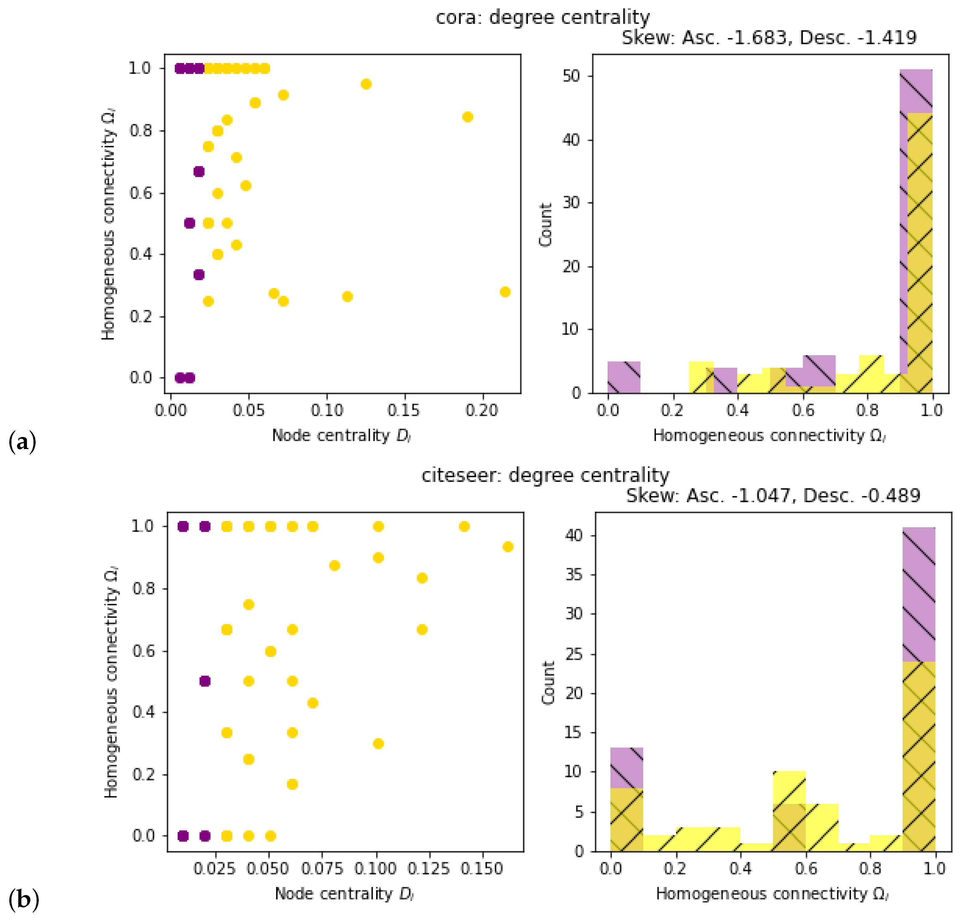
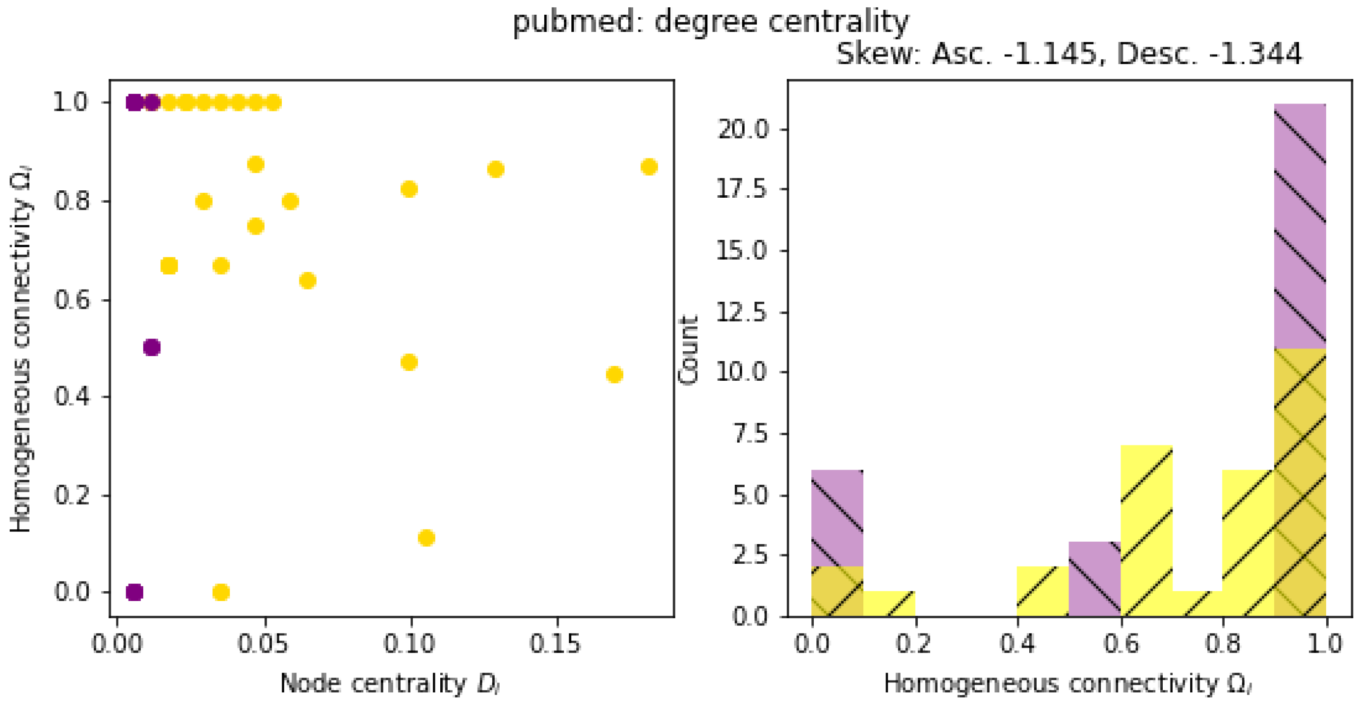
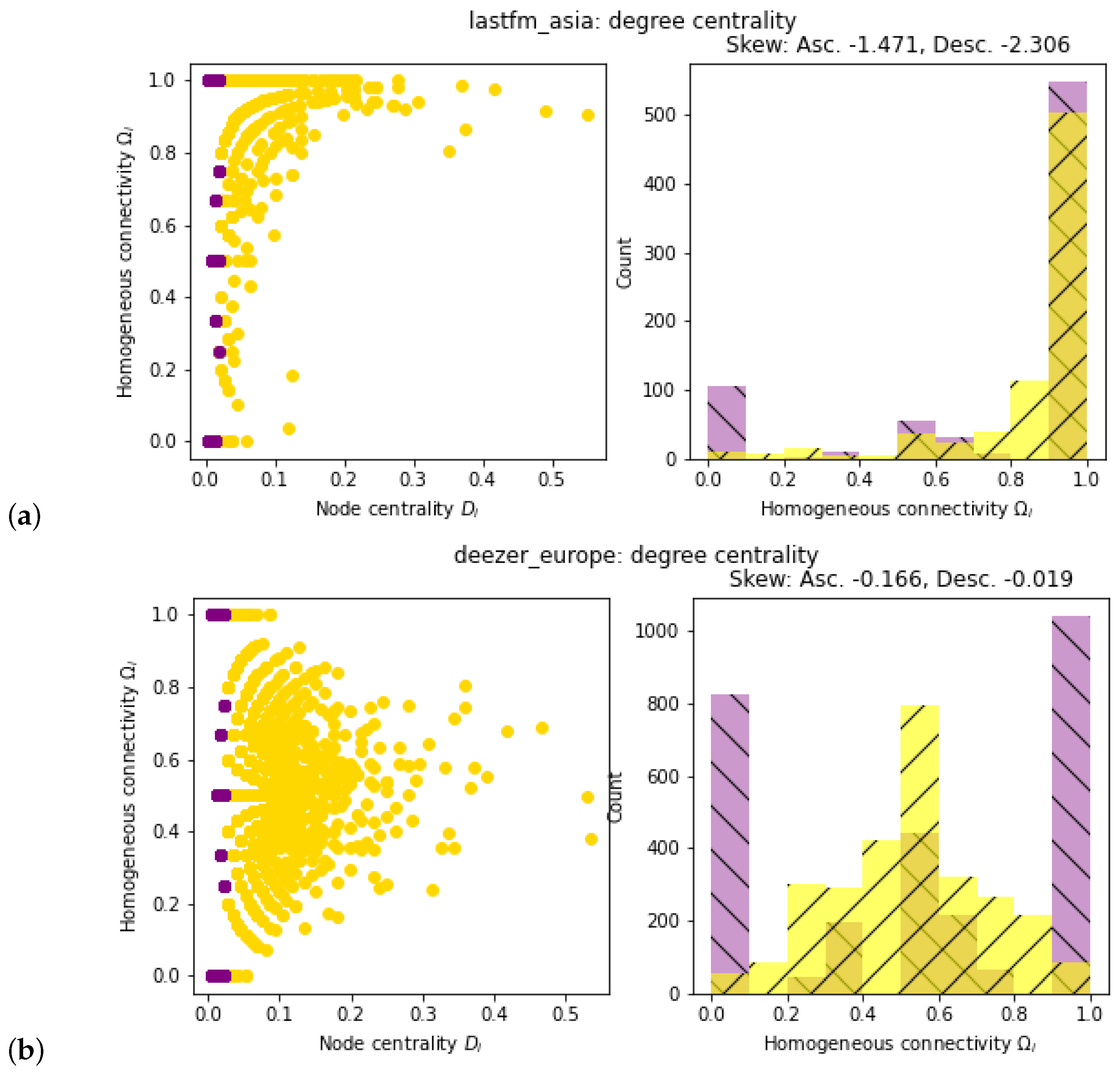
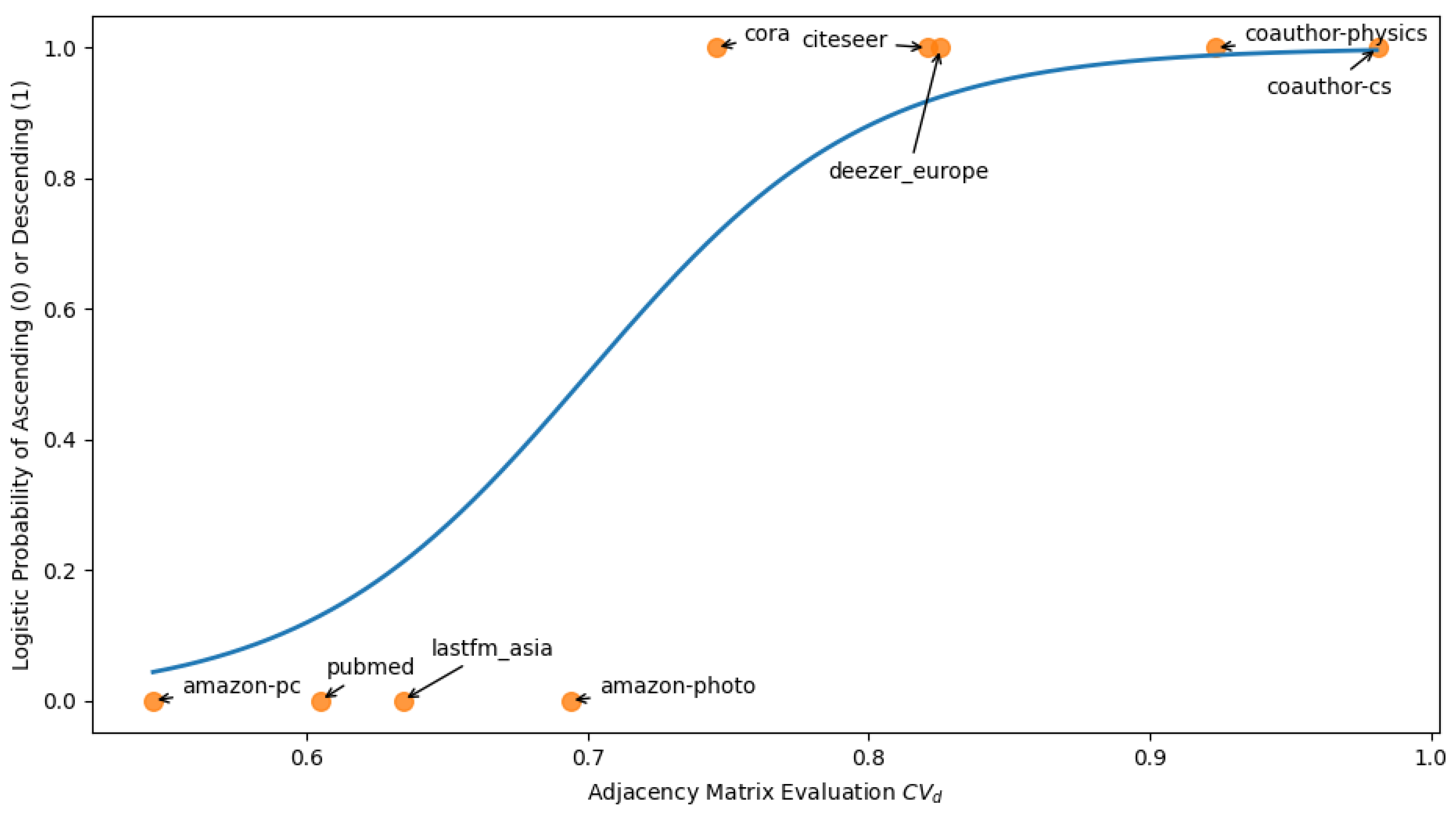
2.4. Evaluation of Network Topology
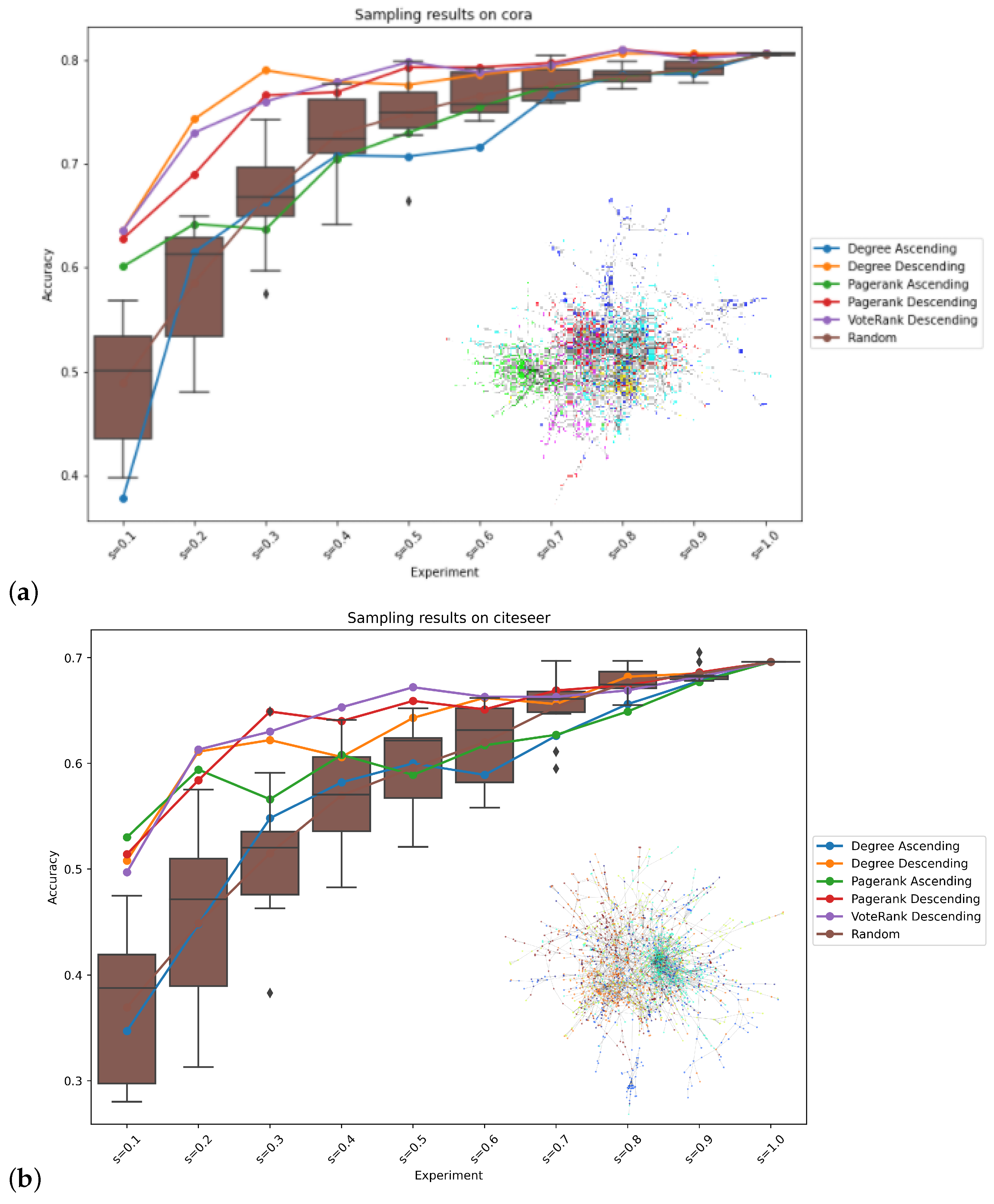
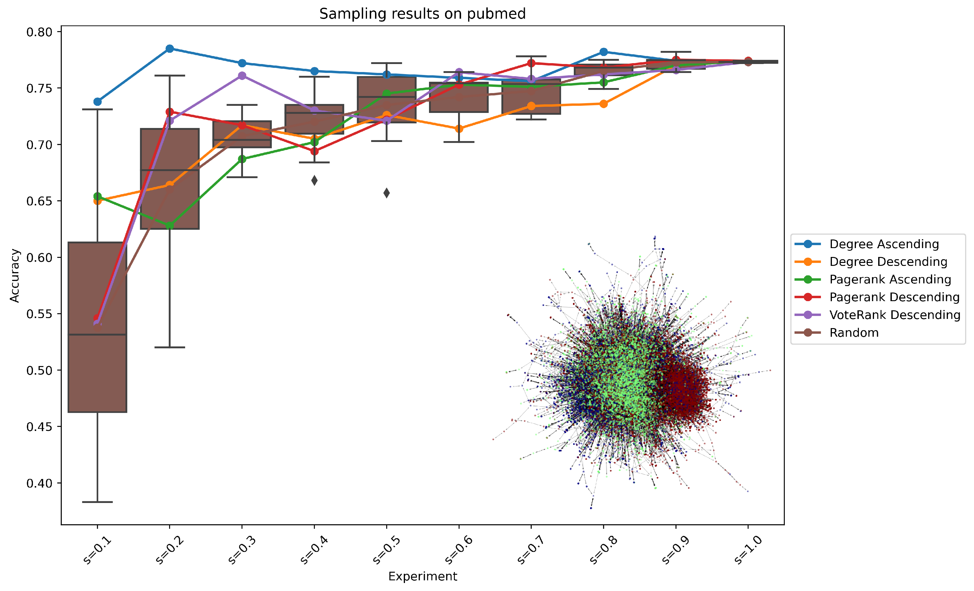
3. Results
4. Discussion
Author Contributions
Funding
Institutional Review Board Statement
Informed Consent Statement
Data Availability Statement
Conflicts of Interest
Appendix A


References
- Newman, M. Networks; Oxford University Press: Oxford, UK, 2018. [Google Scholar]
- Estrada, E. The Structure of Complex Networks: Theory and Applications; Oxford University Press: Oxford, UK, 2012. [Google Scholar]
- Euler, L. Solutio problematis ad geometriam situs pertinentis. In Commentarii Academiae Scientiarum Petropolitanae; 1741; pp. 128–140. Available online: https://scholarlycommons.pacific.edu/cgi/viewcontent.cgi?article=1052&context=euler-works (accessed on 15 April 2021).
- Hoffman, K.L.; Padberg, M.; Rinaldi, G. Traveling salesman problem. Encycl. Oper. Res. Manag. Sci. 2013, 1, 1573–1578. [Google Scholar]
- Schafer, J.B.; Frankowski, D.; Herlocker, J.; Sen, S. Collaborative filtering recommender systems. In The Adaptive Web; Springer: Berlin/Heidelberg, Germany, 2007; pp. 291–324. [Google Scholar]
- McPherson, M.; Smith-Lovin, L.; Cook, J.M. Birds of a feather: Homophily in social networks. Annu. Rev. Sociol. 2001, 27, 415–444. [Google Scholar] [CrossRef]
- Kahne, J.; Bowyer, B. The political significance of social media activity and social networks. Political Commun. 2018, 35, 470–493. [Google Scholar] [CrossRef]
- Blondel, V.D.; Guillaume, J.L.; Lambiotte, R.; Lefebvre, E. Fast unfolding of communities in large networks. J. Stat. Mech. Theory Exp. 2008, 2008, P10008. [Google Scholar] [CrossRef]
- Wu, Z.; Pan, S.; Chen, F.; Long, G.; Zhang, C.; Philip, S.Y. A comprehensive survey on graph neural networks. IEEE Trans. Neural Netw. Learn. Syst. 2020, 32, 424. [Google Scholar] [CrossRef]
- Wu, F.; Zhang, T.; Souza, A.H.D., Jr.; Fifty, C.; Yu, T.; Weinberger, K.Q. Simplifying graph convolutional networks. arXiv 2019, arXiv:1902.07153. [Google Scholar]
- Zhang, S.; Tong, H.; Xu, J.; Maciejewski, R. Graph convolutional networks: A comprehensive review. Comput. Soc. Netw. 2019, 6, 11. [Google Scholar] [CrossRef]
- Azevedo, A.I.R.L.; Santos, M.F. KDD, SEMMA and CRISP-DM: A parallel overview. In Proceedings of the IADIS European Conference on Data Mining 2008, Amsterdam, The Netherlands, 24–26 July 2008. [Google Scholar]
- Settles, B. Active learning. Synth. Lect. Artif. Intell. Mach. Learn. 2012, 6, 1–114. [Google Scholar] [CrossRef]
- Gal, Y.; Islam, R.; Ghahramani, Z. Deep bayesian active learning with image data. In Proceedings of the International Conference on Machine Learning, PMLR, Sydney, Australia, 6–11 August 2017; pp. 1183–1192. [Google Scholar]
- Siddhant, A.; Lipton, Z.C. Deep bayesian active learning for natural language processing: Results of a large-scale empirical study. arXiv 2018, arXiv:1808.05697. [Google Scholar]
- Settles, B.; Craven, M. An analysis of active learning strategies for sequence labeling tasks. In Proceedings of the 2008 Conference on Empirical Methods in Natural Language Processing, Honolulu, HI, USA, 25–27 October 2008; pp. 1070–1079. [Google Scholar]
- Tang, M.; Luo, X.; Roukos, S. Active learning for statistical natural language parsing. In Proceedings of the 40th Annual Meeting of the Association for Computational Linguistics, Philadelphia, PA, USA, 7–12 July 2002; pp. 120–127. [Google Scholar]
- Madhawa, K.; Murata, T. Active Learning for Node Classification: An Evaluation. Entropy 2020, 22, 1164. [Google Scholar] [CrossRef] [PubMed]
- Wu, Y.; Xu, Y.; Singh, A.; Yang, Y.; Dubrawski, A. Active learning for graph neural networks via node feature propagation. arXiv 2019, arXiv:1910.07567. [Google Scholar]
- Zheng, Q.; Yang, M.; Yang, J.; Zhang, Q.; Zhang, X. Improvement of generalization ability of deep CNN via implicit regularization in two-stage training process. IEEE Access 2018, 6, 15844–15869. [Google Scholar] [CrossRef]
- Kooi, T.; Litjens, G.; Van Ginneken, B.; Gubern-Mérida, A.; Sánchez, C.I.; Mann, R.; den Heeten, A.; Karssemeijer, N. Large scale deep learning for computer aided detection of mammographic lesions. Med. Image Anal. 2017, 35, 303–312. [Google Scholar] [CrossRef] [PubMed]
- Zheng, Q.; Zhao, P.; Li, Y.; Wang, H.; Yang, Y. Spectrum interference-based two-level data augmentation method in deep learning for automatic modulation classification. Neural Comput. Appl. 2020, 1–23. [Google Scholar] [CrossRef]
- Tian, Y.; Luo, P.; Wang, X.; Tang, X. Deep learning strong parts for pedestrian detection. In Proceedings of the IEEE International Conference on Computer Vision, Santiago, Chile, 7–13 December 2015; pp. 1904–1912. [Google Scholar]
- Page, L.; Brin, S.; Motwani, R.; Winograd, T. The PageRank Citation Ranking: Bringing Order to the Web; Technical Report; Stanford InfoLab, 1999; Available online: http://ilpubs.stanford.edu:8090/422/ (accessed on 15 April 2021).
- Zhang, J.X.; Chen, D.B.; Dong, Q.; Zhao, Z.D. Identifying a set of influential spreaders in complex networks. Sci. Rep. 2016, 6, 27823. [Google Scholar] [CrossRef] [PubMed]
- Brown, D.W.; Konrad, A.M. Granovetter was right: The importance of weak ties to a contemporary job search. Group Organ. Manag. 2001, 26, 434–462. [Google Scholar] [CrossRef]
- Shchur, O.; Mumme, M.; Bojchevski, A.; Günnemann, S. Pitfalls of Graph Neural Network Evaluation. In Proceedings of the Relational Representation Learning Workshop, NeurIPS 2018, Montreal, QC, Canada, 3–8 December 2018. [Google Scholar]
- Wang, M.; Zheng, D.; Ye, Z.; Gan, Q.; Li, M.; Song, X.; Zhou, J.; Ma, C.; Yu, L.; Gai, Y.; et al. Deep Graph Library: A Graph-Centric, Highly-Performant Package for Graph Neural Networks. arXiv 2019, arXiv:1909.01315. [Google Scholar]
- Leskovec, J.; Krevl, A. SNAP Datasets: Stanford Large Network Dataset Collection. Available online: http://snap.stanford.edu/data (accessed on 15 April 2021).
- Wu, F.; Zhang, T.; Souza, A.H.D.; Fifty, C.; Yu, T.; Weinberger, K.Q. Simplifying graph convolutional networks. In Proceedings of the 36th International Conference on Machine Learning, ICML 2019, Long Beach, CA, USA, 9–15 June 2019; pp. 11884–11894. [Google Scholar]
- Kipf, T.N.; Welling, M. Semi-supervised classification with graph convolutional networks. arXiv 2016, arXiv:1609.02907. [Google Scholar]
- Pho, P.; Mantzaris, A.V. Regularized Simple Graph Convolution (SGC) for improved interpretability of large datasets. J. Big Data 2020, 7, 1–17. [Google Scholar] [CrossRef]
- McCallum, A.K.; Nigam, K.; Rennie, J.; Seymore, K. Automating the construction of internet portals with machine learning. Inf. Retr. 2000, 3, 127–163. [Google Scholar] [CrossRef]
- Giles, C.L.; Bollacker, K.D.; Lawrence, S. CiteSeer: An automatic citation indexing system. In Proceedings of the Third ACM Conference on Digital Libraries, Pittsburgh, PA, USA, 24–27 June 1998; pp. 89–98. [Google Scholar]
- Sen, P.; Namata, G.; Bilgic, M.; Getoor, L.; Galligher, B.; Eliassi-Rad, T. Collective classification in network data. AI Mag. 2008, 29, 93. [Google Scholar] [CrossRef]
- McAuley, J.; Targett, C.; Shi, Q.; Van Den Hengel, A. Image-based recommendations on styles and substitutes. In Proceedings of the 38th International ACM SIGIR Conference on Research and Development in Information Retrieval, Santiago, Chile, 9–13 August 2015; pp. 43–52. [Google Scholar]
- Kirke, D.M. Gender clustering in friendship networks: Some sociological implications. Methodol. Innov. Online 2009, 4, 23–36. [Google Scholar] [CrossRef]
- Gilmer, J.; Schoenholz, S.S.; Riley, P.F.; Vinyals, O.; Dahl, G.E. Neural message passing for quantum chemistry. In Proceedings of the International Conference on Machine Learning, PMLR 2017, Sydney, Australia, 6–11 August 2017; pp. 1263–1272. [Google Scholar]


| Dataset | Ref. | #Nodes #Edges #Classes | Description |
|---|---|---|---|
| Cora | [33] | 2708 5278 7 | Scientific publications (nodes), defined by a binary vector indicating the presence of words in the paper (features), connected in a paper citation web (edges), and categorized by topic (labels). |
| Citeseer | [34] | 3327 4614 6 | Scientific publications (nodes), defined by a binary vector indicating the presence of words in the paper (features), connected in a paper citation web (edges), and categorized by topic (labels). |
| Pubmed | [35] | 19,717 44,325 3 | Diabetes-focused scientific publications (nodes), defined by a binary vector indicating the presence of words in the paper (features), connected in a paper citation web (edges), and categorized by topic (labels). |
| Amazon-PC | [36] | 13,752 287,209 10 | Computer goods sold at Amazon (nodes), defined by a bag-of-words encoded vector of the product’s reviews, connected with groups of products that are frequently bought together (edges), and grouped into product categories. |
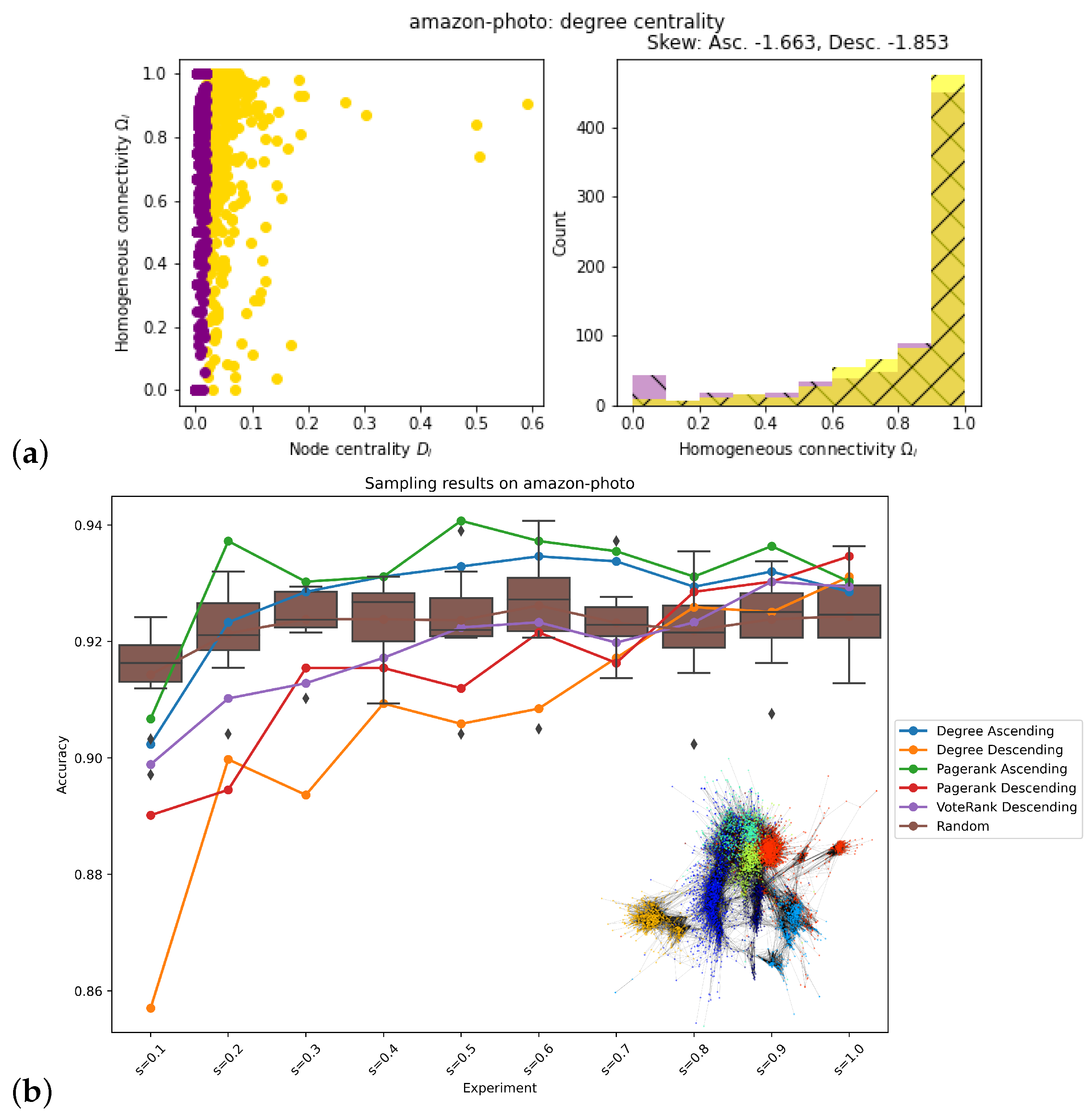
| Amazon-Photo | [36] | 7650 143,663 8 | Photos sold at Amazon (nodes), defined by a bag-of-words encoded vector of the product’s reviews, connected with groups of products that are frequently bought together (edges), and grouped into product categories. |
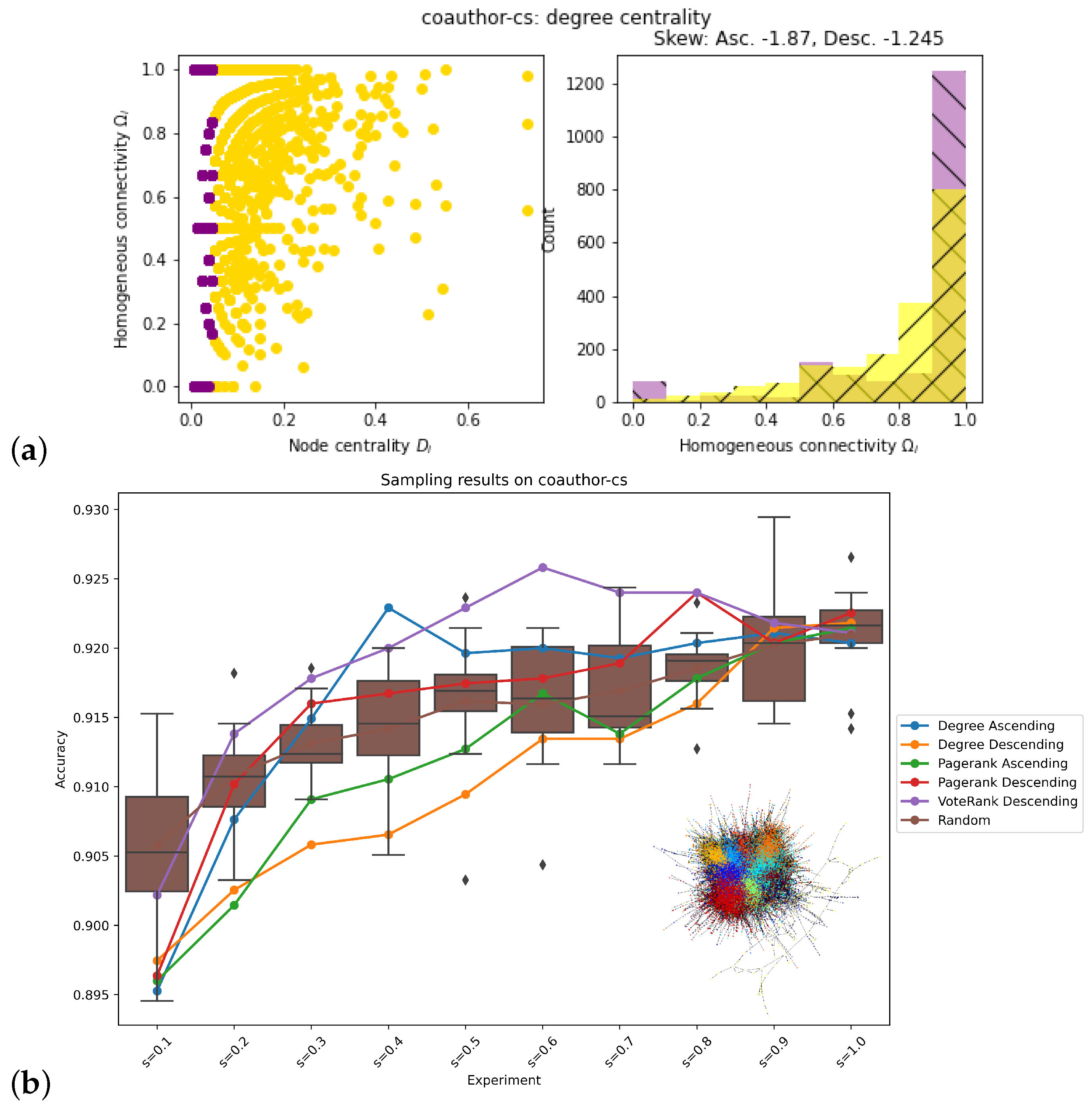
| Coauthor-CS | [27] | 163,788 18,333 15 | Authors (nodes) of computer science papers, defined by a vector of keywords in their published papers, connected by coauthorship (edges), and categorized by the author’s most active field of study. |
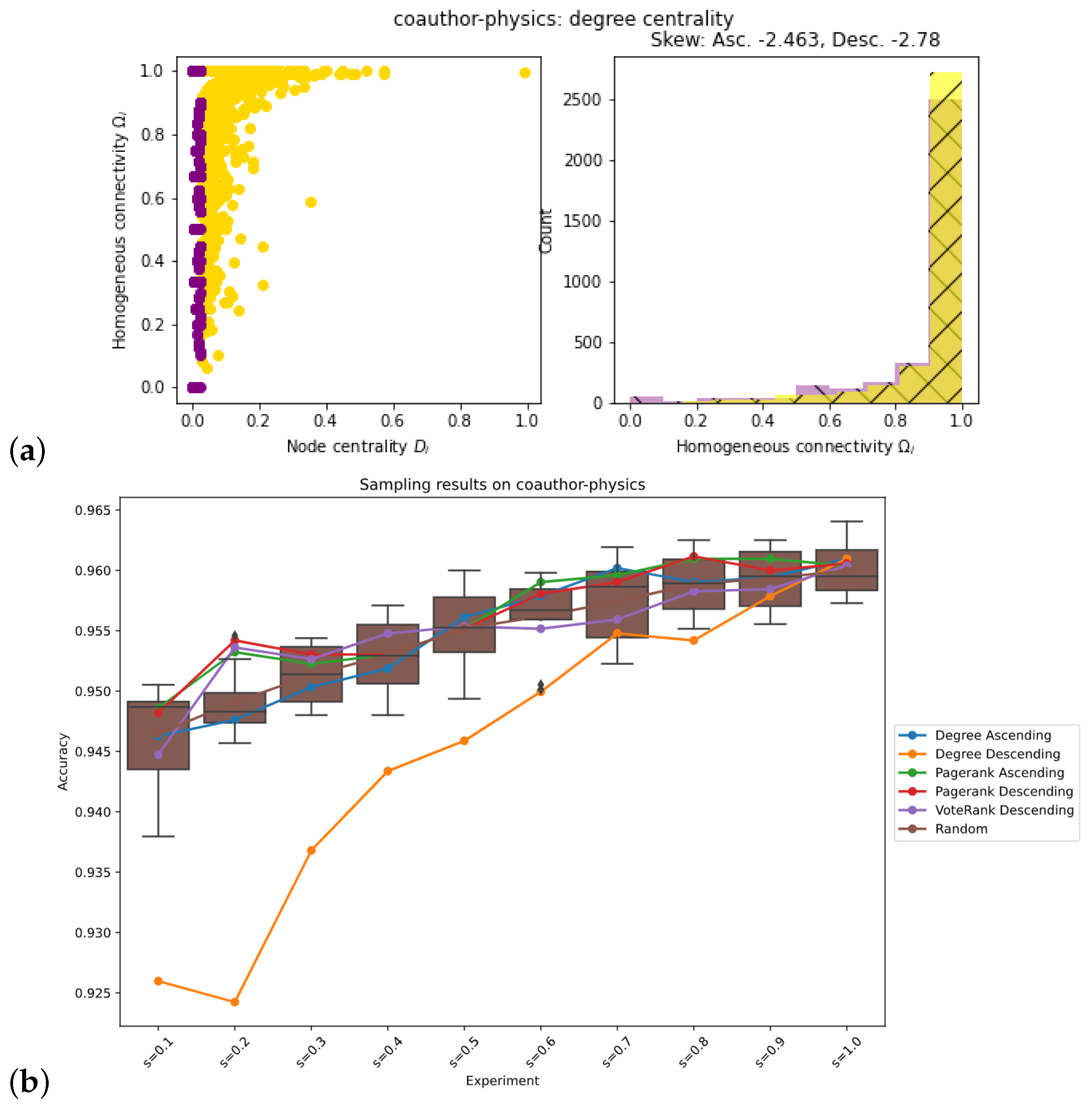
| Coauthor-Physics | [27] | 34,493 495,924 5 | Authors (nodes) of physics papers, defined by a vector of keywords in their published papers, connected by coauthorship (edges), and categorized by the author’s most active field of study. |
| Lastfm-Asia | [33] | 7624 27,806 18 | Social network users (nodes) using LastFM, defined by their artists-of-interest, connected by their mutual followers (edges), and categorized by the user’s location. |
| Deezer-Europe | [33] | 28,281 92,752 2 | Social media users (nodes) using Deezer, defined by their artists-of-interest, connected by mutual followers (edges), and categorized by gender. |
| Dataset | Prediction | Actual |
|---|---|---|
| Cora | Descending | Descending |
| Citeseer | Descending | Descending |
| Pubmed | Ascending | Ascending |
| Amazon-pc | Descending | Ascending |
| Amazon-photo | Ascending | Ascending |
| Coauthor-cs | Descending | Descending |
| Coauthor-physics | Ascending | Descending |
| Lastfm_Asia | Ascending | Ascending |
| Deezer_Europe | Descending | Descending |
Publisher’s Note: MDPI stays neutral with regard to jurisdictional claims in published maps and institutional affiliations. |
© 2021 by the authors. Licensee MDPI, Basel, Switzerland. This article is an open access article distributed under the terms and conditions of the Creative Commons Attribution (CC BY) license (https://creativecommons.org/licenses/by/4.0/).
Share and Cite
Hopwood, M.; Pho, P.; Mantzaris, A.V. Exploring the Value of Nodes with Multicommunity Membership for Classification with Graph Convolutional Neural Networks. Information 2021, 12, 170. https://doi.org/10.3390/info12040170
Hopwood M, Pho P, Mantzaris AV. Exploring the Value of Nodes with Multicommunity Membership for Classification with Graph Convolutional Neural Networks. Information. 2021; 12(4):170. https://doi.org/10.3390/info12040170
Chicago/Turabian StyleHopwood, Michael, Phuong Pho, and Alexander V. Mantzaris. 2021. "Exploring the Value of Nodes with Multicommunity Membership for Classification with Graph Convolutional Neural Networks" Information 12, no. 4: 170. https://doi.org/10.3390/info12040170
APA StyleHopwood, M., Pho, P., & Mantzaris, A. V. (2021). Exploring the Value of Nodes with Multicommunity Membership for Classification with Graph Convolutional Neural Networks. Information, 12(4), 170. https://doi.org/10.3390/info12040170