Towards a Predictive Bio-Inspired Navigation Model

Abstract

This paper presents a novel bio-inspired predictive model of visual navigation inspired by mammalian navigation. This model takes inspiration from specific types of neurons observed in the brain, namely place cells, grid cells and head direction cells. In the proposed model, place cells are structures that store and connect local representations of the explored environment, grid and head direction cells make predictions based on these representations to define the position of the agent in a place cell’s reference frame. This specific use of navigation cells has three advantages: First, the environment representations are stored by place cells and require only a few spatialized descriptors or elements, making this model suitable for the integration of large-scale environments (indoor and outdoor). Second, the grid cell modules act as an efficient visual and absolute odometry system. Finally, the model provides sequential spatial tracking that can integrate and track an agent in redundant environments or environments with very few or no distinctive cues, while being very robust to environmental changes. This paper focuses on the architecture formalization and the main elements and properties of this model. The model has been successfully validated on basic functions: mapping, guidance, homing, and finding shortcuts. The precision of the estimated position of the agent and the robustness to environmental changes during navigation were shown to be satisfactory. The proposed predictive model is intended to be used on autonomous platforms, but also to assist visually impaired people in their mobility.

1. Introduction

Navigating in an environment, whether indoor or outdoor, is a fundamental task for autonomous robotic systems and a vital task for many species. Autonomous robotic systems most commonly use SLAM (Simultaneous Localization And Mapping) approaches [1,2] in order to constantly estimate their position in an unknown environment. Various active and passive sensors are employed in order to build a precise global map of the investigated environment. Visual features/cues (interest points and/or landmarks) are frequently used to model and recognize places, while odometry data is used to track the local motion of the robot. A navigation model is continually updated based on location recognition and odometry data, the robot being simultaneously localized within the map. Each node of this graph represents a particular waypoint, while edges represent accessibility between waypoints. Once the navigation graph is constructed, it is possible to specify goal vertices, and navigate to them autonomously. However, measurement errors accumulate over time and lead to a drift in the estimated position, causing discrepancies in the map of the environment. Therefore, alleviating these discrepancies is a major question in the field of SLAM systems. High precision and minimal computational costs are the main requirements for such navigation. Finally, these approaches usually perform better in environments of limited size [3].

Another class of approaches for the autonomous navigation problem takes inspiration from the very decentralized navigation systems of mammals which allow navigation in large-scale environments. Instead of creating a global map during the exploration of the environment, these approaches generate a graph model, where nodes are local representations (i.e., at a limited distance) of the observed environment in that node.

This class of approaches is inspired by place cells [4], a spatially correlated neuron found in mammalian brains. Navigation based on this model consists of following a path (a sequence of connected nodes) in a given mobility graph, from one node to the next, from the current position to the destination node. However, several problems arise when navigating in a large (theoretically unlimited) space due to the limited resources of a mammalian brain:

• How can the graph model an infinite space with limited capacity?
• When should a new node be added to the graph? Conditions must be identified in order to define a distance (fixed or not) between nodes;
• How to control the navigation in a physical environment using the navigation graph? In other words, how to match the physical location to a graph node to obtain the direction and distance values necessary to reach the next node in the path?
• Knowing that the visual system of the majority of mammals do not have a field of view covering the ${360}^{\circ }$, how to integrate newly discovered visual cues when moving through a previously visited node, with a different orientation?

This paper proposes new answers to the above questions through its novel predictive approach to indoor and outdoor navigation based on collaboration between place cells, grid cells and head direction cells [5]. The proposed model is in-line with bio-inspired approaches, and aims to model and design robust systems which can be used on robotic platforms and on assistive devices for people with visual impairment, spatial neglect, or aphantasia [6,7,8]. Our goal of providing assistance to visually impaired people adds extra constraints to our model such as: the visual system must have a narrow field of view (as omnidirectional cameras are impractical to carry on a person), movements are more varied than on a wheeled robotic platform, and there is no absolute odometry (e.g., wheel encoders).

This paper is organized as follows: Section 2 outlines a state of the art on some bio-inspired navigation models. Section 3 gives an overview of our predictive model and its main properties. Section 4 details the computational principles of the proposed predictive model, while Section 5 describes a preliminary implementation of the proposed model and provides the results of its experimental evaluation in a simulated 2D environment. Finally, Section 6 summarizes the obtained results and discusses some use cases of the proposed model and its potential future developments.

2. State of the Art on Bio-Inspired Navigation Models

Several vision-based navigation models try to mimic the functioning of the brain’s navigation system, both to develop efficient navigation models and to validate biological hypotheses. After the discovery of place cells [4] and grid cells [9], many models inspired by mammalian navigation abilities were proposed. All of them target both the better understanding of cognitive navigation processes which underpin the real navigation and the development of more robust and efficient navigation models.

These approaches integrate more or less accurately the properties of various specialized neurons involved in the memorization of locations and in the construction of a topological representation of the environment that is robust to motion drift and environmental changes. However, these models do not completely answer all the questions listed above.

Gaussier et al. [10], Jauffret et al. [11], Zhou et al. [12,13], and Chen and Mo [14] proposed neurobiological models of place cells and grid cells allowing the encoding of a robot’s environment and navigating in it. Several implementations demonstrated that these systems can construct and maintain stable models for long periods [15]. They however require an omnidirectional or pan camera to acquire the full context at once. These cameras are not practical for use in a portable or wearable device.

RatSLAM [16] and its subsequent improvements (e.g., SeqSLAM [17], Tang et al. [18]) are approaches that rely on a 3D attractor network of pose cells, inspired by grid cells properties, and experience maps to encode position and orientation. Cells of this network record observed images, allowing them to recognize visited places while providing position and orientation information. These systems are able to map very large environments and track positions even through environmental changes. They provide an answer to question 2 with the use of cell networks providing a constant distance between places. However, these models are constrained to forward-moving vehicles (e.g., cars) and thus cannot be used for pedestrian motion.

The predictive model of mobility presented here proposes a new answer to question 2, and solutions for the other three questions.

3. Predictive Bio-Inspired Model of Mobility: Overview

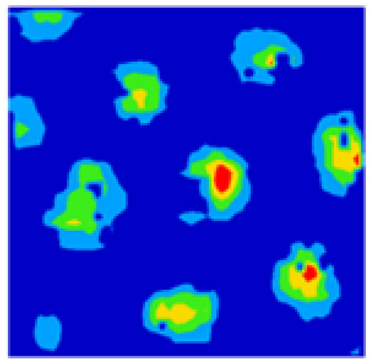
The predictive model proposed in this paper is in-line with the bio-inspired approaches, and is rooted in a sensorimotor theory of perception [19]. The principles underlying this model incorporate properties observed in a developmental architecture proposed by Georgeon and Aha [20], and a structure, called Space Memory [21], which specifies how the relation between an agent’s actions and the environment’s spatial geometry can be learned without any prior knowledge.

The proposed navigation model provides answers to the questions identified in Section 1. Several elements intervene in our model: grid cells (Section 3.1), grid cell firing model during the navigation (Section 3.2), localization in space and movement prediction (Section 3.3).

3.1. Grid Cells

The proposed model takes inspiration not only from the place cells but also from another type of cell linked to mammalian navigation: grid cells. The grid cells are involved in estimation and integration of movements in space. The activation field of grid cells is organized as a hexagonal grid (Figure 1). Grid cells close to each other in the brain possess the same spatial properties (spacing between peaks in the activation field, orientation of the grid) except they are not in phase i.e., their grid is shifted spatially from each other. Groups of these cells are called modules and together they cover all physical space. When an agent moves, it goes in and out of the activation field of a module’s cells. The movement of the agent can be estimated from the successive activations of the grid cells in the same module.

Each grid cell module “represents” a small area around a given position, and has its specific spatial characteristics (the distance between 2 adjacent activation peaks of its grid cells called the spacing, and the absolute orientation to the physical space). The sequence of activation of Grid Cell of the module can be used to estimate the displacement in the covered area.

The grid cell module wraps space in a toric manner, thus repeats infinitely. Therefore, the infinite physical space of navigation can be continually projected on the same physiological support of the mental navigation space. This representation answers question 1 of Section 1.

Several modules of grid cells co-exist in the brain and provide different spatial information of the same physical position (at different scales). As the repetition of modules are different, due to their different spacings, the combination of position provided by each module helps to characterize the position in the environment despite the repetition of these modules.

3.2. Grid Cells Firing during the Navigation

During navigation, the activations of successive grid cells allow the estimation of the movements of the agent in space. Since the module constitutes a toric space, the same grid cell will activate in a periodic manner when the animal travels larger distances than the module can represent. This toric property means that an arbitrary cell can be designated as the center of the module, and the furthest cells from this center cell are the border grid cells. The center of a module can be redefined at any moment. By associating a given position of space to the center place cell of the module, it is possible to define the movement and the position of the agent relative to this position, in the area bounded by border place cells.

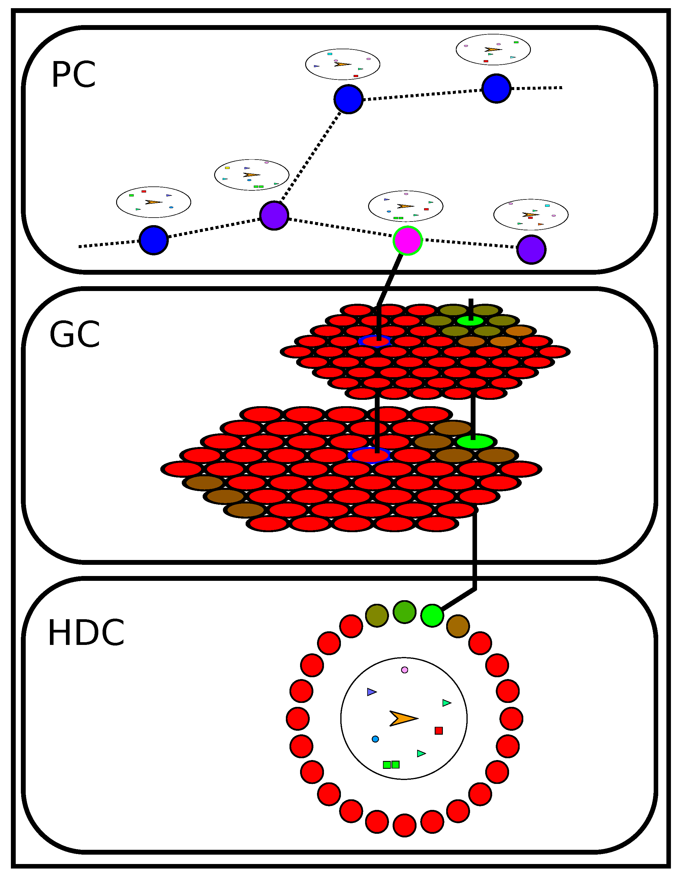
3.3. Localization and Movement Prediction: A Cooperation between Place Cells, Grid Cells and Head Direction Cells

A place cell is defined as a structure associated with a specific position of space that records the environmental context observed when the agent was on this position. This recorded context is compared with the currently observed context to define the firing rate of the place cell: when the observed context is closed from the recorded context, the firing rate increases, allowing recognition of the position when the agent approaches it.

A set of place cells can be considered to be a graph representation of the environment (Figure 2). Two place cells (two nodes of the graph) are connected if is possible to move from a place cell’s position to the other place cell’s position. Even though more than one place cell can fire at time t (which is expected in redundant environment), the model considers only one place cell as active at t. The active place cell indicates the current local reference for position estimation. The active place cell only changes when the agent approaches the next place cell on the graph.

When starting a new navigation graph, the system adds a new place cell, and one grid cell from each module, designated as the center, is associated with this place cell (Figure 3). Each grid cell of a module gets the recorded context of the place cell and uses the offset (phase difference) with the center grid cell to predict the expected environmental context that could be observed at the position characterized by this grid cell. Each grid cell then compares its predicted context with the currently observed context to define its activity (firing rate). It is then possible to estimate (via interpolation) the agent’s position near the place cell by measuring the activity of grid cells.

This position measurement is however constrained to a finite distance from the place cell. Once a border grid cell is reached, the module limit is reached. A new place cell is then added to the navigation graph. This place cell stores the current observed context and links to the currently most active grid cell of each module, which becomes the new center of its module.

The above approach solves question 2: when should a new node be added to the graph. It should be observed that the distance between place cells is given by the size of the local space represented by the smallest used module. The relative position between two place cells is given by the offset that separates their respective associated grid cells, and the agent’s position between two place cells is estimated by the grid cells.

The model presented so far does not take into account the orientation of the agent’s movement. To identify the orientation, artificial head direction cells are added. In our model, each head direction cell is characterized by a predefined angle of rotation; all the head direction cells cover the 360 degrees uniformly. Each head direction cell generates a rotated context from the currently observed context (Figure 3). The rotated contexts are then compared to the predicted contexts (from the grid cells), the orientation-grid pair with the highest activity gives the orientation and position relative to the current active place cell.

Figure 3 schematizes the cooperation of the “brain substrate” of the proposed model to control the navigation and suggests an answer to question 3 related to the control of navigation. The active place cell sends its context to the grid modules. The predicted contexts produced by grid cells from active place cell’s recorded context and the predicted context produced by head direction cells from observed context are then compared to predict the location and orientation of the agent around the active place cell’s position.

As the position around the place cell can be estimated, it is possible to predict the position of currently observed visual cues if they were observed from the place cell’s initial position, and thus, to add newly observed cues to the recorded context of this place cell. This answers our question 4: how to integrate new visual cues.

This predictive model of navigation has many advantages: predicted contexts are computed only once, when the active place cell changes, and even if the environment changes (e.g., added or removed points of interests), the system will still be able to easily find the current position by observing only the points of interest close to the expected ones. Moreover, no matter the differences with the previously stored context, there will always be a context more active than the others.

4. Predictive Model of Navigation: A Computational Approach

This section presents a computational definition of the proposed predictive model of navigation. This model involves interactions between the three types of navigation cells. Section 4.1 defines the environmental context of a place cell; Section 4.2 models the orientation tracking using head direction cells; Section 4.3 explains how the place cells recognize a context; Section 4.4 outlines how the grid cells work to precisely localize the agent around the considered place cell; the subsequent sections show how a new place cell is added during the navigation (Section 4.5), how place cells are linked in a mobility graph (Section 4.6) and how the agent’s position is tracked using the mobility graph (Section 4.7); finally, Section 4.8 shows how the mobility graph supports three basic navigation tasks: reaching a goal, homing and shortcut detection.

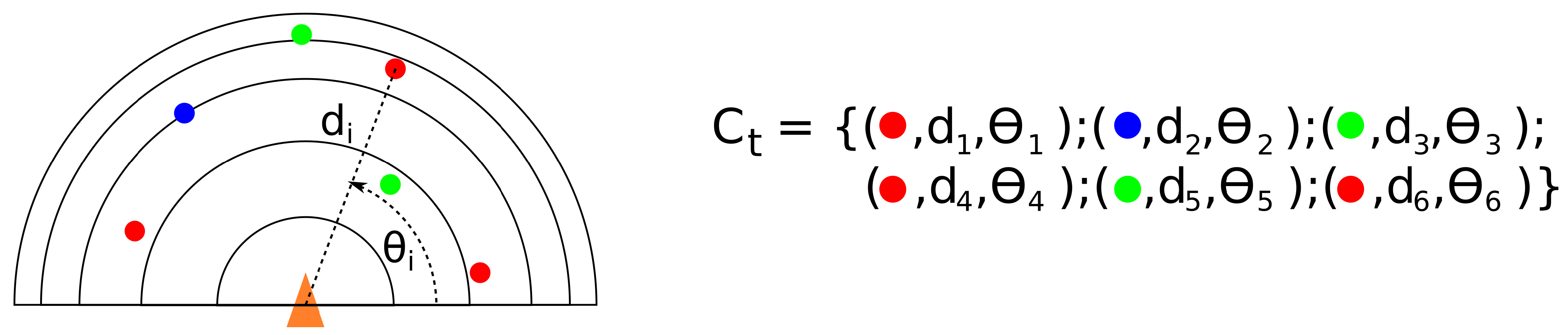
4.1. Environmental Context

We define an environmental context as a representation of the surrounding environment of the agent in its egocentric reference. A context is a set of salient features that can be identified and localized in the space surrounding the agent. Formally, the environmental context is a set of pairs $(e,p)$ where e is the type of element (its color for instance) and p its position in the agent’s egocentric reference frame.

During navigation, the visual system continually produces a context $C_t$ containing the currently observed visual cues (the aforementioned e). This context is defined in egocentric reference frame. Figure 4 presents the context $C_t$ perceived by the agent (orange triangle) at time t; it contains three red elements ($e_1$, $e_4$, $e_6$), one blue element $e_2$ and two green elements ($e_3$ and $e_5$).

The different structures of the navigation model produces predictions by applying spatial transformations to the elements of the context. This model incorporates properties observed in the model of space memory proposed by Gay et al. [21], and more specifically, properties observed in a subsequent work [23] that showed that complex spatial transformations, such as reference changes, can be learned by experience and exploited to predict environmental contexts in other positions. From this model, we extract two relevant properties:

• a movement m in space is strictly equivalent to the position p that it is allowed to reach;
• any position p in the surrounding space can be updated to $p^{\prime }$ through a movement m; this is expressed with $p+m\to p^{\prime }$.

4.2. Tracking Orientation: Head Direction Cells

The head direction cells are defined in our model as structures encoding a specific rotation in allocentric reference frame; the set of head direction cells give a regular discretization of the $[0;2\pi ]$ interval (Figure 5). These head direction cells are used to generate rotated contexts. For a given context C, each head direction cell H associated with rotation moment ${\varphi }_H$ will define a rotated context $C_H=\left\{(e,p^{\prime })\right|p+{\varphi }_H\to p^{\prime }\}$.

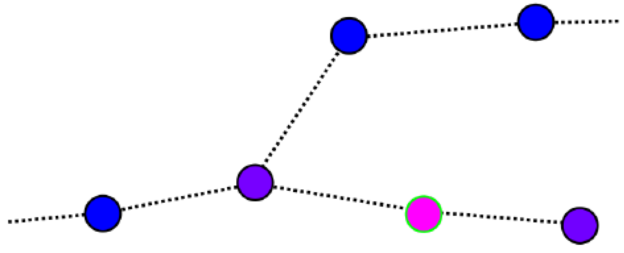
4.3. Recording and Recognizing Contexts: Place Cells

Our model considers place cells as structures encoding environmental contexts. The purpose of a place cell P is to recognize its associated place in space by comparing its recorded context $C_P$ with the current perceived context $C_t$. Formally, a place cell is a function $P:\left\{C\right\}\to [-1;1]$ that computes the similarity ($P\left(C\right)>0$) or dissimilarity ($P\left(C\right)<0$) between $C_t$ and $C_P$ (Section 5 gives an example of implementation for P). To make the place cell activity $P_a$ invariant to rotation, $P_a$ is computed using the rotated context $C_H$ that gives the highest value:

$$P_a\left(C_t\right)=ma{x}_{H}P\left(C_H\right)$$

(1)

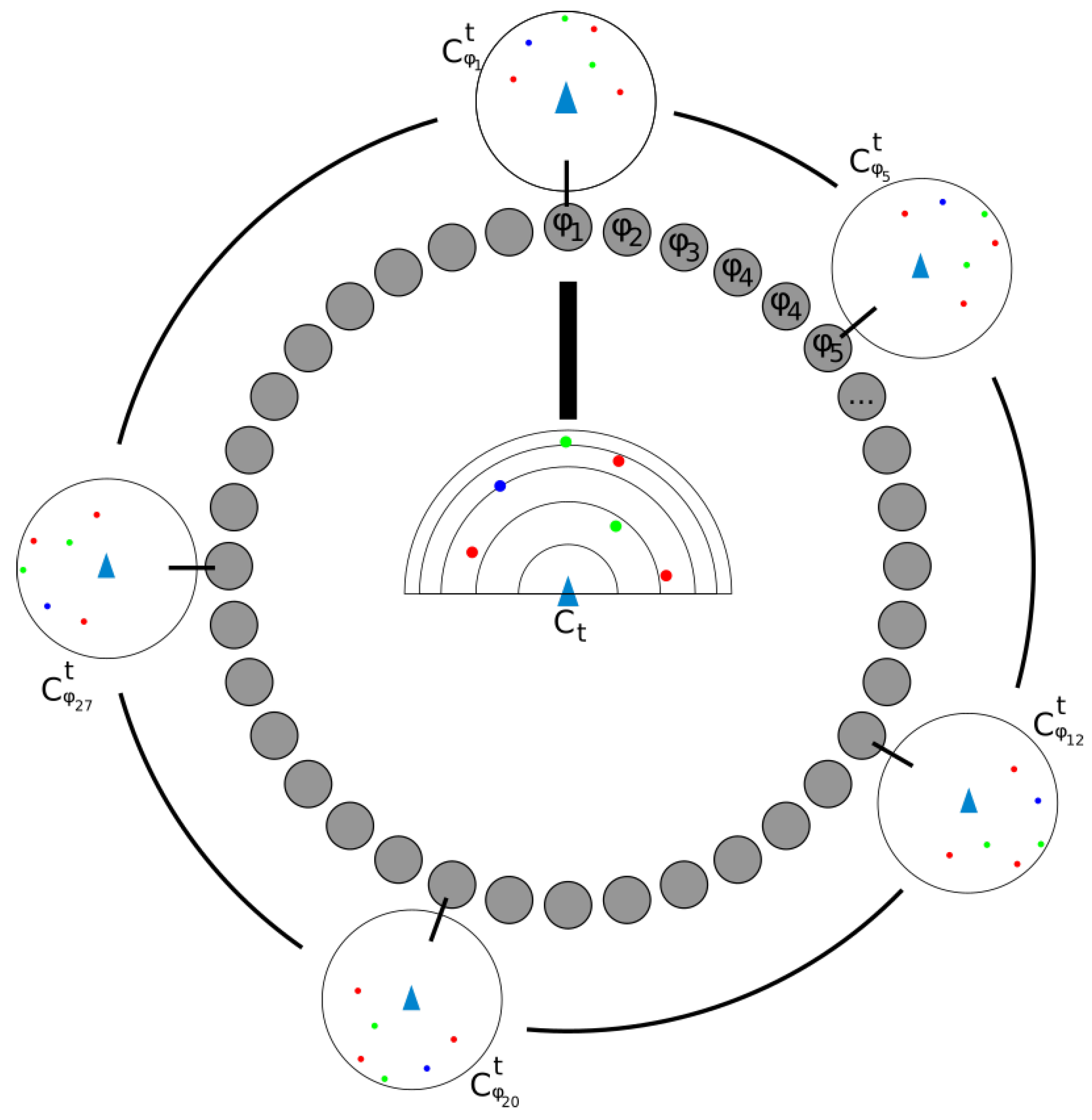
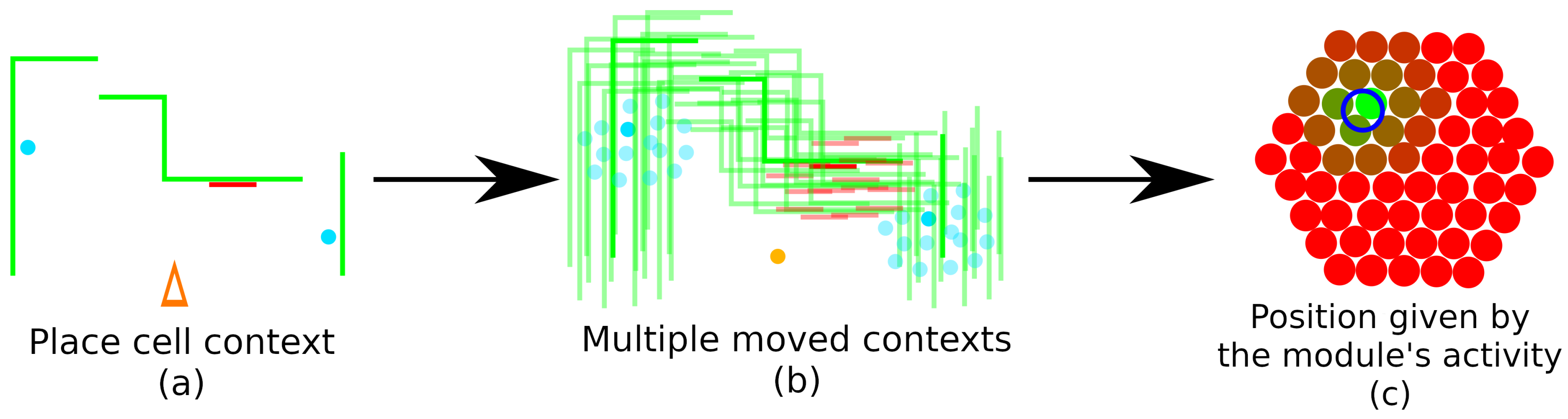
4.4. Localizing Around a Place Cell: Grid Cells

A place cell can indicate when the agent is in its receptive field (the set of points of space in which this place cell is active), but does not inform on the agent’s location relative to the place cell. This information, however, is needed to add newly discovered elements to the place cell context (e.g., when the agent performs a rotation). To overcome this limitation, we drew inspiration from the brain’s grid cells.

In our model, grid cells intend to localize position and integrate movements of the agent around a place cell. As said above, grid cells are grouped into discrete modules [24]. Like a place cell, a grid cell G computes the similarity between a context $C_G$ received from the currently active place cell, and the current context $C_t$. However, grid cells differ from place cells in three ways: they do not have associated contexts, they do not need to compute dissimilarities (only similarity), and their receptive field cover a smaller area of space. Formally, a grid cell is a function $G:{\left\{C\right\}}^2\to [0;1]$.

The grid cell localization procedure is based on the following assumption: each pair of grid cells $(G_i,G_j)$ of the same module corresponds to a unique, known, movement in space, noted $m_{i,j}$, considered to be the shortest movement separating their receptive fields (on the toric surface). Each place cell is associated with one grid cell of one or multiple modules. When the agent is close to a place cell $P_k$ storing the context $C_{P_k}=\left\{(e,p)\right\}$ and associated with a grid cell $G_i$, it is possible to define, for each grid cell $G_j$ of the same module as $G_i$, a modified context $C_{G_j}=\left\{(e,p^{\prime })\right|p+m_{i,j}\to p^{\prime }\}$. Such modified contexts are predictions on the context that should be observed when moving around the place cell.

Therefore, the activity of every grid cell $G_j$ of the module(s) is computed using the rotated contexts $C_{H_k}$ from head direction cells. The pair of head direction cell and grid cell $(H_{k_{max}},G_{j_{max}})$ providing the greatest activity (2) in the current context $C_t$, gives the orientation ${\varphi }_{max}$ and position $m_{max}$ of the agent in the current place cell’s reference frame.

$$(H_{k_{max}},G_{j_{max}})/G_{j_{max}}(C_{H_{k_{max}}},C_{G_{j_{max}}})=\underset{H_k,C_j}{max}{G}_j(C_{H_k},C_{G_j})$$

(2)

The exact position and orientation of the agent can then be interpolated using head direction cells and grid cells that are close to $H_{k_{max}}$ and $G_{j_{max}}$. Figure 6 illustrates how grid cell prediction works. By knowing the position and orientation in the place cell’s reference, it is possible to add newly observed elements $(e,p)$ of context $C_t$ as elements $(e,p^{\prime })$ where $p-(m_{max}+{\varphi }_{max})\to p^{\prime }$. This makes possible to update the context of the current place cell.

4.5. Adding New Place Cells to the Navigation Graph

Grid cells are also used to determine when a new place cell has to be added: as the current place cell defines the center of a grid cell module (i.e., its associated grid cell), it also defines border grid cells. These cells are the grid cells with the greatest distances to the module center (Figure 7). Reaching one of these border grid cells indicates that the agent is moving out of the module’s area of coverage centered on the current place cell (we only consider the module with the smallest spacing among those associated with the current place cell). Such situation will prompt a new place cell to be created and associated with the current most active grid cell. This initially border grid cell becomes the new center of the module, as shown in Figure 7. The previous place cell is then connected to the new one, with the spatial transformation separating them encoded by their associated grid cell. Therefore, while exploring the environment, the system progressively constructs a sequence of place cells encoding the performed path based on grid cell modules. A consequence of this mechanism is that the distance between place cells is nearly constant and independent from the estimated distance to observed elements, and relies solely on used grid cell modules.

4.6. Connecting Place Cells

Place cells are used to recognize known places. When reaching a border grid cell, the system will first check for place cells with strong activities. When the most active place cell has an activity higher than a predefined threshold, indicating that a sufficient number of cues of its context can be recognized in the environment, the current place cell is linked to the recognized place cell. Several methods to improve place cell recognition are discussed in Section 6.

4.7. Position Tracking in the Place Cell Graph

When freely moving in a known part of the environment, the localization system keeps track of the position by updating the current place cell. When the agent is closer from a neighbor place cell than the current one (based on the grid cell activities), this neighbor cell becomes the new current place cell. The place cell subsequently loads its context in the grid cell module which then helps re-calibrating the estimated position. This principle thus uses the relative position of place cells instead of their activity, and allows tracking the position even with very few visual cues and environmental changes. Indeed, the system only considers elements that are close to the predicted position; missing, new and displaced elements are ignored and possibly removed from current place cell’s context (as observed in experiment in Section 5.5). The system can also correct errors in the place cell graph, disconnecting neighbor place cells that have a negative activity when approached.

4.8. Using the Navigation Graph

A navigation mechanism allows the agent to autonomously move through a sequence $S=[P1,\cdots ,Pn]$ of place cells. In the context of a place cell $P_k\in S$, associated with the grid cell $G_k$, the mechanism considers

• the next place cell $P_{k+1}$ and its associated grid cell $G_{k+1}$ to define the relative position $m_{k,k+1}$ between $P_k$ and $P_{k+1}$;
• the current most active grid cell $G_c$ to define the relative position $m_{k,c}$ of the agent.

The position $m_{c,k+1}$, sum of $m_{c,k}$ and $m_{k,k+1}$, provides the orientation and distance to reach the next place cell. When the agent is close to the place cell $P_{k+1}$, this place cell becomes the reference. The process is repeated to move from $P_{k+1}$ towards $P_{k+2}$. Please note that unlike free navigation, the system will only consider the next place cell of the sequence, inhibiting other neighbors even though they could be closer.

$$\varphi +m_{c,0}+\sum _{P_k\in S_{0,i}}{m}_{k,k+1}\to p_{P_i}$$

(3)

where

• $\varphi$ is the estimated orientation,
• $m_{c,0}$ the estimated position in the current place cell $P_0$,
• $S_{0,i}$ the shortest sequence of place cells between $P_0$ and $P_i$.

These positions can then be compared with the current context $C_t$: when a position $p_{P_i}$ can be directly reached (i.e., no observable elements between the agent and $p_{P_i}$), then $P_i$ can be accessed in straight line. The agent then performs this movement, and continuously updates its position using the odometry provided by existing or newly added place cell, until it can visually recognize a place cell of the navigation graph.

4.9. Homing without Visual Context: Visual Odometry

When the visual field is too narrow to record and recognize contexts in a reversed direction, moving back cannot rely on visual cues. The homing mechanism makes it possible to move a sequence of place cells backwards to return to the starting position without knowing the environmental context, based on visual odometry.

This mechanism uses grid cells that are associated with place cells to define the movement to produce. Starting from the last place cell of the sequence, the previous place cell designates the grid cell that must be reached, giving the direction and distance to reach the estimated position of the previous module center. When the agent reaches this grid cell, the previous cell in the sequence indicates a new grid cell to reach, and so on until reaching the estimated position of the first place cell of the sequence. During this homing move, if the agent’s visual field is narrower than ${180}^{\circ }$ and cannot observe previously recorded cues, the navigation mechanism will generate a new sequence of place cells, in parallel to the current one, allowing visual odometry through grid cells. We can notice that a drift can appear between the current and the new sequence of place cells. This drift can be corrected if the agent recognizes a place cell along the way. In this case, the estimated position is re-evaluated.

4.10. Finding Shortcuts

Relying on properties of the space memory [21], shortcut detection in the environment can be defined. This mechanism estimates the position $p_{P_i}$ of each place cell $P_i$ of the graph in egocentric reference (the same than visual context $C_t$) through a recursive update of their positions, using relative movements between a place cell $P_i$ and its neighbors $P_{i,k}$. The mechanism computes the position of each place cell in egocentric reference defined by Equation (3).

5. Experimental Evaluation

The navigation mechanism was tested in a 2D simulated environment implemented in Java. Section 5.1 presents the experimental conditions in which the model was tested. Section 5.2 pertains to the effect of grid module spacing on the precision of the localization of the agent. Section 5.3 evaluates the construction of the navigation graph along a path. Section 5.4 shows the model’s ability to follow a path forward and backward within the constructed navigation graph. Section 5.5 evaluates the robustness of the model to changes in the environment. Section 5.6 demonstrates the ability of the model to find shortcuts in the navigation graph.

5.1. Experimental Setup

The environment is continuous, and contains blocks of different colors placed on a grid (Figure 8). We use the width of a single block as a measurement unit: Block Unit—BU. The environment is populated with green blocks to create walls and three red blocks are used as markers allow generating visual cues to help discriminate places.

The agent has a visual field of ${180}^{\circ }$; it can detect color and distance d of visible elements e. A polar rendering system provides visual data in a polar reference frame $(\mathsf{\Theta },d)$ with an angular resolution of $1^{\circ }$ (Figure 8b). The distance of elements is defined as $tanh\left(d\right)$, reducing the precision for distant elements in a similar way than for binocular or optic flow-odometry distance estimation. The visual system can also identify and localize corners, used as punctual cues. The context is also given in Cartesian coordinates (Figure 8c) to simplify spatial transformations produced by the grid cell module. The agent has no other sensory input than its visual system and no odometric or inertial sensors.

The agent’s context is encoded as a set of triplets $(e,\mathsf{\Theta },d^{\prime })$ where $d^{\prime }=tanh\left(d\right)$ and e is the type of element (green block, red block, re-entrant corner, salient corner or color change). Place cells are structures that encode and update contexts. The activity of place cells uses the following function (4):

$$P\left(C\right)=\underset{H_i}{max}[\sum _{e_i\in C_{H_i},e_j\in C_P}id(e_i,e_j)\times f_1\left(d(e_i,e_j)\right)]$$

(4)

where

• d is the distance between elements.
• $id(e_i,e_j)=1$ when $e_i=e_j$, and $-1$ otherwise.
• $f_1$ a decreasing positive function.

We used $f_1\left(x\right)=max(0,1-x/\alpha )$ ($\alpha =15$) for its simplicity, although other functions were tested with similar results. The $\alpha$ coefficient, which is related to the scale of the visual system, was determined empirically in order to make the activation area of the place cell large enough to cover the area of a grid cell module.

For algorithmic simplifications, the grid cells of a module form a regular orthogonal grid of $11\times 11$ cells. This size was selected as a good compromise between precision and computational speed. The estimated position given by a grid is obtained as the weighted barycenter of the most active grid cell and its eight neighbors. The grid cell activity is defined by Equation (5)

$$G(C,C_G)=\underset{H_i}{max}\left[\sum _{e_i\in C_{H_i},e_j\in C_G}{f}_2\left(d(e_i,e_j)\right)\right]$$

(5)

where $f_2$ is a decreasing positive function ($f_2\left(x\right)=max(0,1-x/{\alpha }^{\prime })$, with ${\alpha }^{\prime }=4$); the $\alpha$ coefficient was chosen smaller than the one for place cells to make the activation area more discriminative.

The agent has two control modes: manual control, where the experimenter controls the agent using arrow keys, and automatic (or repeat) mode, where the agent autonomously moves according to a given sequence of place cells. In repeat mode, the agent aligns itself towards the next place cell of the sequence, then moves forward. The repeat mode can adapt to environmental changes and use its specific sub-modes such as shortcut finding.

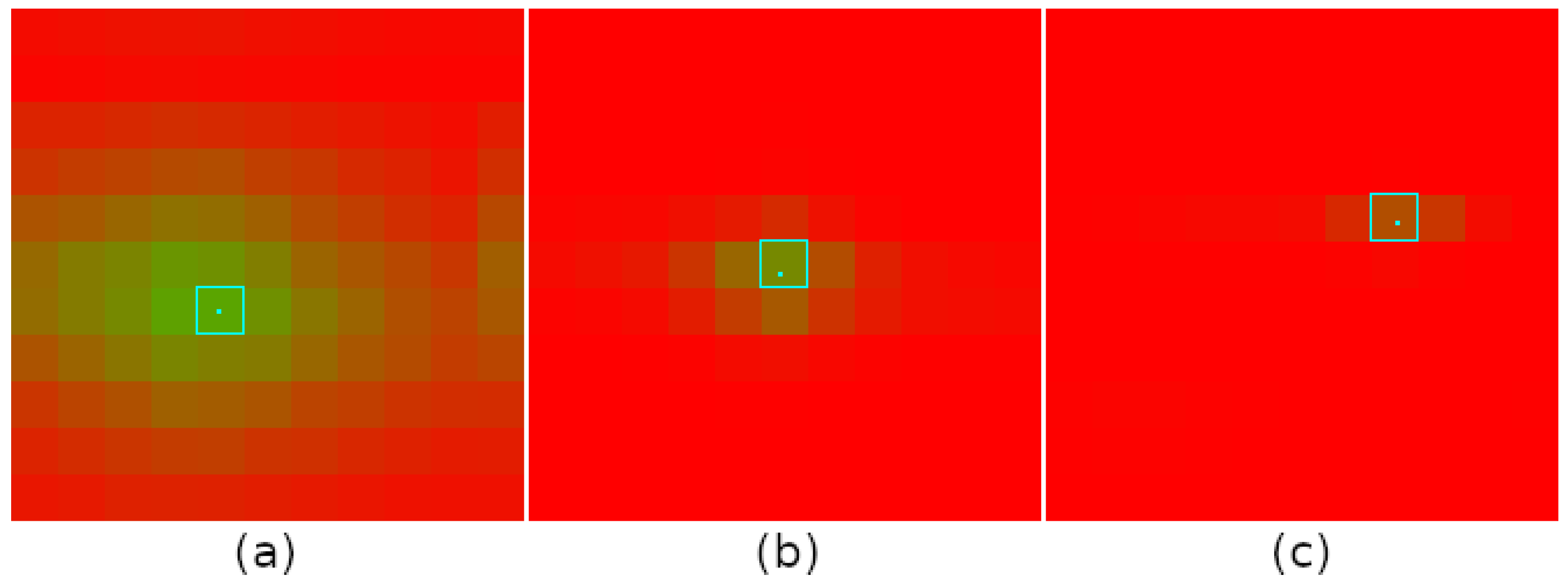
5.2. Effects of Grid Spacing

The spacing of grid cell modules may affect the precision of localization in the physical space i.e., the accuracy of visual odometry. A module with a smaller spacing will allow estimating the position and orientation of the agent in a smaller area around the active place cell, but with higher accuracy.

To evaluate the effect of grid spacing on precision and sensitivity to noise, we tested the navigation model with different grid cell spacings, from 0.1 to 1 BU (Figure 9). We observed that with a very short spacing (0.1 BU), a large amount of grid cells were active, with very little difference in the activity level between adjacent grid cells, making the module very sensitive to noise (e.g., from image data). As a result, detecting when the agent reached border grid cells became very inaccurate and less reliable. With a large spacing (>0.7 BU), very few grid cells are simultaneously active as each grid cell maps a greater area which decreases the precision of the estimated position. Moreover, because of the greater module coverage, we observed more inaccuracies in place cell’s context updates, leading to a lower precision in visual odometry.

The collected results show that a spacing of 0.3 BU offers a good compromise between precision and robustness to noise. For this reason, we use this spacing value in the subsequent experiments.

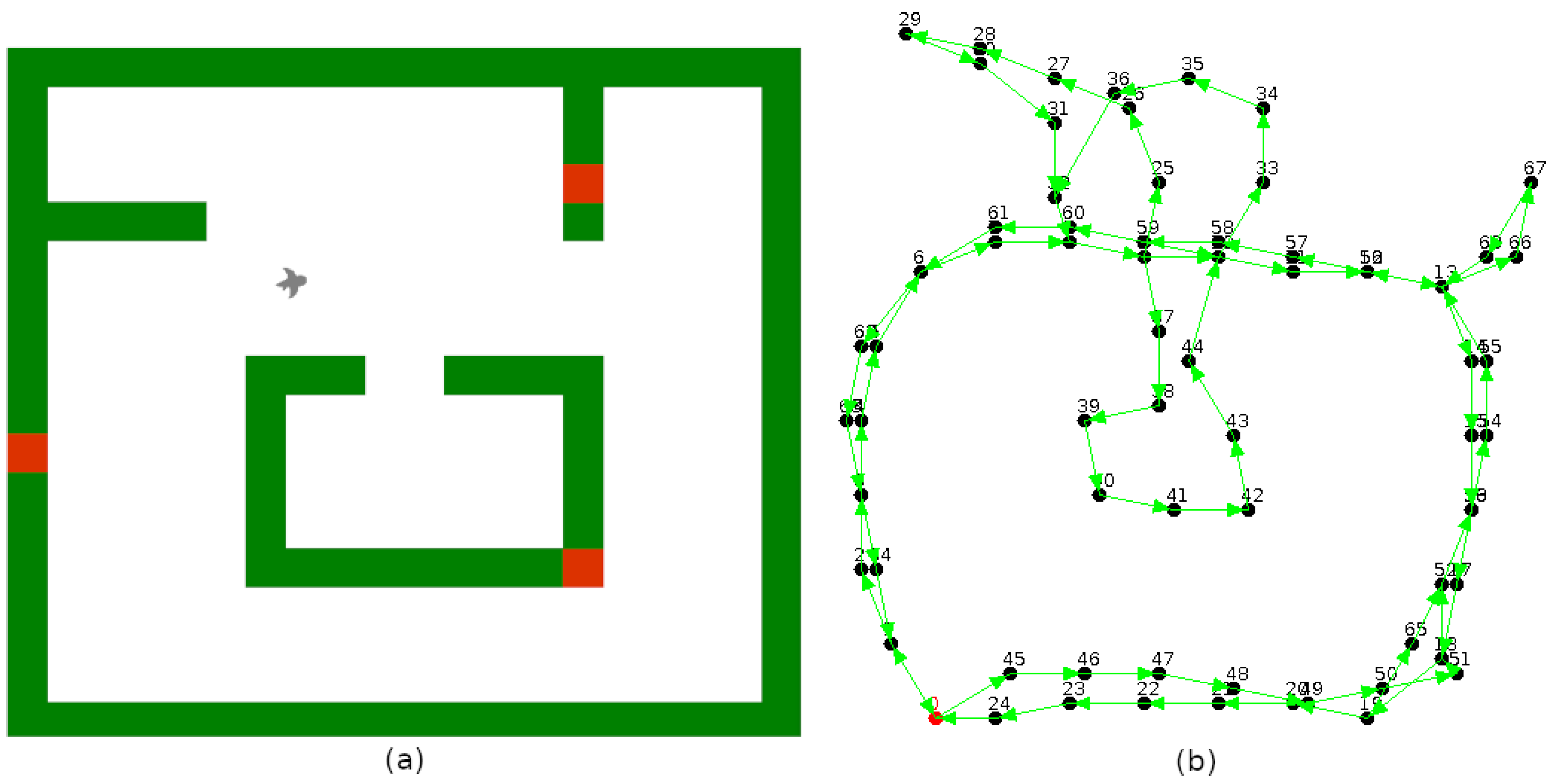
5.3. Navigation Graph Construction: Place Recognition

The goal of this test is to evaluate the drift of the estimated position in relation to the ground truth when exploring a new environment, and to show that known locations are recognized. The graph construction is observed using a global grid that consists of the repeated grid module (Figure 10). Ground truth and estimated positions are updated by movement integration. The navigation system cannot access this representation. A path was defined using manual control mode. Although progressing in the environment, the navigation system tracks the position by adding new place cells.

Over five different runs, we observed an average error in position estimation compared to ground truth (yellow path in Figure 10) of 0.63 BU, with a maximum peak of 1.90 BU on one of the runs. After having completed the main environment loop, the first place cell reacts with a high activity, allowing the system to connect first and last place cell, thus closing the loop. At this connection point, we observed that the average error on the five runs is only 0.69 BU. Figure 10 shows a typical run with the estimated (blue path) and ground truth (yellow path) positions.

When moving back the reverse way, or moving in areas with too few visual cues, the system creates a new sequence of place cells. This makes the model able to compensate the lack of visual cues using the sequential nature of the constructed model, as suggested by biological observations [25]. Figure 11 shows the completed graph covering the environment proposed in Figure 8.

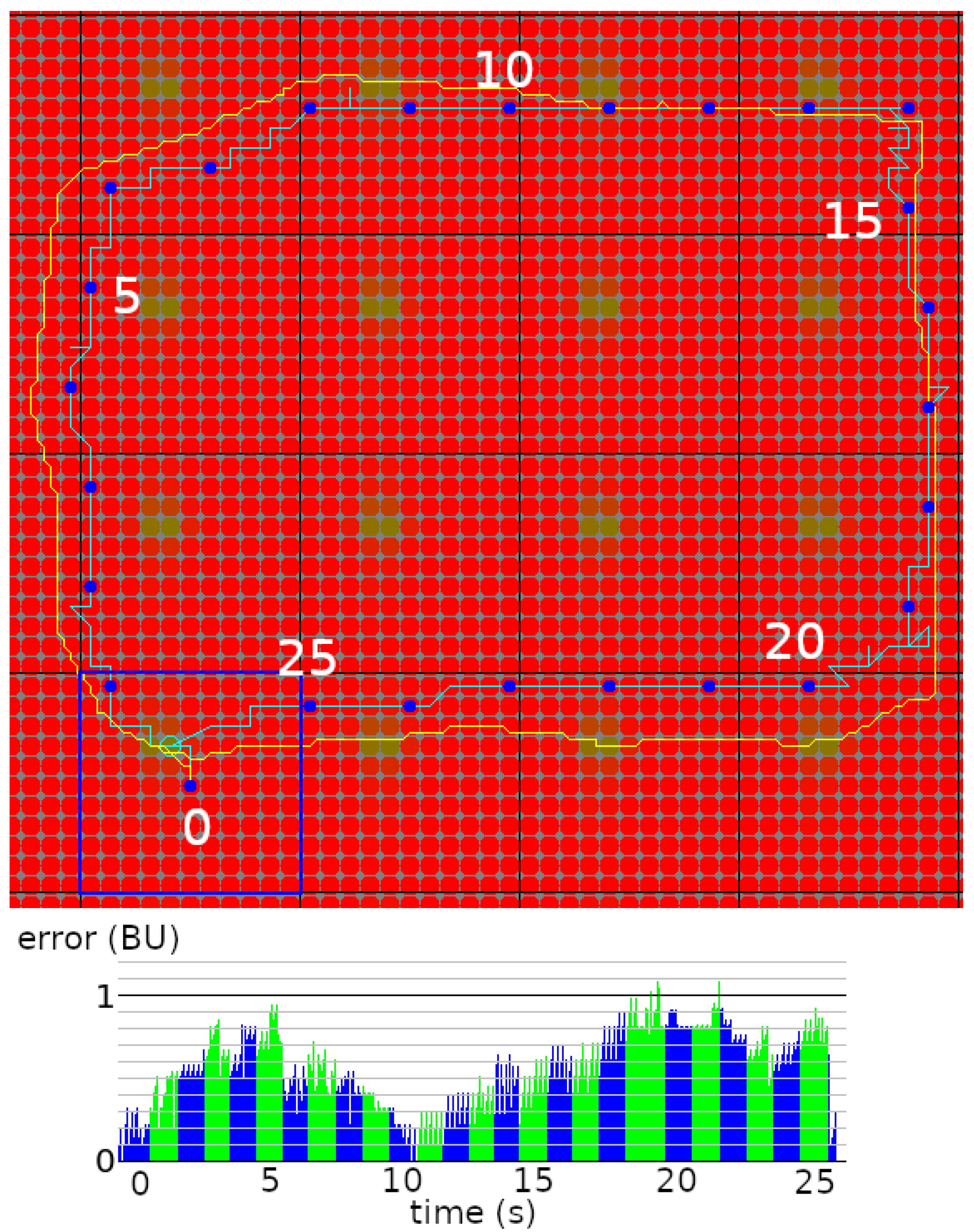
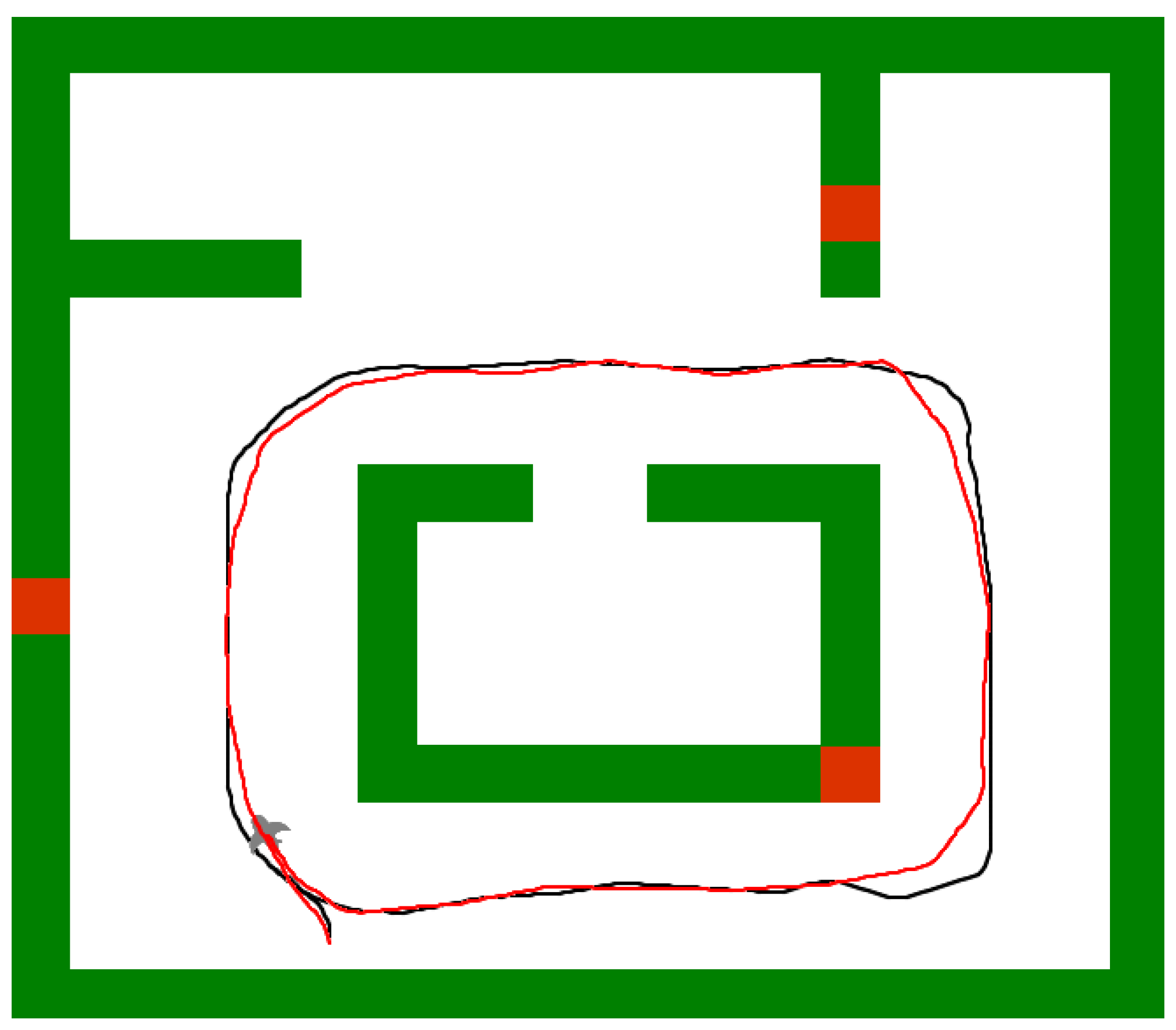
5.4. Usage of the Navigation Graph

We tested two navigation procedures in repeat mode: forward and backward, on a graph covering the main environment loop (Figure 8). Forward navigation follows a previously defined path in the same direction as it was created, while backward mode traces the path back to the starting point.

Forward navigation. Starting from the initial position (bottom left), the agent autonomously follows the path encoded by the sequence of place cells, by self-orienting towards the grid cell associated with the next place cell. The system sequentially loads contexts from place cells, allowing redefinition of its position and moving towards the next place cell. Figure 12 shows the trajectory successfully followed by the agent. The repeated path is thus very close to the original, although turns are a little tighter as the agent tries to move towards the next place cell in a straight line.

Backward navigation. Starting from the last place cell of the sequence, we activate the backward procedure. We observe the agent returns to its initial position, enacting the successive distances between place cells using only visual odometry. The navigation system generates a new sequence of place cells, as it cannot recognize first sequence. The trajectory is not as precise as in repeat mode, as the agent cannot re-estimate its position, although the final error between final and initial positions is of about several BU, depending on the first position (Figure 13).

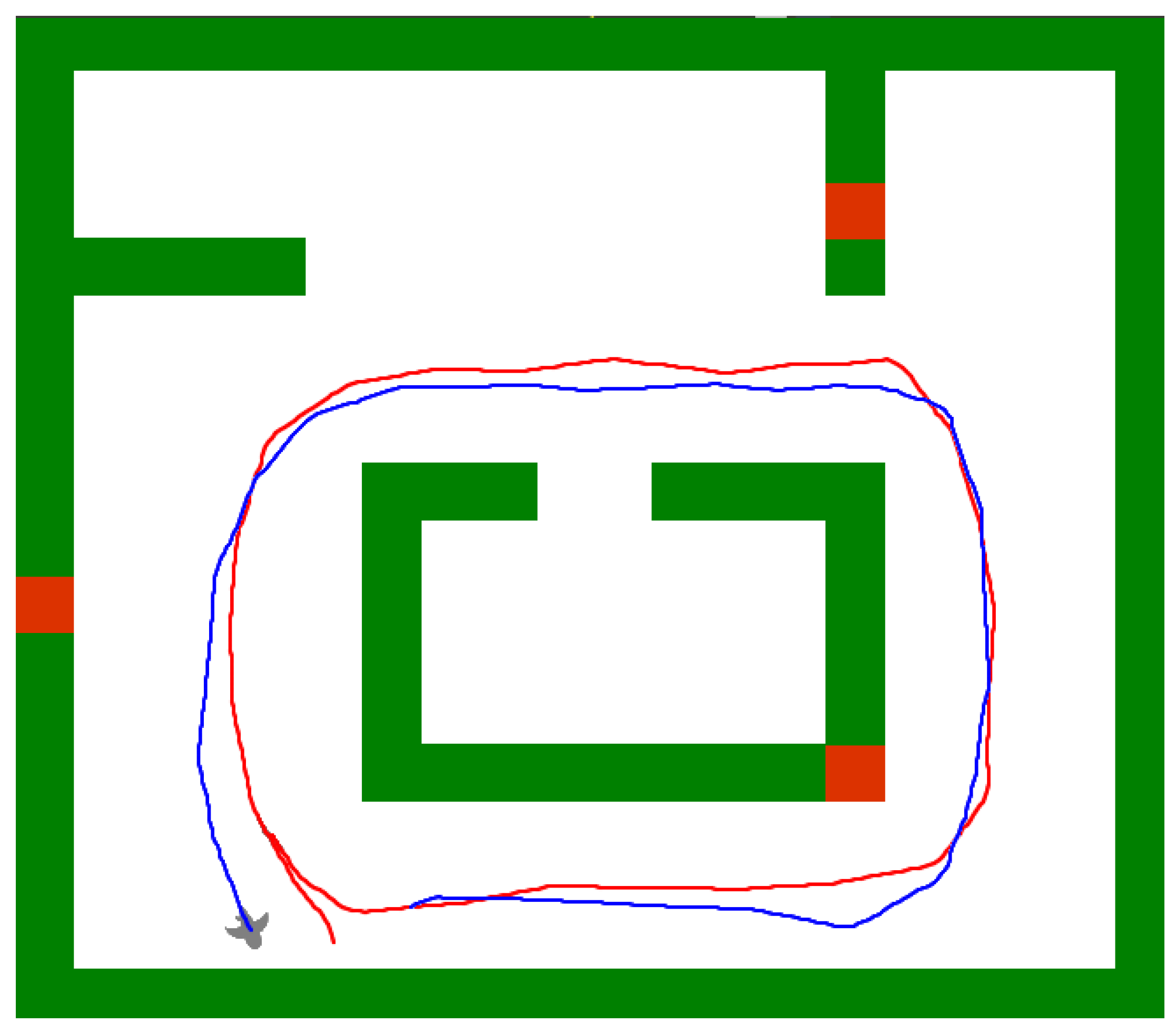
5.5. Robustness to Environmental Changes

Physical spaces are dynamic, their content and how they can be perceived change over time and with the viewpoint; for instance, opening and closing doors in buildings can cause the geometry of the environment to change. The robustness of the navigation model to changes in the environment was tested by modifying the content of the environment. Figure 14 provides an example of the modified initial environment (Figure 8). The place cell context update is deactivated to force the agent to use previously recorded contexts and avoid real-time updates; the repeat control mode to observe how the agent behaves.

Despite significant changes in the environment, the agent can still move through the sequence of place cells and successfully repeat the learned path. The trajectory remains close from the reference trajectory, as the system only considers cues that are close from predicted position. The path however deviates when cues are slightly moved, as they may interfere with other cues’ positions. The system fails when a large amount of cues, larger than remaining cues, are moved with the same offset.

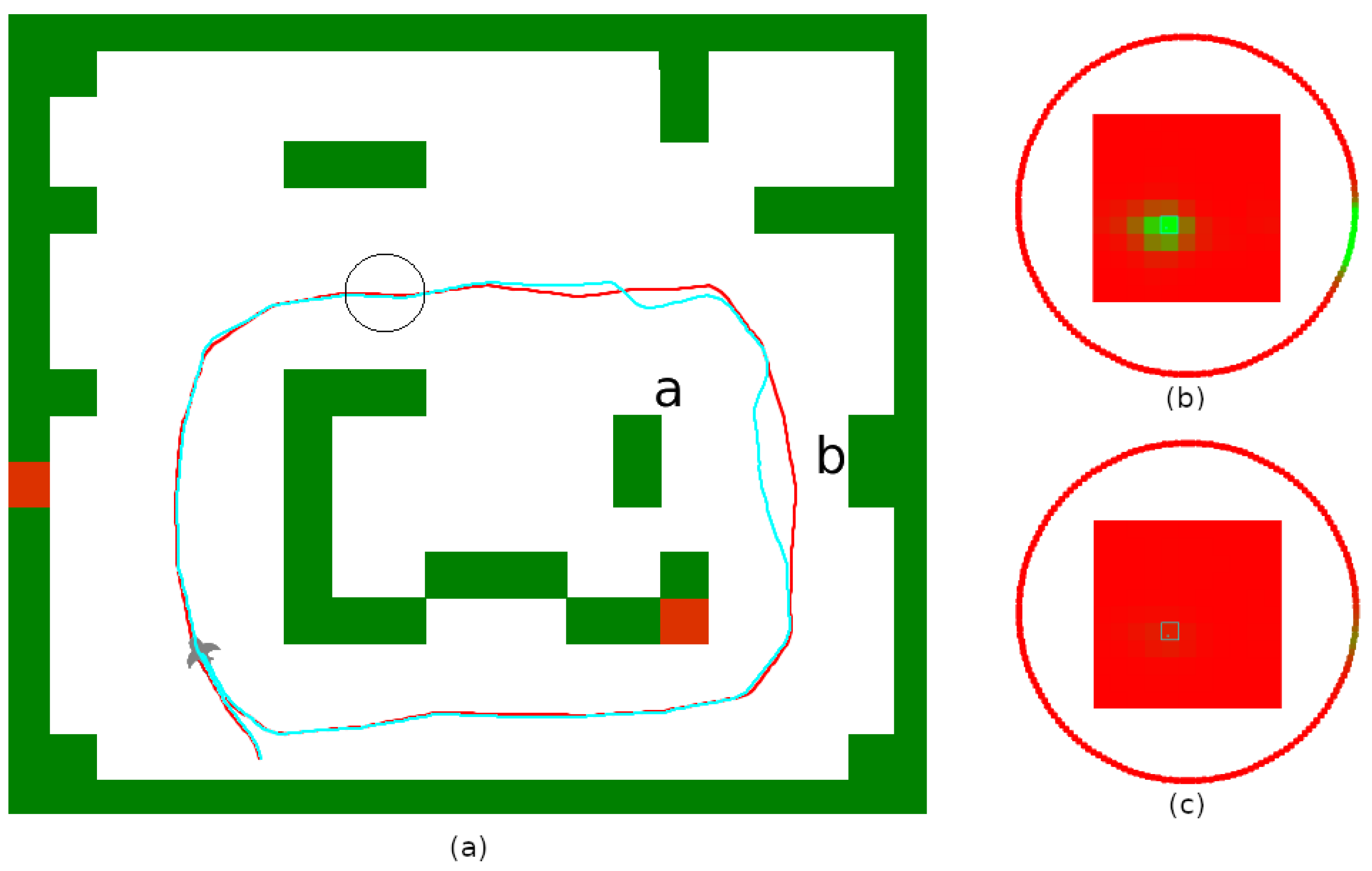
5.6. Finding Shortcuts

The shortcut finding mechanism was evaluated in repeat mode with a specifically modified initial environment. Figure 15 shows the tested environment and the obtained results. First and last place cells of the main loop were disconnected, and the agent starts from the third place cell’s position, preventing it from observing the last place cell and moving directly towards it. We removed several blocks on the south wall to open a shortcut in the environment.

The agent starts moving towards the visible place cell that is the closest from the last place cell in the sequence, which is a place cell close to north-west corner. When moving horizontally in the northern part of the environment, the agent can see an empty space covering place cells that are close to the last place cell of the sequence on its right (associated with positions on the south of the environment), and moves towards them. The agent then moves towards the estimated position of those place cells, creating a new sequence of place cell to track its position and updating the estimated position of the targeted place cell. Then, the agent enters the south corridor, recognizes the environment and connects the shortcut sequence, before moving towards the last place cell of the sequence.

6. Conclusions and Discussion

This paper introduces a new approach to control the navigation of an agent (in known/unknown, indoor/outdoor environment) inspired by three types of mammalian navigation neurons, place, grid and head direction cells. This model can track the position of an artificial agent and provides with high reliability navigational data needed to reach a destination.

A simple visual system with limited field of view was used as input to test the robustness of the system’s visual odometry. Despite the low precision of visual inputs, low variety of visual environments, and the use of a unique grid cell module, the obtained results show that the tracking mechanism successfully estimates the position and orientation of the agent, thus confirming the correctness of the proposed model. The experiments on the basic navigational tasks show that the proposed model is able to construct a navigation graph and uses it successfully to follow a path and return to the starting position. The tests also showed the system is able to discover shortcuts and add them to the navigation graph.

This robustness comes from (1) the prediction-oriented estimations which make the system very tolerant to changes to the environment, (2) the use of interconnected local models of the environment with independent reference frames makes the system very tolerant to movement drifts and (3) the sequential nature of the system allowing it to compensate the lack of visual cues when estimating the position in the navigation graph. The constructed model of the environment can provide navigation data under the form of movements required to move through a path, making it very easy to exploit with higher level mechanisms.

Future works will focus on improving our model by:

• using multiple sensory inputs. The use of inertial data (e.g., IMU) will increase the tracking reliability and enable navigation with few or no visual cues. Other sensory modalities, such as touch and audio, could help to complete a context.
• improving the place cell graph management, with mechanisms to split or merge place cells to avoid redundancies and correct observed errors (drift).
• using multiple grid cell modules with different orientations and spacings to increase the accuracy and reliability of localization. Following the approach proposed by Banino et al. [26] and Sparse Distributed Representations [27], associating a place cell with grid cells from different modules will help define a more unique position in space, as their combined activation will be sparser, which will increase the reliability of a place cell’s recognition.
• testing our model on physical devices. In a preliminary work, we successfully tested a grid cell module with a stereo camera. We intend to make our model applicable to robotic platforms, developmental agents, but also to assistive devices for people with visual impairments or spatial neglect. This last use case implies that our model can work with embedded cameras of limited field of view (we intend to use a stereo camera worn on the chest of the user), which can move in any direction, and cannot rely on absolute odometry (e.g., wheel encoders).

Moreover, this model shares very similar properties with the space memory architecture [21], suggesting that our navigation mechanism could be combined with it, using affordances instead of visual cues, to extend behavioral possibilities of developmental agents. In this developmental perspective, it would be interesting to study how movements associated with grid cells and head direction cells could be learned from the interactions between the agent and the environment.

References

1. López, E.; García, S.; Barea, R.; Bergasa, L.; Molinos, E.; Arroyo, R.; Romera, E.; Pardo, S. A Multi-Sensorial Simultaneous Localization and Mapping (SLAM) System for Low-Cost Micro Aerial Vehicles in GPS-Denied Environments. Sensors 2017, 17, 802. [Google Scholar] [CrossRef] [PubMed]
2. Stasse, O. SLAM and Vision-based Humanoid Navigation. In Humanoid Robotics: A Reference; HAL: Lyon, France, 2018; pp. 1739–1761. [Google Scholar] [CrossRef] [Green Version]
3. Cadena, C.; Carlone, L.; Carrillo, H.; Latif, Y.; Scaramuzza, D.; Neira, J.; Reid, I.; Leonard, J.J. Past, Present, and Future of Simultaneous Localization And Mapping: Towards the Robust-Perception Age. IEEE Trans. Robot. 2016, 32, 1309–1332. [Google Scholar] [CrossRef] [Green Version]
4. O’Keefe, J.; Nadel, L. The Hippocampus as a Cognitive Map; Clarendon Press: Oxford, UK, 1978. [Google Scholar]
5. Taube, J.; Muller, R.; Ranck, J. Head-Direction Cells Recorded from the Postsubiculum in Freely Moving Rats. I. Description and Quantitative Analysis. J. Neurosci. 1990, 10, 420. [Google Scholar] [CrossRef] [PubMed] [Green Version]
6. Rivière, M.A.; Gay, S.; Pissaloux, E. TactiBelt: Integrating Spatial Cognition and Mobility Theories into the Design of a Novel Orientation and Mobility Assistive Device for the Blind. In Computers Helping People with Special Needs; Lecture Notes in Computer Science; Miesenberger, K., Kouroupetroglou, G., Eds.; Springer: Berlin, Germany, 2018; Volume 10897, pp. 110–113. [Google Scholar] [CrossRef]
7. Li, K.; Malhotra, P.A. Spatial neglect. Pract. Neurol. 2015, 15, 333–339. [Google Scholar] [CrossRef] [PubMed] [Green Version]
8. Bainbridge, W.A.; Pounder, Z.; Eardley, A.F.; Baker, C.I. Quantifying Aphantasia through drawing: Those without visual imagery show deficits in object but not spatial memory. bioRxiv 2020. [Google Scholar] [CrossRef]
9. Hafting, T.; Fyhn, M.; Molden, S.; Moser, M.B.; Moser, E.I. Microstructure of a spatial map in the entorhinal cortex. Nature 2005, 436, 801–806. [Google Scholar] [CrossRef] [PubMed]
10. Gaussier, P.; Banquet, J.P.; Cuperlier, N.; Quoy, M.; Aubin, L.; Jacob, P.Y.; Sargolini, F.; Save, E.; Krichmar, J.L.; Poucet, B. Merging information in the entorhinal cortex: What can we learn from robotics experiments and modeling? J. Exp. Biol. 2019, 222, jeb186932. [Google Scholar] [CrossRef] [PubMed] [Green Version]
11. Jauffret, A.; Cuperlier, N.; Gaussier, P. From grid cells and visual place cells to multimodal place cell: A new robotic architecture. Front. Neurorobotics 2015, 9. [Google Scholar] [CrossRef] [PubMed]
12. Zhou, X.; Weber, C.; Wermter, S. A Self-organizing Method for Robot Navigation based on Learned Place and Head-Direction Cells. In Proceedings of the 2018 International Joint Conference on Neural Networks (IJCNN), Rio de Janeiro, Brazil, 8–13 July 2018; pp. 1–8. [Google Scholar] [CrossRef]
13. Zhou, X.; Bai, T.; Gao, Y.; Han, Y. Vision-Based Robot Navigation through Combining Unsupervised Learning and Hierarchical Reinforcement Learning. Sensors 2019, 19, 1576. [Google Scholar] [CrossRef] [PubMed] [Green Version]
14. Chen, Q.; Mo, H. A Brain-Inspired Goal-Oriented Robot Navigation System. Appl. Sci. 2019, 9, 4869. [Google Scholar] [CrossRef] [Green Version]
15. Karaouzene, A.; Delarboulas, P.; Vidal, D.; Gaussier, P.; Quoy, M.; Ramesh, C. Social interaction for object recognition and tracking. In Proceedings of the IEEE ROMAN Workshop on Developmental and Bio-Inspired Approaches for Social Cognitive Robotics, Coimbra, Portugal, 18–22 March 2013. [Google Scholar]
16. Milford, M.; Wyeth, G. Persistent Navigation and Mapping using a Biologically Inspired SLAM System. Int. J. Robot. Res. 2010, 29, 1131–1153. [Google Scholar] [CrossRef]
17. Milford, M.J.; Wyeth, G.F. SeqSLAM: Visual route-based navigation for sunny summer days and stormy winter nights. In Proceedings of the 2012 IEEE International Conference on Robotics and Automation, Saint Paul, MN, USA, 14–18 May 2012; pp. 1643–1649. [Google Scholar] [CrossRef]
18. Tang, H.; Yan, R.; Tan, K.C. Cognitive Navigation by Neuro-Inspired Localization, Mapping, and Episodic Memory. IEEE Trans. Cogn. Dev. Syst. 2018, 10, 751–761. [Google Scholar] [CrossRef]
19. O’Regan, J.K.; Noë, A. What it is like to see: A sensorimotor theory of perceptual experience. Synthese 2001, 129, 79–103. [Google Scholar] [CrossRef]
20. Georgeon, O.L.; Aha, D. The Radical Interactionism Conceptual Commitment. J. Artif. Gen. Intell. 2013, 4, 31–36. [Google Scholar]
21. Gay, S.L.; Mille, A.; Georgeon, O.L.; Dutech, A. Autonomous construction and exploitation of a spatial memory by a self-motivated agent. Cogn. Syst. Res. 2017, 41, 1–35. [Google Scholar] [CrossRef]
22. Grieves, R.M.; Jeffery, K.J. The representation of space in the brain. Behav. Process. 2017, 135, 113–131. [Google Scholar] [CrossRef] [PubMed]
23. Gay, S.L.; Mille, A.; Cordier, A. Autonomous affordance construction without planning for environment-agnostic agents. In Proceedings of the 2016 Joint IEEE International Conference on Development and Learning and Epigenetic Robotics (ICDL-EpiRob), Cergy-Pontoise, France, 19–22 September 2016; pp. 111–116. [Google Scholar] [CrossRef] [Green Version]
24. Stensola, H.; Stensola, T.; Solstad, T.; Frøland, K.; Moser, M.B.; Moser, E.I. The entorhinal grid map is discretized. Nature 2012, 492, 72–78. [Google Scholar] [CrossRef]
25. Wood, E.R.; Dudchenko, P.A.; Robitsek, R.; Eichenbaum, H. Hippocampal Neurons Encode Information about Different Types of Memory Episodes Occurring in the Same Location. Neuron 2000, 27, 623–633. [Google Scholar] [CrossRef] [Green Version]
26. Banino, A.; Barry, C.; Uria, B.; Blundell, C.; Lillicrap, T.; Mirowski, P.; Pritzel, A.; Chadwick, M.J.; Degris, T.; Modayil, J.; et al. Vector-based navigation using grid-like representations in artificial agents. Nature 2018, 557, 429–433. [Google Scholar] [CrossRef] [PubMed]
27. Ahmad, S.; Hawkins, J. Properties of Sparse Distributed Representations and their Application to Hierarchical Temporal Memory. arXiv 2015, arXiv:1503.07469. [Google Scholar]
Figure 1. The activation field of a single grid cell (from [22]).
Information 12 00100 g001
Figure 2. Graph of place cells associated with navigation in a physical space (pink node: place cells with firing activity, blue nodes: inactive place cells. Active place cell is designated with a green circle).
Information 12 00100 g002
Figure 3. Cooperation of “brain substrates” while predicting movement in the space: the active place cell (top, pink) is associated with one grid cell in each module (middle). The couple of grid cell and head direction cell (middle, green and bottom, green) give an estimate of the movement around the active place cell.
Information 12 00100 g003
Figure 4. The context in the agent’s egocentric reference frame: the orange triangle is the agent, colored dots are visual cues. The elements in the current context are given in polar coordinates.
Information 12 00100 g004
Figure 5. Head direction cells cover the [ 0 ; 2 π ] interval uniformly. The head direction cells use the current context observed by the agent as input and rotates this context by their attributed angle. Each head direction cell thus simulates a different rotation of the agent from its current orientation. These rotated contexts are then used in combination with contexts produced by grid cells to estimate the orientation of the agent (see Section 4.4 and Equation (2)).
Information 12 00100 g005
Figure 6. Principle of grid cell localization and odometry: a place cell is associated with a grid cell of a module. When the place cell becomes active (a), grid cells of the module generate alternatives of the place cell’s context, translated by the relative movement between each grid cell of the module and the grid cell associated with the place cell (b). The activity of grid cells in the module allows estimation of the agent’s current position and movements in the place cell’s reference (c).
Information 12 00100 g006
Figure 7. Generation of a new place cell: the center of the grid module defines a set of grid cells as border grid cells. When reaching a border grid cell, a new place cell is added, and associated with this border grid cell, which then becomes the new center of this module.
Information 12 00100 g007
Figure 8. Experimental environment used: (a) the test environment is populated with green blocks and several red blocks to help discriminate similar places. (b) the agent’s 180 visual field (the agent can only use polar coordinates), which depth estimation precision decreases with distance. Inner corners, outer corners, and color changes are detected (respectively yellow, cyan and magenta circles). (c) the agent’s visual context is also given in a Cartesian reference frame (used to simplify grid cell module context computation). The agent is indicated in blue in figures (b,c), its field of view is egocentric.
Information 12 00100 g008
Figure 9. Grid cell module with a spacing of 0.1 (a), 0.3 (b) and 0.9 BU (c) (chosen within the considered variations of grid spacing [ 0.1 ; 1 ] ), in the context given in Figure 8. With a low spacing (a), estimated position is very sensitive to noise. With a larger spacing (c), the precision of the estimated position drops as a grid cell represents a larger area.
Information 12 00100 g009
Figure 10. Top: example of tracking when traveling through the main environment loop (Figure 8). Yellow line indicates ground truth, cyan line indicates estimated position. Place cells are represented with blue points, displaying the associated grid cell (note that the grid cell module is repeated). Bottom: estimated position error through time, in Block Unit (BU). Color changes indicate place cell changes.
Information 12 00100 g010
Figure 11. (a) the environment in which the test was conducted. (b) navigation graph obtained after covering the whole environment. The distances between place cells are computed in the grid cell module space, which do not exactly match physical distances.
Information 12 00100 g011
Figure 12. Forward navigation: the agent autonomously follows the path given by a sequence of place cell starting in the bottom left. The autonomous trajectory (red) is very close to the manual trajectory (black).
Information 12 00100 g012
Figure 13. Backward navigation: the agent follows the path backwards to return to its starting position (blue trajectory), using only visual odometry and relative distance between place cells. The path is however not very precise due to the motion drift that is not corrected.
Information 12 00100 g013
Figure 14. Robustness to environmental changes: (a) repeat mode in a modified environment. Despite the environment changes, the trajectory (cyan) remains close from the one in the initial environment (red). We observe that corner (a) and wall (b), which were moved but are still close to original position, disrupt the position estimation in the grid cell module, causing deviations in the trajectory. Figures (b,c) show the grid cells (square) and head direction cells (circle) activity in (b) reference and (c) modified environments at the position marked with a circle: despite a very weak activity, the cells can still estimate the correct position and orientation.
Information 12 00100 g014
Figure 15. Forward navigation with shortcut finding system. First and last place cell are disconnected. The agent moves towards the most distant place cell that it can observe, and when it passes close to the shortcut, it observes a place cell that is very close from the destination place cell, and turns to take the shortcut. The agent then creates a new sequence of place cell until it reaches the destination place cell.
Information 12 00100 g015
Publisher’s Note: MDPI stays neutral with regard to jurisdictional claims in published maps and institutional affiliations.