Short-Term Electricity Load Forecasting with Machine Learning


Abstract
1. Introduction
Literature Review
2. Materials and Methods
2.1. Data Sources, Data Extraction, and Data Preparation
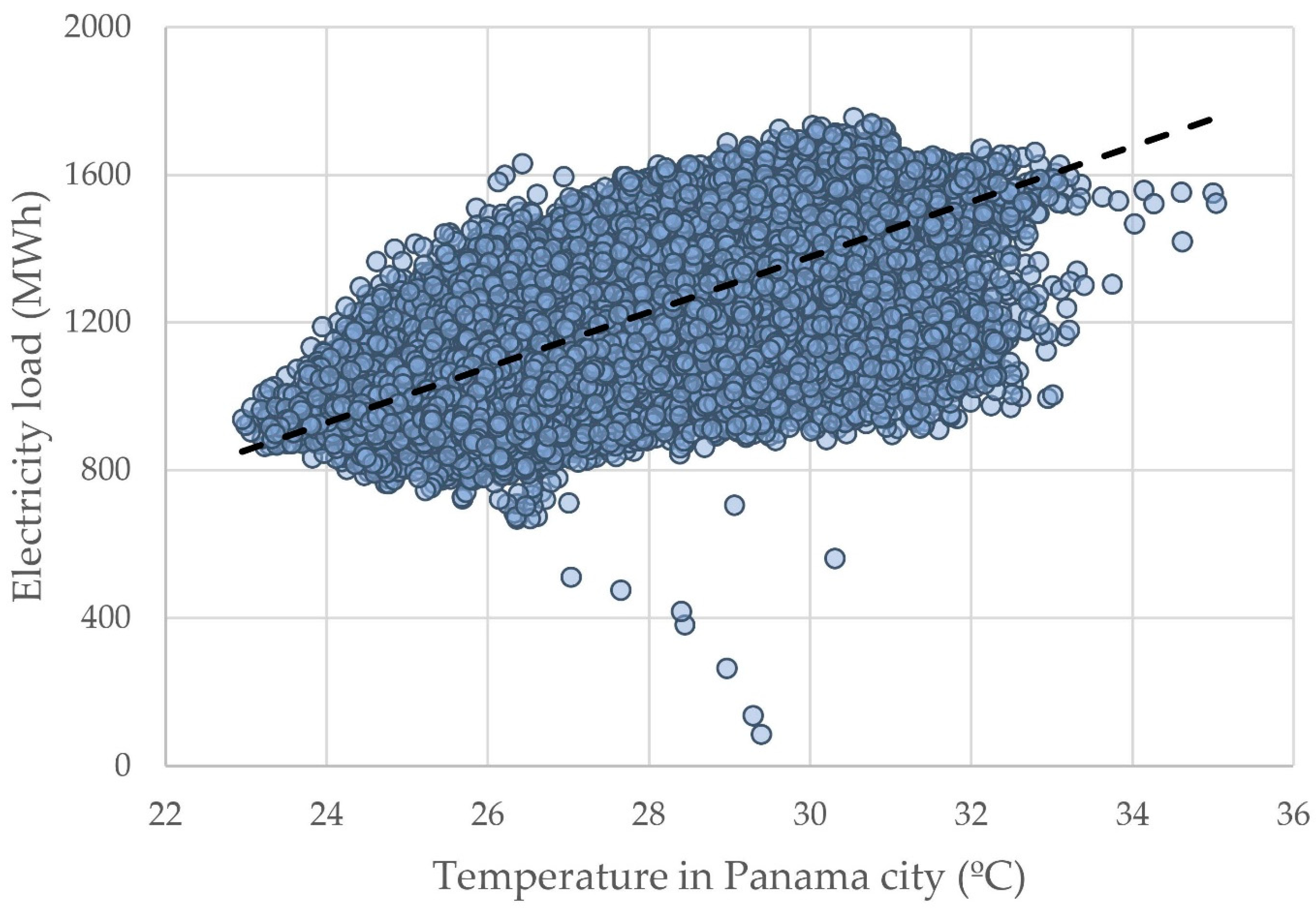
- Weather variables, such as temperature, relative humidity, precipitation, and wind speed, from three main cities in Panama, are gathered from EarthData satellite data [51].
2.2. Modeling
3. Results and Discussion
4. Conclusions
Limitations and Future Work
Author Contributions
Funding
Institutional Review Board Statement
Informed Consent Statement
Data Availability Statement
Conflicts of Interest
References
- Wood, A.J.; Wollenberg, B.; Sheblé, G. Power Generation, Operation, and Control, 3rd ed.; John Wiley & Sons: Hoboken, NJ, USA, 2013; pp. 63–302. [Google Scholar]
- Hossein, S.; Mohammad, S.S. Electric Power System Planning; Springer: Berlin/Heidelberg, Germany, 2011; p. 10. [Google Scholar]
- CND—ETESA, Metodologías de Detalle. Available online: https://www.cnd.com.pa/images/doc/norm_metodologiasdetalle_nov2020.pdf (accessed on 15 December 2020).
- PSR, NCP—Short Term Operation Programming. Available online: https://www.psr-inc.com/softwares-en/?current=p4034 (accessed on 4 November 2020).
- ABB HITACHI, Nostradamus. Available online: https://www.hitachiabb-powergrids.com/latam/es/offering/product-and-system/enterprise/energy-portfolio-management/trading-and-risk-management/nostradamus (accessed on 30 December 2020).
- CND—ETESA, Sistema de Información en Tiempo Real (SITR). Available online: http://sitr.cnd.com.pa/m/pub/sin.html (accessed on 2 September 2020).
- Aguilar, M.E.; Valdés, B.L. Impacto de La Entrada de La Generación Eólica y Fotovoltaica en Panamá. I+D Tecnológico. 2017, 13, 71–82. Available online: https://revistas.utp.ac.pa/index.php/id-tecnologico/article/view/1440 (accessed on 6 December 2020).
- Morales-Espana, G.; Latorre, J.M.; Ramos, A. Tight and Compact MILP Formulation of Start-Up and Shut-Down Ramping in Unit Commitment. IEEE Trans. Power Syst. 2012, 28, 1288–1296. [Google Scholar] [CrossRef]
- Becirovic, E.; Cosovic, M. Machine learning techniques for short-term load forecasting. In Proceedings of the 2016 4th International Symposium on Environmental Friendly Energies and Applications (EFEA), Belgrade, Serbia, 14–16 September 2016; pp. 1–4. [Google Scholar] [CrossRef]
- Li, C. Designing a short-term load forecasting model in the urban smart grid system. Appl. Energy 2020, 266, 114850. [Google Scholar] [CrossRef]
- Fernandes, R.S.S.; Bichpuriya, Y.K.; Rao, M.S.S.; Soman, S.A. Day ahead load forecasting models for holidays in Indian context. In Proceedings of the 2011 International Conference on Power and Energy Systems, Las Vegas, NV, USA, 12–14 November 2012. [Google Scholar] [CrossRef]
- Sarmiento, H.O.; Valencia, J.A.; Villa, W. Load forecasting with Neural Networks for Antioquia-Choco region. In Proceedings of the 2010 IEEE/PES Transmission and Distribution Conference and Exposition: Latin America (T&D-LA), Sao Paulo, Brazil, 8–10 November 2008; pp. 1–7. [Google Scholar] [CrossRef]
- Adeoye, O.; Spataru, C. Modelling and forecasting hourly electricity demand in West African countries. Appl. Energy 2019, 242, 311–333. [Google Scholar] [CrossRef]
- Dietrich, B.; Walther, J.; Weigold, M.; Abele, E. Machine learning based very short term load forecasting of machine tools. Appl. Energy 2020, 276, 115440. [Google Scholar] [CrossRef]
- Lebotsa, M.E.; Sigauke, C.; Bere, A.; Fildes, R.; Boylan, J.E. Short term electricity demand forecasting using partially linear additive quantile regression with an application to the unit commitment problem. Appl. Energy 2018, 222, 104–118. [Google Scholar] [CrossRef]
- Zhu, K.; Geng, J.; Wang, K. A hybrid prediction model based on pattern sequence-based matching method and extreme gradient boosting for holiday load forecasting. Electr. Power Syst. Res. 2021, 190, 106841. [Google Scholar] [CrossRef]
- Ferreira, P.M.; Cuambe, I.D.; Ruano, A.; Pestana, R. Forecasting the Portuguese Electricity Consumption using Least-Squares Support Vector Machines. IFAC Proc. Vol. 2013, 46, 411–416. [Google Scholar] [CrossRef]
- Zou, M.; Fang, D.; Harrison, G.; Djokic, S. Weather Based Day-Ahead and Week-Ahead Load Forecasting using Deep Recurrent Neural Network. In 2019 IEEE 5th International forum on Research and Technology for Society and Industry (RTSI); Institute of Electrical and Electronics Engineers (IEEE): Piscataway, NJ, USA, 2019; pp. 341–346. [Google Scholar]
- Dutta, S.; Li, Y.; Venkataraman, A.; Costa, L.M.; Jiang, T.; Plana, R.; Tordjman, P.; Choo, F.H.; Foo, C.F.; Puttgen, H.B. Load and Renewable Energy Forecasting for a Microgrid using Persistence Technique. Energy Procedia 2017, 143, 617–622. [Google Scholar] [CrossRef]
- Paterakis, N.; Mocanu, E.; Gibescu, M.; Stappers, B.; Van Alst, W. Deep learning versus traditional machine learning methods for aggregated energy demand prediction. In 2017 IEEE PES Innovative Smart Grid Technologies Conference Europe (ISGT-Europe); Institute of Electrical and Electronics Engineers (IEEE): Piscataway, NJ, USA, 2017; pp. 1–6. [Google Scholar]
- Barakat, E.H.; Al-Qasem, J.M. Methodology for weekly load forecasting. IEEE Trans. Power Syst. 1998, 13, 1548–1555. [Google Scholar] [CrossRef]
- Amjady, N. Short-term hourly load forecasting using time-series modeling with peak load estimation capability. IEEE Trans. Power Syst. 2001, 16, 798–805. [Google Scholar] [CrossRef]
- Al-Musaylh, M.S.; Deo, R.C.; Adamowski, J.; Li, Y. Short-term electricity demand forecasting with MARS, SVR and ARIMA models using aggregated demand data in Queensland, Australia. Adv. Eng. Inform. 2018, 35, 1–16. [Google Scholar] [CrossRef]
- Al Amin, M.A.; Hoque, M.A. Comparison of ARIMA and SVM for short-term load forecasting. In Proceedings of the IEMECON 2019-9th Annual Information Technology Electromechanical Eng. Microelectron Conference, Lisbon, Portugal, 14–17 October 2019; pp. 205–210. [Google Scholar]
- Chapagain, K.; Kittipiyakul, S. Short-Term Electricity Demand Forecasting with Seasonal and Interactions of Variables for Thailand. In Proceedings of the 2018 International Electrical Engineering Congress (iEECON), Krabi, Thailand, 7–9 March 2018. [Google Scholar] [CrossRef]
- Liu, F.; Findlay, R.D.; Song, Q. A Neural Network Based Short Term Electric Load Forecasting in Ontario Canada. In Proceedings of the 2006 International Conference on Computational Inteligence for Modelling Control and Automation and International Conference on Intelligent Agents Web Technologies and International Commerce (CIMCA’06), Sydney, Australia, 9 November–1 December 2006; p. 119. [Google Scholar] [CrossRef]
- Ferreira, P.M.; Ruano, A.; Pestana, R. Improving the Identification of RBF Predictive Models to Forecast the Portuguese Electricity Consumption. IFAC Proc. Vol. 2010, 43, 208–213. [Google Scholar] [CrossRef]
- Omidi, A.; Barakati, S.M.; Tavakoli, S. Application of nusupport vector regression in short-term load forecasting. In 2015 20th Conference on Electrical Power Distribution Networks Conference (EPDC); Institute of Electrical and Electronics Engineers (IEEE): New York, NY, USA, 2015; pp. 32–36. [Google Scholar]
- Pinto, T.; Praça, I.; Vale, Z.; Silva, J. Ensemble learning for electricity consumption forecasting in office buildings. Neurocomputing 2021, 423, 747–755. [Google Scholar] [CrossRef]
- Hadri, S.; NaitMalek, Y.; Najib, M.; Bakhouya, M.; Fakhri, Y.; El Aroussi, M. A Comparative Study of Predictive Approaches for Load Forecasting in Smart Buildings. Procedia Comput. Sci. 2019, 160, 173–180. [Google Scholar] [CrossRef]
- Cai, J.; Cai, H.; Cai, Y.; Wu, L.; Shen, Y. Short-term Forecasting of User Power Load in China Based on XGBoost. In 2020 12th IEEE PES Asia-Pacific Power and Energy Engineering Conference (APPEEC); Institute of Electrical and Electronics Engineers (IEEE): New York, NY, USA, 2020; Volume 3, pp. 1–5. [Google Scholar]
- Suo, G.; Song, L.; Dou, Y.; Cui, Z. Multi-dimensional Short-Term Load Forecasting Based on XGBoost and Fireworks Algorithm. In Proceedings of the 2019 18th International Symposium on Distributed Computing and Applications for Business Engineering and Science (DCABES), Wuhan, China, 8–10 November 2019; pp. 245–248. [Google Scholar] [CrossRef]
- Liao, X.; Cao, N.; Li, M.; Kang, X. Research on Short-Term Load Forecasting Using XGBoost Based on Similar Days. In 2019 International Conference on Intelligent Transportation, Big Data & Smart City (ICITBS); Institute of Electrical and Electronics Engineers (IEEE): New York, NY, USA, 2019; pp. 675–678. [Google Scholar]
- Liu, Y.; Luo, H.; Zhao, B.; Zhao, X.; Han, Z. Short-Term Power Load Forecasting Based on Clustering and XGBoost Method. In 2018 IEEE 9th International Conference on Software Engineering and Service Science (ICSESS); Institute of Electrical and Electronics Engineers (IEEE): New York, NY, USA, 2018; pp. 536–539. [Google Scholar]
- Zheng, H.; Yuan, J.; Chen, L. Short-Term Load Forecasting Using EMD-LSTM Neural Networks with a Xgboost Algorithm for Feature Importance Evaluation. Energies 2017, 10, 1168. [Google Scholar] [CrossRef]
- Xue, P.; Jiang, Y.; Zhou, Z.; Chen, X.; Fang, X.; Liu, J. Multi-step ahead forecasting of heat load in district heating systems using machine learning algorithms. Energy 2019, 188, 116085. [Google Scholar] [CrossRef]
- Yu, X.; Wang, Y.; Wu, L.; Chen, G.; Wang, L.; Qin, H. Comparison of support vector regression and extreme gradient boosting for decomposition-based data-driven 10-day streamflow forecasting. J. Hydrol. 2020, 582, 124293. [Google Scholar] [CrossRef]
- Khwaja, A.S.; Anpalagan, A.; Naeem, M.; Venkatesh, B. Joint bagged-boosted artificial neural networks: Using ensemble machine learning to improve short-term electricity load forecasting. Electr. Power Syst. Res. 2020, 179, 106080. [Google Scholar] [CrossRef]
- Singh, P.; Dwivedi, P. Integration of new evolutionary approach with artificial neural network for solving short term load forecast problem. Appl. Energy 2018, 217, 537–549. [Google Scholar] [CrossRef]
- Yan, G.; Han, T.; Zhang, W.; Zhao, S. Short-Term Load Forecasting of Smart Grid Based on Load Spatial-Temporal Distribution. In 2019 IEEE Innovative Smart Grid Technologies—Asia (ISGT Asia); Institute of Electrical and Electronics Engineers (IEEE): Piscataway, NJ, USA, 2019; pp. 781–785. [Google Scholar]
- Abbasimehr, H.; Shabani, M.; Yousefi, M. An optimized model using LSTM network for demand forecasting. Comput. Ind. Eng. 2020, 143, 106435. [Google Scholar] [CrossRef]
- Atef, S.; Eltawil, A.B. Assessment of stacked unidirectional and bidirectional long short-term memory networks for electricity load forecasting. Electr. Power Syst. Res. 2020, 187, 106489. [Google Scholar] [CrossRef]
- Vitynskyi, P.; Tkachenko, R.; Izonin, I.; Kutucu, H. Hybridization of the SGTM Neural-Like Structure Through Inputs Polynomial Extension. In 2018 IEEE Second International Conference on Data Stream Mining & Processing (DSMP); Institute of Electrical and Electronics Engineers (IEEE): New York, NY, USA, 2018; pp. 386–391. [Google Scholar]
- Google Colaboratory. Available online: https://research.google.com/colaboratory/faq.html (accessed on 19 November 2020).
- Guido, V.R.; Drake, F.L., Jr. Python 3 Reference Manual. Available online: https://docs.python.org/2/reference/lexical_analysis.html (accessed on 19 November 2020).
- CND—ETESA, Post-dispatch—Operating Reports. Available online: https://www.cnd.com.pa/index.php/informes/categoria/informes-de-operaciones?tipo=60 (accessed on 17 October 2020).
- CND—ETESA, Weekly pre-dispatch—Operating Reports. Available online: https://www.cnd.com.pa/index.php/informes/categoria/informes-de-operaciones?tipo=68&anio=2019&semana=0 (accessed on 17 October 2020).
- Gaceta Oficial—Ministerio de la Presidencia. Busqueda Avanzada. Available online: https://www.gacetaoficial.gob.pa/Busqueda-Avanzada (accessed on 19 November 2020).
- When on Earth? Calendar for Panama. Available online: https://www.whenonearth.com/calendar/panama/2020 (accessed on 19 November 2020).
- Goddard Earth Sciences Data and Information Services Center (GES DISC). Global Modeling and Assimilation Office (GMAO) (2015), MERRA-2 tavg1_2d_slv_Nx: 2d,1-Hourly, Time-Averaged, Single-Level, Assimilation, Single-Level Diagnostics V5.12.4, Greenbelt, MD, USA. Available online: https://disc.gsfc.nasa.gov/datasets/M2T1NXSLV_5.12.4/summary (accessed on 2 September 2020). [CrossRef]
- Wes McKinney and the Pandas Development Team. Pandas: Powerful Python Data Analysis Toolkit. Available online: https://pandas.pydata.org/docs/pandas.pdf (accessed on 6 December 2020).
- Nadh, K. netCDF4 API documentation. Available online: https://unidata.github.io/netcdf4-python/netCDF4/index.html (accessed on 19 November 2020).
- Hoyer, S.; Hamman, J.J. xarray: N-D labeled Arrays and Datasets in Python. J. Open Res. Softw. 2017, 5, 10. [Google Scholar] [CrossRef]
- Zhang, N.; Li, Z.; Zou, X.; Quiring, S.M. Comparison of three short-term load forecast models in Southern California. Energy 2019, 189, 116358. [Google Scholar] [CrossRef]
- Eseye, A.T.; Lehtonen, M.; Tukia, T.; Uimonen, S.; Millar, R.J. Machine Learning Based Integrated Feature Selection Approach for Improved Electricity Demand Forecasting in Decentralized Energy Systems. IEEE Access 2019, 7, 91463–91475. [Google Scholar] [CrossRef]
- Han, J.; Kamber, M.; Pei, J. Data Reduction. In Data Mining, Concepts and Techniques, 3rd ed.; The Morgan Kaufmann Series; Data Management Systems: Waltham, MA, USA, 2011; pp. 99–110. [Google Scholar]
- Geéron, A. Hands-on Machine Learning with Scikit-Learn and Tensor Flow: Concepts, Tools, and Techniques to Build Intelligent Systems; O’Reilly Media: Sebastopol, CA, USA, 2017. [Google Scholar]
- Boya, C. Analyzing the Relationship between Temperature and Load Demand in the Regions with the Highest Electricity Consumption in the Republic of Panama. In 2019 7th International Engineering, Sciences and Technology Conference (IESTEC); Institute of Electrical and Electronics Engineers (IEEE): New York, NY, USA, 2019; pp. 132–137. [Google Scholar]
- La Estrella de Panamá. “Cuarentena en Panamá,” Calles Desiertas en el Primer día de Cuarentena Total en Panamá por COVID-19. Available online: https://www.laestrella.com.pa/nacional/200325/calles-desiertas-primer-dia-cuarentena-total-panama-covid-19 (accessed on 30 September 2020).
- Dietvorst, B.J.; Simmons, J.P.; Massey, C. Algorithm aversion: People erroneously avoid algorithms after seeing them err. J. Exp. Psychol. Gen. 2015, 144, 114–126. [Google Scholar] [CrossRef]
- Bertsimas, D.; Delarue, A.; Jaillet, P.; Martin, S. The Price of Interpretability. 2019. Available online: https://arxiv.org/pdf/1907.03419.pdf (accessed on 21 November 2020).
- Pedregosa, F.; Varoquaux, G.; Gramfort, A.; Michel, V.; Thirion, B.; Grisel, O.; Blondel, M.; Prettenhofer, P; Weiss, R; Dubourg, V.; et al. Scikit-learn: Machine Learning in Python. J. Mach. Learn. Res. 2011, 39. Available online: https://jmlr.csail.mit.edu/papers/volume12/pedregosa11a/pedregosa11a.pdf (accessed on 10 December 2020).
- XGB Developers. XGBoost Documentation. Available online: https://xgboost.readthedocs.io/en/latest/ (accessed on 3 November 2020).
- Johannesen, N.J.; Kolhe, M.; Goodwin, M. Relative evaluation of regression tools for urban area electrical energy demand forecasting. J. Clean. Prod. 2019, 218, 555–564. [Google Scholar] [CrossRef]
- Alex, J.S.; Schölkopf, B. A Tutorial on Support Vector Regression. Stat. Comput. 2004, 14, 199–222. Available online: https://alex.smola.org/papers/2004/SmoSch04.pdf (accessed on 21 November 2020).
- Cao, L.; Li, Y.; Zhang, J.; Jiang, Y.; Han, Y.; Wei, J. Electrical load prediction of healthcare buildings through single and ensemble learning. Energy Rep. 2020, 6, 2751–2767. [Google Scholar] [CrossRef]
- Liu, X.; Zhang, Z.; Song, Z. A comparative study of the data-driven day-ahead hourly provincial load forecasting methods: From classical data mining to deep learning. Renew. Sustain. Energy Rev. 2020, 119, 109632. [Google Scholar] [CrossRef]
- Al Amin, M.A.; Hoque, A. Comparison of ARIMA and SVM for Short-term Load Forecasting. In 2019 9th Annual Information Technology, Electromechanical Engineering and Microelectronics Conference (IEMECON); Institute of Electrical and Electronics Engineers (IEEE): New York, NY, USA, 2019; pp. 1–6. [Google Scholar]
- Scikit-learn Developers. GradientBoostingRegressor. Available online: https://scikit-learn.org/stable/modules/generated/sklearn.ensemble.GradientBoostingRegressor.html (accessed on 21 November 2020).
- Time Series Data Prediction using Elman Recurrent Neural Network on Tourist Visits in Tanah Lot Tourism Object. Int. J. Eng. Adv. Technol. 2019, 9, 314–320. [CrossRef]
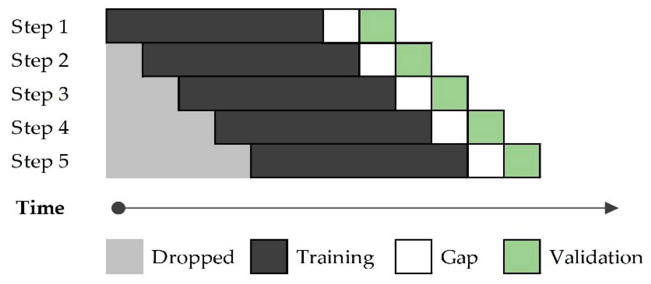
- Herman-Saffar, O. Time Based Cross Validation. Available online: https://towardsdatascience.com/time-based-cross-validation-d259b13d42b8 (accessed on 21 November 2020).
- Raschka, S. Feature Importance Permutation—mlxtend. Available online: http://rasbt.github.io/mlxtend/user_guide/evaluate/feature_importance_permutation/ (accessed on 2 December 2020).
- Massaoudi, M.; Refaat, S.S.; Chihi, I.; Trabelsi, M.; Oueslati, F.S.; Abu-Rub, H. A novel stacked generalization ensemble-based hybrid LGBM-XGB-MLP model for Short-Term Load Forecasting. Energy 2021, 214, 118874. [Google Scholar] [CrossRef]
- CND—ETESA. Informe de Planeamiento Operativo—Semestre I. 2020. Available online: https://sitioprivado.cnd.com.pa/Informe/Download/36121?key=VXd9e23Z9JRA5aIUR21R-P8gocoGOMqdvSo79FduN (accessed on 6 December 2020).
- CND—ETESA. Reglas Comerciales. Available online: https://www.cnd.com.pa/images/doc/norm_regcomerciales_enero2018.pdf (accessed on 1 December 2020).
- Visual Crossing. Historical Weather Data & Weather Forecast Data. Available online: https://www.visualcrossing.com/weather-data (accessed on 2 September 2020).
- Andersen, F.; Henningsen, G.; Møller, N.F.; Larsen, H.V. Long-term projections of the hourly electricity consumption in Danish municipalities. Energy 2019, 186, 115890. [Google Scholar] [CrossRef]
- Abbott, D. Applied Predictive Analytics. Principles and Techniques for the Professional Data Analyst; John Wiley & Sons, Inc.: Indianapolis, IN, USA, 2014; p. 372. [Google Scholar]


| Variable | Description | Unit of Measurement |
|---|---|---|
| National load | National electricity load, excluding exports | MWh |
| Holiday | Holiday binary indicator | - |
| School | School period binary indicator | - |
| Temp. 2 m c | Air temperature at 2 m | °C |
| Hum. 2 m c | Specific humidity at 2 m | % |
| Wind 2 m c | Wind speed at 2 m | m/s |
| Precipitation c | Total precipitable liquid water | l/m2 |
| Load Forecast | Historical national load forecast, excluding exports | MWh |
| Model | Hyperparameter | Randomized Search | RS 1 Selection | Grid Search | GS 2 Selection |
|---|---|---|---|---|---|
| KNN | n_neighbors | (3, 6, 9, 12, 15, 18, 21, 24, 27) | 29 | (23, 26, 29, 32, 35) | 29 |
| weights | (uniform, distance) | distance | (distance) | distance | |
| metric | (minkowski, euclidean, manhattan) | manhattan | (manhattan) | manhattan | |
| leaf_size | (5, 15, 25, 35) | 35 | (29, 32, 35, 38, 41) | 29 | |
| SVR | kernel | (linear, rbf) | rbf | (rbf) | rbf |
| epsilon | (0.0001, 0.3), step 0.01 | 0.0701 | (0.03505, 0.09113), step 0.01402 | 0.03505 | |
| C | (0.01, 0.1, 1, 10, 100) | 100 | (50, 70, 90, 110, 130) | 50 | |
| tol | (0.001) | 0.001 | (0.001) | 0.001 | |
| RF | criterion | (mse) | mse | (mse) | mse |
| n_estimators | (50, 100, 150, 200) | 200 | (200) | 200 | |
| max_samples | (0.5, 0.6, 0.7, 0.8, 0.9) | 0.5 | (0.5) | 0.5 | |
| max_depth | (10, 20, 30, 40, 50) | 40 | (20, 35, 50, 65) | 35 | |
| ccp_alpha | (5 × 10⁻⁷, 0.01), step 0.0005 | 0.0095005 | (0.0094, 0.0099, 0.0104, 0.0109, 0.0114) | 0.0094 | |
| random_state | (123) | 123 | (123) | 123 | |
| XGB | eval_metric | (rmse) | rmse | (rmse) | rmse |
| n_estimators | (100, 150, 200, 250, 300, 350, 400) | 300 | (300, 310, 320) | 300 | |
| max_depth | (3, 5) | 5 | (5, 7, 9) | 7 | |
| subsample | (0.6, 0.7, 0.8, 0.9) | 0.8 | (0.7) | 0.7 | |
| colsample_bytree | (0.7, 0.8, 0.9, 1.0) | 0.9 | (0.7, 0.75) | 0.7 | |
| colsample_bylevel | (0.7, 0.8, 0.9, 1.0) | 1.0 | (0.7) | 0.7 | |
| colsample_bynode | (0.7, 0.8, 0.9, 1.0) | 0.8 | (0.7, 0.75) | 0.7 | |
| learning_rate | (0.0001, 0.2501), step 0.05 | 0.0501 | (0.05, 0.045) | 0.045 | |
| min_child_weight | (1, 3, 5, 7) | 7 | (7) | 7 | |
| gamma | (0, 5, 10, 15) | 15 | (15) | 15.00 | |
| random_state | 123 | 123 | (123) | 123 |
| Metric | Definition | Equation | Unit |
|---|---|---|---|
| MAPE | mean absolute percent error | % | |
| RMSE | square root of mean square error | MWh | |
| Peak | peak load absolute percent error | % | |
| Valley | valley load absolute percent error | % | |
| Energy | energy absolute percent error | % |
| Model | Metric | Mean | SD | Min. | 25th Perc. | 50th Perc. | 75th Perc. | Max. |
|---|---|---|---|---|---|---|---|---|
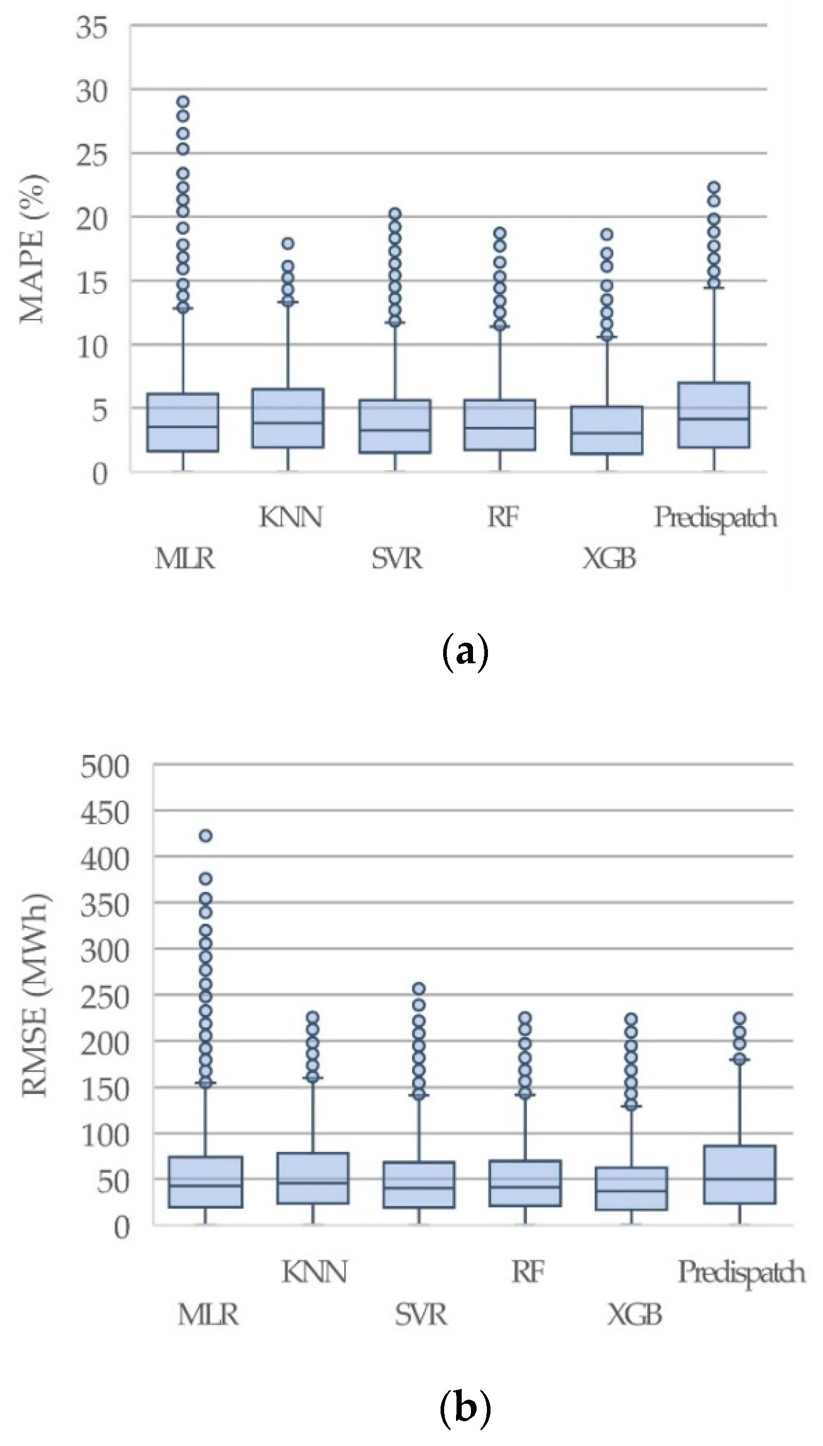
| Pre-Disp. | MAPE | 4.95 | 3.88 | 0.00 | 1.90 | 4.10 | 7.00 | 22.30 |
| RMSE | 59.20 | 44.45 | 0.00 | 23.13 | 49.50 | 85.80 | 224.60 | |
| Peak | 2.76 | 2.19 | 0.10 | 0.70 | 2.40 | 4.30 | 7.10 | |
| Valley | 4.48 | 3.02 | 0.30 | 2.10 | 4.15 | 5.90 | 11.90 | |
| Energy | 2.81 | 2.06 | 0.60 | 1.40 | 2.20 | 3.10 | 8.20 | |
| MLR | MAPE | 4.43 | 3.91 | 0.00 | 1.60 | 3.50 | 6.10 | 29.00 |
| RMSE | 53.97 | 49.66 | 0.00 | 19.40 | 42.45 | 73.45 | 431.40 | |
| Peak | 2.74 | 2.16 | 0.50 | 1.40 | 1.70 | 3.48 | 7.90 | |
| Valley | 4.50 | 3.27 | 1.00 | 2.35 | 2.85 | 6.00 | 12.50 | |
| Energy | 1.87 | 1.53 | 0.10 | 0.93 | 1.35 | 2.48 | 5.80 | |
| KNN | MAPE | 4.56 | 3.41 | 0.00 | 1.90 | 3.80 | 6.50 | 18.30 |
| RMSE | 54.63 | 41.68 | 0.00 | 23.10 | 45.30 | 78.00 | 225.40 | |
| Peak | 5.19 | 2.48 | 0.20 | 3.78 | 5.35 | 6.20 | 11.40 | |
| Valley | 2.91 | 2.37 | 0.50 | 0.98 | 2.25 | 4.80 | 8.20 | |
| Energy | 2.66 | 1.79 | 0.40 | 1.25 | 2.30 | 3.90 | 7.40 | |
| SVR | MAPE | 4.08 | 3.41 | 0.00 | 1.50 | 3.25 | 5.60 | 20.40 |
| RMSE | 49.82 | 42.25 | 0.00 | 18.83 | 39.85 | 67.90 | 260.30 | |
| Peak | 3.43 | 1.92 | 0.40 | 1.78 | 3.80 | 4.23 | 8.20 | |
| Valley | 4.38 | 2.73 | 0.80 | 2.13 | 3.85 | 6.33 | 10.80 | |
| Energy | 2.18 | 1.78 | 0.10 | 0.68 | 1.75 | 3.60 | 6.00 | |
| RF | MAPE | 4.11 | 3.17 | 0.00 | 1.70 | 3.40 | 5.60 | 18.70 |
| RMSE | 49.97 | 39.21 | 0.00 | 20.80 | 41.00 | 69.28 | 235.20 | |
| Peak | 3.94 | 2.35 | 0.30 | 1.70 | 4.10 | 4.88 | 9.90 | |
| Valley | 3.68 | 2.82 | 0.30 | 1.43 | 3.55 | 5.03 | 11.70 | |
| Energy | 1.71 | 1.54 | 0.10 | 0.35 | 1.35 | 2.53 | 5.80 | |
| XGB | MAPE | 3.66 | 2.95 | 0.00 | 1.40 | 3.00 | 5.10 | 18.60 |
| RMSE | 44.52 | 36.09 | 0.10 | 16.70 | 36.80 | 61.98 | 223.30 | |
| Peak | 2.93 | 1.99 | 0.10 | 0.98 | 3.10 | 4.70 | 6.50 | |
| Valley | 3.04 | 3.13 | 0.00 | 0.68 | 2.00 | 4.90 | 11.50 | |
| Energy | 1.75 | 1.30 | 0.20 | 0.68 | 1.65 | 2.40 | 5.30 |
| Model | Year | 2019 | 2020 | Average | ||||||||||||
|---|---|---|---|---|---|---|---|---|---|---|---|---|---|---|---|---|
| Week | 15 | 21 | 24 | 29 | 33 | 37 | 41 | 44 | 51 | 1 | 6 | 10 | 20 | 24 | ||
| Month | April | May | June | July | August | September | October | November | December | Jannuary | February | March | May | June | ||
| Pre-Disp. | MAPE | 3.90 | 3.10 | 6.08 | 5.55 | 4.16 | 4.68 | 5.04 | 6.65 | 5.38 | 4.06 | 3.79 | 2.93 | 9.06 | 4.96 | 4.95 |
| RMSE | 64.9 | 49.5 | 94.9 | 84.4 | 63.8 | 67.5 | 70.4 | 87.4 | 80.2 | 58.7 | 61.1 | 43.6 | 112.9 | 66.7 | 71.9 | |
| Peak | 2.30 | 0.10 | 7.10 | 3.80 | 0.30 | 4.30 | 4.80 | 6.20 | 2.50 | 0.80 | 3.70 | 1.30 | 0.70 | 0.70 | 2.76 | |
| Valley | 2.10 | 4.10 | 4.50 | 2.40 | 11.90 | 2.70 | 6.20 | 9.20 | 5.50 | 1.90 | 1.80 | 4.20 | 5.90 | 0.30 | 4.48 | |
| Energy | 2.20 | 1.40 | 6.00 | 1.10 | 0.60 | 2.80 | 4.80 | 2.20 | 1.30 | 1.40 | 3.10 | 2.50 | 8.20 | 1.70 | 2.81 | |
| MLR | MAPE | 5.41 | 2.45 | 5.93 | 4.71 | 4.44 | 3.22 | 3.19 | 6.91 | 5.67 | 5.00 | 2.54 | 2.75 | 6.49 | 4.35 | 4.50 |
| RMSE | 105.1 | 43.8 | 91.6 | 70.5 | 71.4 | 45.3 | 44.6 | 99.1 | 93.4 | 83.8 | 38.5 | 47.8 | 82.6 | 60.9 | 69.9 | |
| Peak | 1.40 | 1.20 | 7.90 | 3.70 | 2.90 | 2.20 | 1.50 | 7.30 | 1.50 | 1.80 | 1.60 | 0.50 | 3.40 | 1.40 | 2.74 | |
| Valley | 2.80 | 2.50 | 2.60 | 2.90 | 12.50 | 1.00 | 5.40 | 10.00 | 2.40 | 5.40 | 2.20 | 1.90 | 3.60 | 7.80 | 4.50 | |
| Energy | 0.30 | 0.10 | 5.80 | 1.10 | 1.80 | 1.00 | 2.40 | 1.00 | 2.70 | 0.70 | 1.50 | 1.20 | 4.40 | 2.20 | 1.87 | |
| KNN | MAPE | 5.19 | 4.28 | 7.38 | 4.58 | 4.51 | 2.82 | 3.09 | 4.41 | 4.55 | 3.72 | 3.45 | 2.40 | 6.80 | 5.51 | 4.48 |
| RMSE | 77.6 | 65.3 | 109.9 | 70.9 | 67.0 | 40.2 | 42.2 | 62.7 | 72.8 | 55.1 | 53.8 | 38.3 | 91.0 | 76.8 | 66.0 | |
| Peak | 5.40 | 5.30 | 11.40 | 5.40 | 6.10 | 3.40 | 0.20 | 7.10 | 3.90 | 6.50 | 5.80 | 5.00 | 1.90 | 5.20 | 5.19 | |
| Valley | 0.90 | 1.00 | 2.40 | 0.70 | 7.00 | 1.60 | 8.20 | 4.60 | 1.10 | 5.40 | 2.10 | 0.50 | 2.80 | 2.40 | 2.91 | |
| Energy | 3.90 | 3.90 | 7.40 | 1.40 | 3.50 | 0.40 | 2.10 | 0.70 | 0.80 | 1.70 | 3.00 | 1.80 | 4.20 | 2.50 | 2.66 | |
| SVR | MAPE | 4.16 | 2.23 | 5.16 | 4.18 | 3.63 | 2.93 | 3.00 | 5.29 | 7.22 | 4.47 | 2.83 | 2.32 | 7.11 | 4.32 | 4.20 |
| RMSE | 69.8 | 39.5 | 79.0 | 64.2 | 56.1 | 42.7 | 42.0 | 76.0 | 104.0 | 62.6 | 43.2 | 38.2 | 92.4 | 62.0 | 62.3 | |
| Peak | 4.00 | 2.80 | 8.20 | 5.00 | 4.20 | 0.40 | 0.90 | 3.60 | 4.20 | 4.30 | 4.10 | 3.20 | 2.00 | 1.10 | 3.43 | |
| Valley | 1.90 | 2.20 | 2.60 | 2.30 | 10.80 | 0.80 | 6.10 | 3.20 | 7.60 | 6.00 | 7.00 | 1.60 | 4.50 | 4.70 | 4.38 | |
| Energy | 2.10 | 0.80 | 5.10 | 0.60 | 1.40 | 0.60 | 2.40 | 3.40 | 4.20 | 0.70 | 0.10 | 0.90 | 6.00 | 2.20 | 2.18 | |
| RF | MAPE | 3.75 | 3.09 | 5.94 | 3.81 | 4.88 | 3.09 | 2.95 | 4.88 | 5.02 | 4.23 | 3.60 | 2.08 | 6.12 | 4.65 | 4.15 |
| RMSE | 55.9 | 58.2 | 89.9 | 56.9 | 72.9 | 46.3 | 41.5 | 74.5 | 76.8 | 61.9 | 52.8 | 36.6 | 78.0 | 63.1 | 61.8 | |
| Peak | 4.20 | 4.70 | 9.90 | 4.00 | 6.60 | 1.70 | 0.30 | 5.10 | 1.60 | 4.80 | 4.80 | 2.40 | 3.30 | 1.70 | 3.94 | |
| Valley | 3.00 | 4.10 | 2.30 | 0.80 | 11.70 | 0.30 | 5.10 | 1.50 | 4.80 | 5.00 | 4.50 | 1.20 | 1.60 | 5.60 | 3.68 | |
| Energy | 3.20 | 1.20 | 5.80 | 0.10 | 2.20 | 0.20 | 1.80 | 1.50 | 2.30 | 0.40 | 0.60 | 0.10 | 3.40 | 1.20 | 1.71 | |
| XGB | MAPE | 3.53 | 2.46 | 3.17 | 3.53 | 4.03 | 2.89 | 2.58 | 4.56 | 5.32 | 3.94 | 3.34 | 1.87 | 6.47 | 4.64 | 3.74 |
| RMSE | 53.5 | 45.9 | 54.7 | 53.4 | 61.1 | 42.9 | 37.8 | 65.6 | 77.0 | 58.6 | 48.9 | 31.8 | 85.2 | 62.0 | 55.6 | |
| Peak | 4.70 | 4.20 | 6.50 | 2.30 | 4.80 | 0.30 | 1.20 | 3.60 | 2.60 | 4.70 | 4.50 | 1.20 | 0.30 | 0.10 | 2.93 | |
| Valley | 2.20 | 0.80 | 0.70 | 1.80 | 11.50 | 0.00 | 3.30 | 0.50 | 4.80 | 0.90 | 7.40 | 0.60 | 2.80 | 5.20 | 3.04 | |
| Energy | 2.70 | 1.70 | 2.80 | 1.20 | 1.20 | 0.30 | 1.60 | 2.00 | 2.20 | 0.80 | 0.20 | 0.20 | 5.30 | 2.30 | 1.75 | |
| Feature | MLR | KNN | SVR | RF | XGB |
|---|---|---|---|---|---|
| Lh-168 | 23.70% | 3.00% | 16.00% | 73.60% | 24.70% |
| Lh-336 | 12.90% | 2.40% | 6.90% | 1.70% | 12.80% |
| Lh-504 | 14.50% | 4.70% | 15.30% | 10.70% | 12.10% |
| Lh-672 | 14.10% | 2.40% | 12.80% | 3.60% | 16.40% |
| LMAh-168 | 3.00% | 0.80% | 0.30% | 1.00% | 0.50% |
| LMAh-336 | 4.20% | 1.40% | 0.30% | 1.00% | 0.50% |
| month of the year h | 0.50% | 0.00% | 0.00% | 0.70% | 0.70% |
| day of the week h | 0.80% | 7.30% | 4.10% | 0.50% | 2.20% |
| weekend indicator h | 3.30% | 22.10% | 11.00% | 0.10% | 2.70% |
| holiday indicator h | 11.30% | 16.40% | 11.20% | 3.40% | 9.40% |
| hour of the day h | 2.20% | 27.40% | 2.70% | 0.70% | 14.40% |
| temperature in Panama City h | 9.20% | 9.10% | 16.50% | 2.10% | 3.10% |
| relative humidity in Panama City h | 0.30% | 3.20% | 2.80% | 1.00% | 0.40% |
Publisher’s Note: MDPI stays neutral with regard to jurisdictional claims in published maps and institutional affiliations. |
© 2021 by the authors. Licensee MDPI, Basel, Switzerland. This article is an open access article distributed under the terms and conditions of the Creative Commons Attribution (CC BY) license (http://creativecommons.org/licenses/by/4.0/).
Share and Cite
Aguilar Madrid, E.; Antonio, N. Short-Term Electricity Load Forecasting with Machine Learning. Information 2021, 12, 50. https://doi.org/10.3390/info12020050
Aguilar Madrid E, Antonio N. Short-Term Electricity Load Forecasting with Machine Learning. Information. 2021; 12(2):50. https://doi.org/10.3390/info12020050
Chicago/Turabian StyleAguilar Madrid, Ernesto, and Nuno Antonio. 2021. "Short-Term Electricity Load Forecasting with Machine Learning" Information 12, no. 2: 50. https://doi.org/10.3390/info12020050
APA StyleAguilar Madrid, E., & Antonio, N. (2021). Short-Term Electricity Load Forecasting with Machine Learning. Information, 12(2), 50. https://doi.org/10.3390/info12020050