Evaluation of Sequence-Learning Models for Large-Commercial-Building Load Forecasting


Abstract
:1. Introduction
- illustrating a deep-learning approach to model large-commercial-building electrical-energy usage as alternative to conventional modelling techniques;
- presenting an experimental case study using the chosen deep learning techniques enabling reliable forecasting of building energy use;
- analysis of the results in terms of accuracy metrics, both absolute and relative, which provide a way for replicable result towards other related research.
2. Related Work
- more computational resources are currently easily available that allow testing and validation of the designed approaches on better-quality public datasets;
- open-source libraries and software packages have been developed that implement advanced statistical-learning techniques with good documentation for research outside the core mathematical and computer-science fields of expertise;
- customized development of new deep-learning architectures through joint work in teams with computing, algorithm, and domain expertise (energy in this case), which has yielded suitable and good results for the challenges discussed in this article.
3. Electrical-Energy Modelling Using Sequence Model RNNs
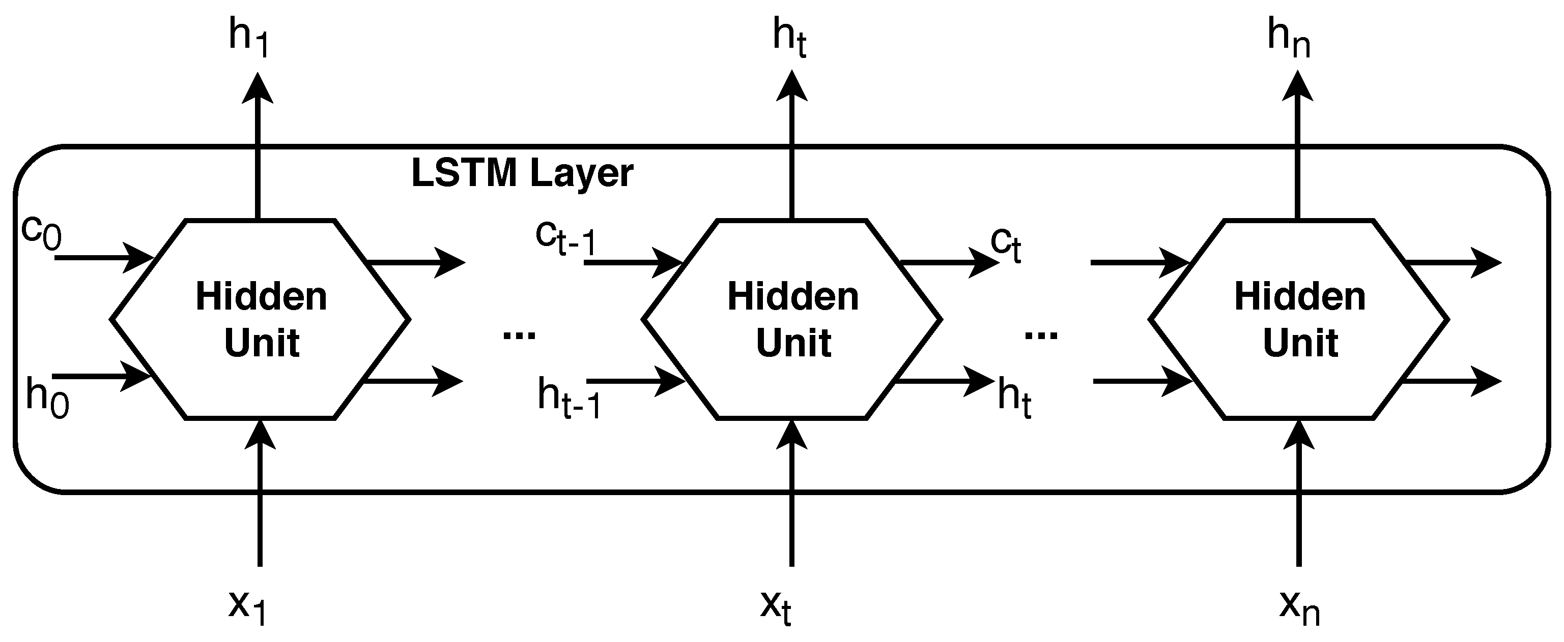
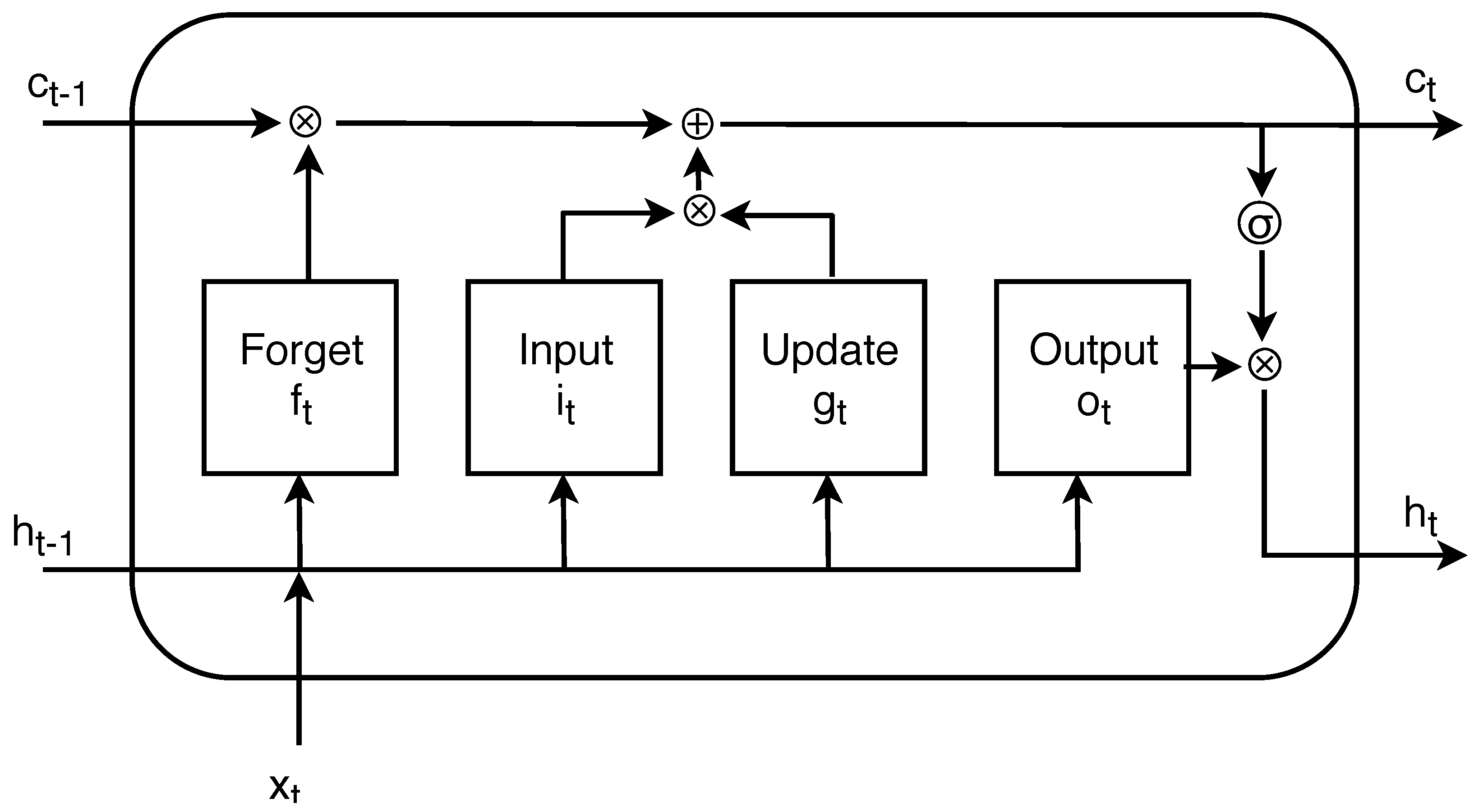
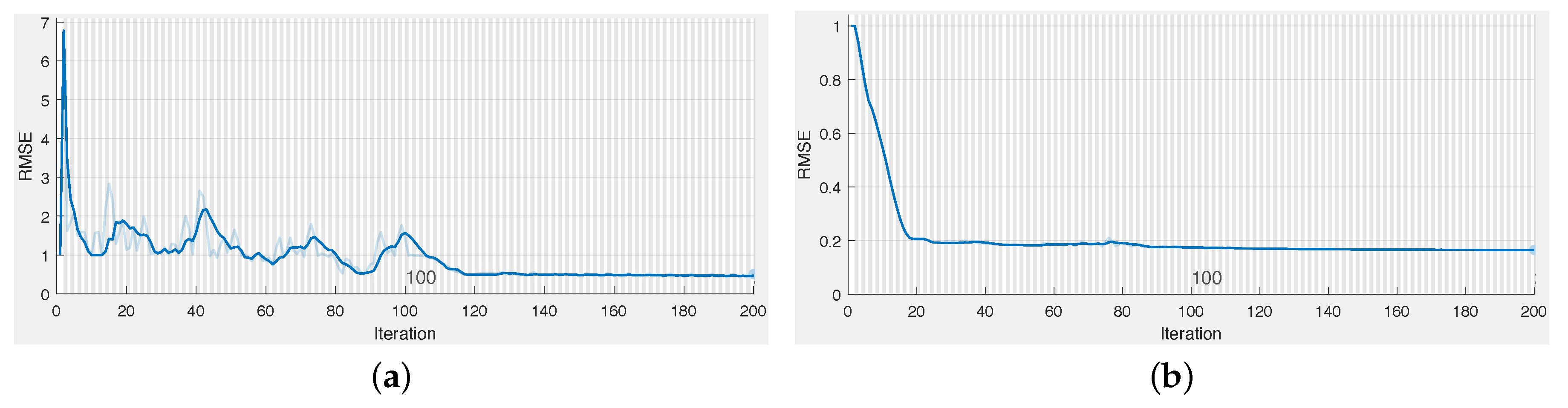
3.1. RNN Implementation with LSTM
- input gate —level of cell state update;
- layer update —add information to cell state;
- forget gate —remove information from cell state;
- output gate —effect of cell state on output.
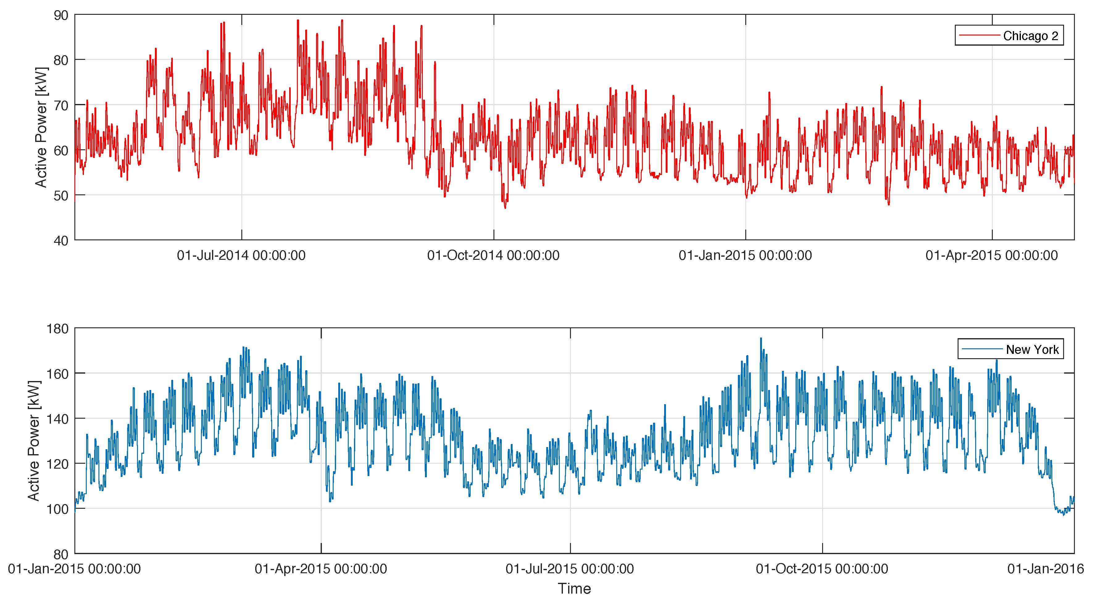
3.2. Benchmarking Datasets
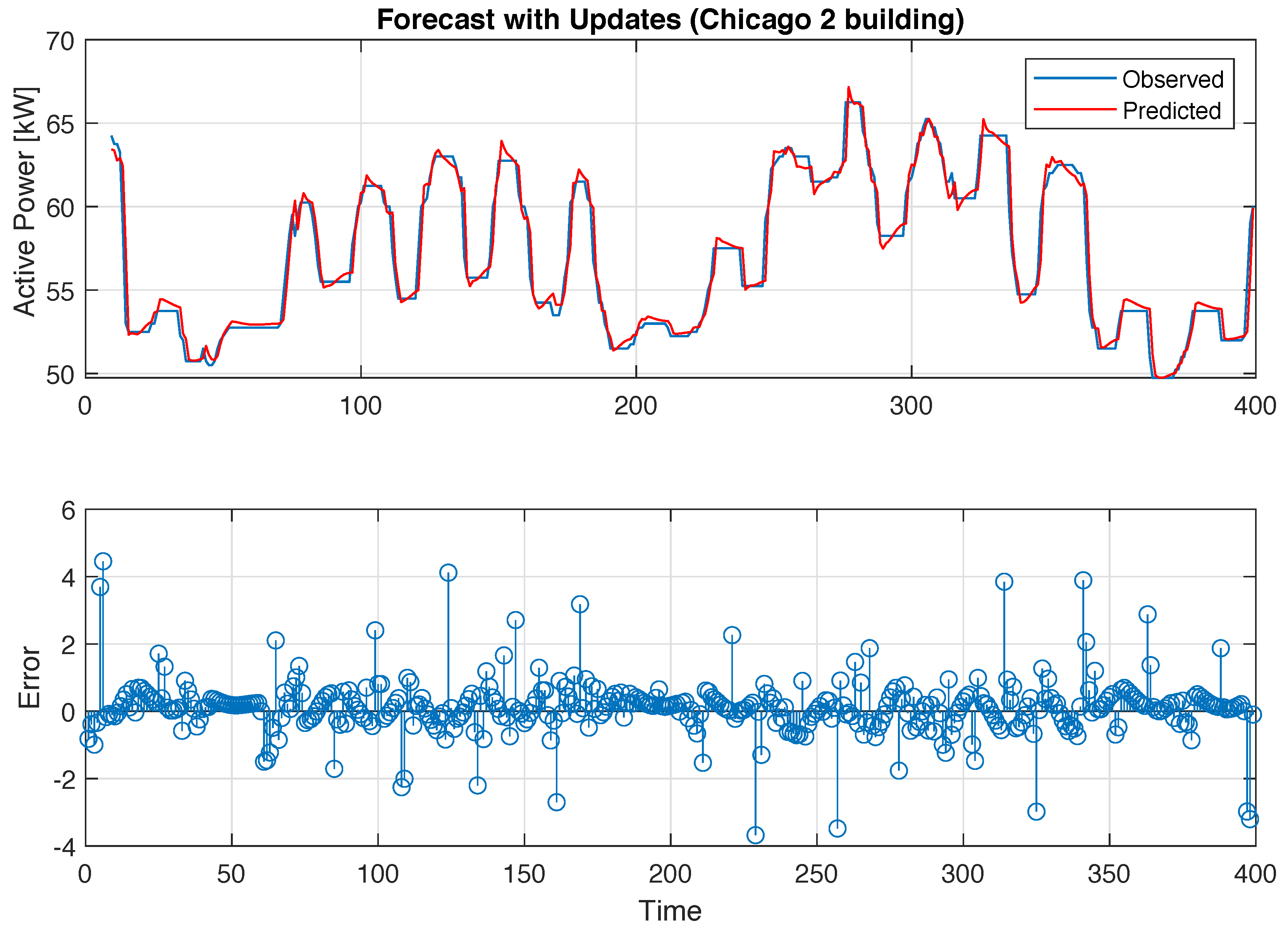
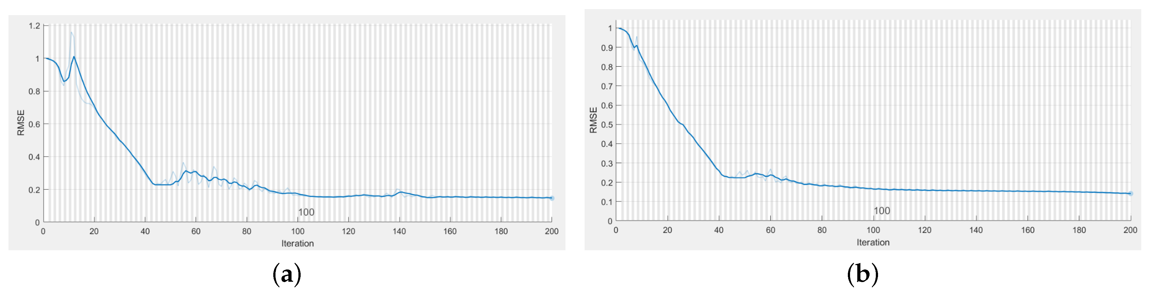
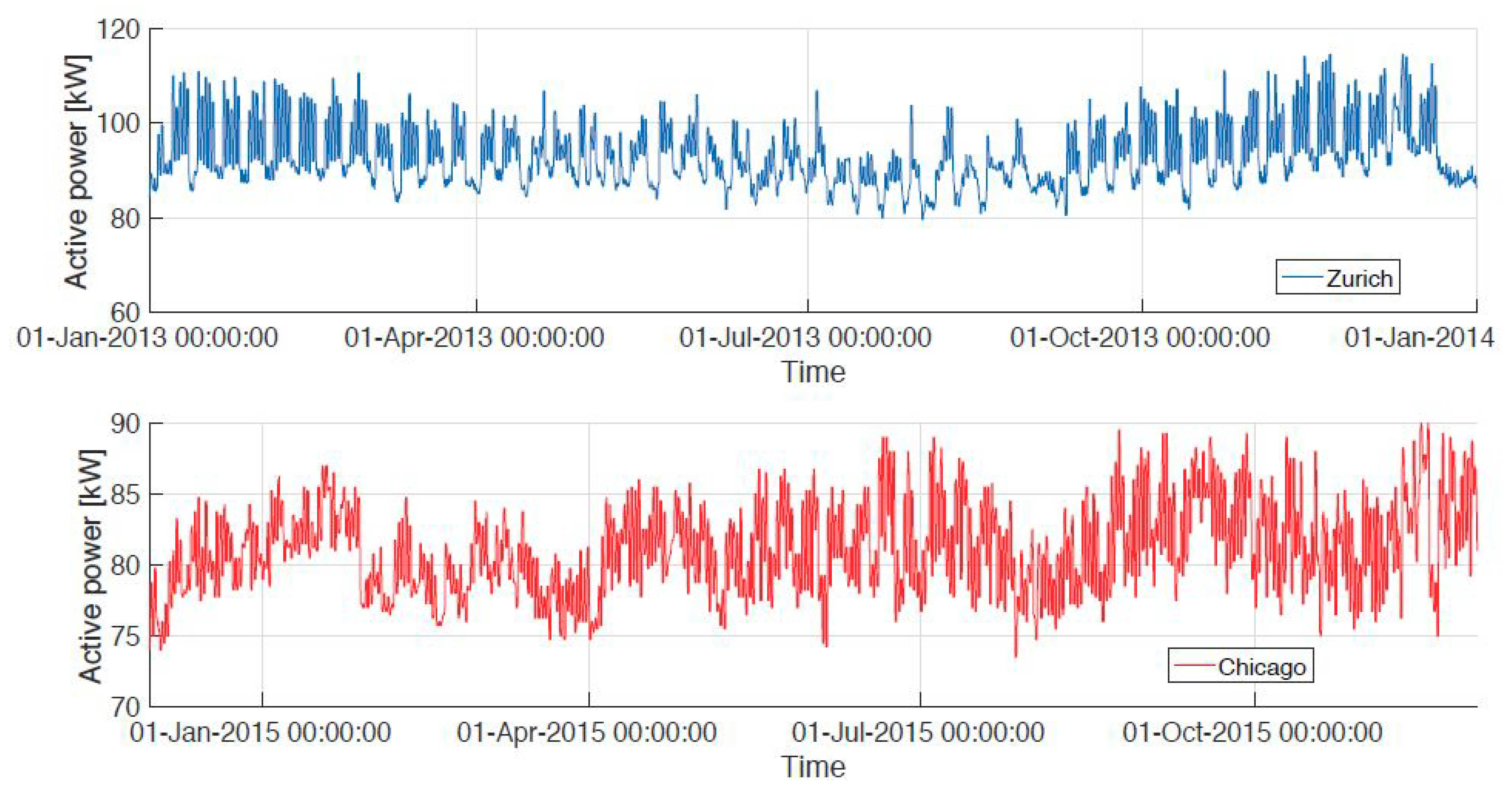
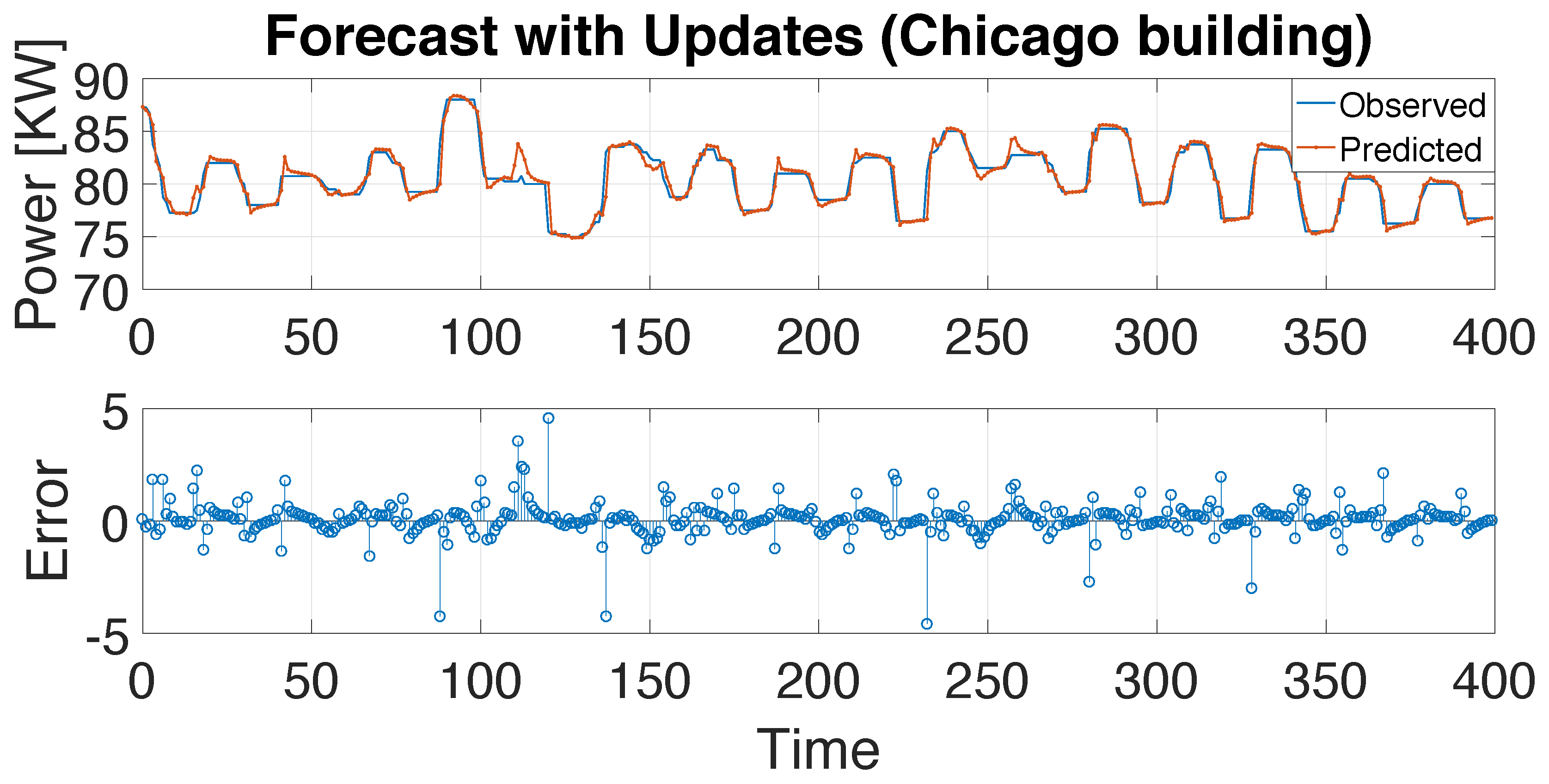
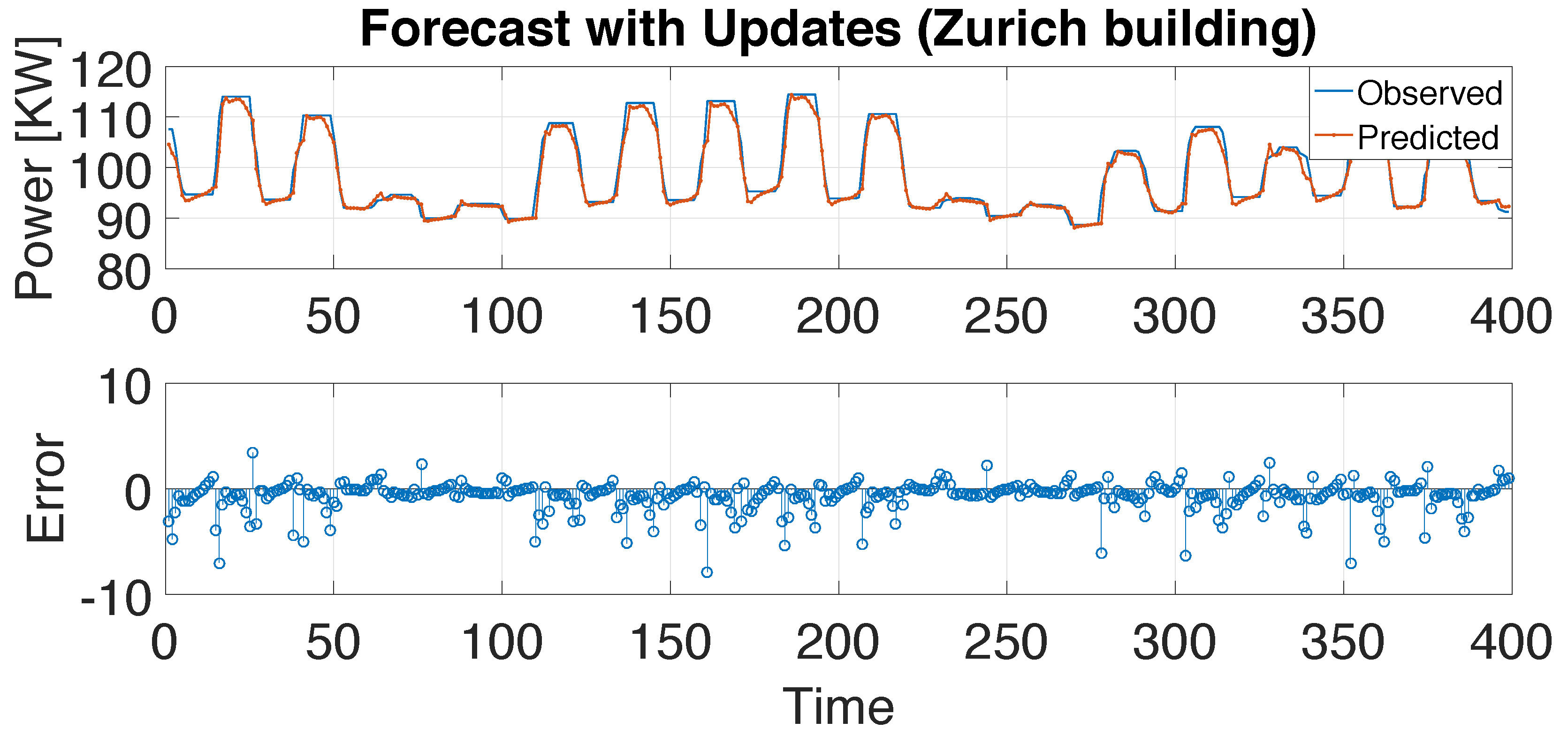
4. Experiment Evaluation for Building-Energy Time-Series Forecasting
5. Conclusions
Author Contributions
Funding
Conflicts of Interest
Abbreviations
| ADAM | Adaptive Moment Estimation |
| ARIMA | Autoregressive Integrated Moving Average |
| BPTT | Back-Propagation Through Time |
| CV (RMSE) | Coefficient of Variation of RMSE |
| LSTM | Long Short-Term Memory |
| DL | Deep Learning |
| GRU | Gated Recurrent Unit |
| MAPE | Mean Absolute Percentage Error |
| MSE | Mean Squared Error |
| RMSE | Root Mean Squared Error |
| RNN | Recurrent Neural Network |
| RTRL | Real-Time Recurrent Learning |
References
- Berardi, U. Building Energy Consumption in US, EU, and BRIC Countries. Procedia Eng. 2015, 118, 128–136. [Google Scholar] [CrossRef] [Green Version]
- Djenouri, D.; Laidi, R.; Djenouri, Y.; Balasingham, I. Machine Learning for Smart Building Applications: Review and Taxonomy. ACM Comput. Surv. 2019, 52, 24:1–24:36. [Google Scholar] [CrossRef]
- Nichiforov, C.; Stamatescu, G.; Stamatescu, I.; Calofir, V.; Fagarasan, I.; Iliescu, S.S. Deep Learning Techniques for Load Forecasting in Large Commercial Buildings. In Proceedings of the 2018 22nd International Conference on System Theory, Control and Computing (ICSTCC), Sinaia, Romania, 10–12 October 2018; pp. 492–497. [Google Scholar] [CrossRef]
- Fayaz, M.; Shah, H.; Aseere, A.M.; Mashwani, W.K.; Shah, A.S. A Framework for Prediction of Household Energy Consumption Using Feed Forward Back Propagation Neural Network. Technologies 2019, 7, 30. [Google Scholar] [CrossRef]
- Wang, X.; Zhang, M.; Ren, F. Learning Customer Behaviors for Effective Load Forecasting. IEEE Trans. Knowl. Data Eng. 2019, 31, 938–951. [Google Scholar] [CrossRef]
- Aminikhanghahi, S.; Wang, T.; Cook, D.J. Real-Time Change Point Detection with Application to Smart Home Time Series Data. IEEE Trans. Knowl. Data Eng. 2019, 31, 1010–1023. [Google Scholar] [CrossRef]
- Jin, M.; Bekiaris-Liberis, N.; Weekly, K.; Spanos, C.J.; Bayen, A.M. Occupancy Detection via Environmental Sensing. IEEE Trans. Autom. Sci. Eng. 2018, 15, 443–455. [Google Scholar] [CrossRef]
- Rahman, A.; Srikumar, V.; Smith, A.D. Predicting electricity consumption for commercial and residential buildings using deep recurrent neural networks. Appl. Energy 2018, 212, 372–385. [Google Scholar] [CrossRef]
- Fan, C.; Sun, Y.; Zhao, Y.; Song, M.; Wang, J. Deep learning-based feature engineering methods for improved building energy prediction. Appl. Energy 2019, 240, 35–45. [Google Scholar] [CrossRef]
- Zhong, H.; Wang, J.; Jia, H.; Mu, Y.; Lv, S. Vector field-based support vector regression for building energy consumption prediction. Appl. Energy 2019, 242, 403–414. [Google Scholar] [CrossRef]
- Harish, V.; Kumar, A. Reduced order modeling and parameter identification of a building energy system model through an optimization routine. Appl. Energy 2016, 162, 1010–1023. [Google Scholar] [CrossRef]
- Capizzi, G.; Sciuto, G.L.; Cammarata, G.; Cammarata, M. Thermal transients simulations of a building by a dynamic model based on thermal-electrical analogy: Evaluation and implementation issue. Appl. Energy 2017, 199, 323–334. [Google Scholar] [CrossRef]
- Nichiforov, C.; Stamatescu, I.; Făgărăşan, I.; Stamatescu, G. Energy consumption forecasting using ARIMA and neural network models. In Proceedings of the 2017 5th International Symposium on Electrical and Electronics Engineering (ISEEE), Galaţi, Romania, 20–22 October 2017; pp. 1–4. [Google Scholar] [CrossRef]
- Nichiforov, C.; Stamatescu, G.; Stamatescu, I.; Fagarasan, I.; Iliescu, S.S. Intelligent Load Forecasting for Building Energy Management. In Proceedings of the 2018 14th IEEE International Conference on Control and Automation (ICCA), Anchorage, AK, USA, 12–15 June 2018. [Google Scholar]
- Stamatescu, I.; Arghira, N.; Fagarasan, I.; Stamatescu, G.; Iliescu, S.S.; Calofir, V. Decision Support System for a Low Voltage Renewable Energy System. Energies 2017, 10, 118. [Google Scholar] [CrossRef]
- Werbos, P.J. Backpropagation through time: What it does and how to do it. Proc. IEEE 1990, 78, 1550–1560. [Google Scholar] [CrossRef]
- Williams, R.J.; Zipser, D. Gradient-based learning algorithms for recurrent networks and their computational complexity. In Developments in Connectionist Theory. Backpropagation: Theory, Architectures, and Applications; Erlbaum Associates Inc.: Hillsdale, NJ, USA, 1995; pp. 433–486. [Google Scholar]
- Hochreiter, S.; Schmidhuber, J. Long Short-Term Memory. Neural Comput. 1997, 9, 1735–1780. [Google Scholar] [CrossRef] [PubMed]
- Marino, D.L.; Amarasinghe, K.; Manic, M. Building Energy Load Forecasting using Deep Neural Networks. arXiv 2016, arXiv:1610.09460. [Google Scholar]
- Srivastava, S.; Lessmann, S. A comparative study of LSTM neural networks in forecasting day-ahead global horizontal irradiance with satellite data. Sol. Energy 2018, 162, 232–247. [Google Scholar] [CrossRef]
- Chung, J.; Gülçehre, Ç.; Cho, K.; Bengio, Y. Empirical Evaluation of Gated Recurrent Neural Networks on Sequence Modeling. arXiv 2014, arXiv:1412.3555. [Google Scholar]
- Ugurlu, U.; Oksuz, I.; Tas, O. Electricity Price Forecasting Using Recurrent Neural Networks. Energies 2018, 11, 1255. [Google Scholar] [CrossRef]
- Miller, C.; Meggers, F. The Building Data Genome Project: An open, public data set from non-residential building electrical meters. Energy Procedia 2017, 122, 439–444. [Google Scholar] [CrossRef]
- Broesch, J.D. Chapter 7—Applications of DSP. In Digital Signal Processing; Broesch, J.D., Ed.; Instant Access, Newnes: Burlington, NJ, USA, 2009; pp. 125–134. [Google Scholar] [CrossRef]
- Kingma, D.P.; Ba, J. Adam: A Method for Stochastic Optimization. arXiv 2014, arXiv:1412.6980. [Google Scholar]
- Stamatescu, G.; Stamatescu, I.; Arghira, N.; Făgărăsan, I.; Iliescu, S.S. Embedded networked monitoring and control for renewable energy storage systems. In Proceedings of the 2014 International Conference on Development and Application Systems (DAS), Suceava, Romania, 15–17 May 2014; pp. 1–6. [Google Scholar] [CrossRef]


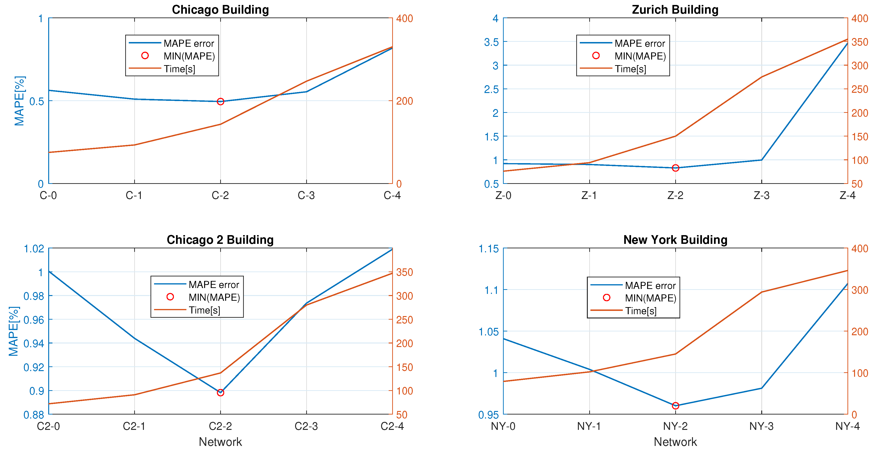
| C-0 | C-1 | C-2 | C-3 | C-4 | |
|---|---|---|---|---|---|
| Time(s) | 75 | 93 | 143 | 247 | 330 |
| MSE | 0.6295 | 0.6132 | 0.5553 | 0.7486 | 0.9555 |
| RMSE | 0.7934 | 0.7831 | 0.7452 | 0.8652 | 0.9775 |
| CV(RMSE)(%) | 0.98 | 0.97 | 0.92 | 1.07 | 1.2 |
| MAPE(%) | 0.5623 | 0.5091 | 0.4945 | 0.5535 | 0.8177 |
| Z-0 | Z-1 | Z-2 | Z-3 | Z-4 | |
|---|---|---|---|---|---|
| Time(s) | 76 | 94 | 150 | 275 | 355 |
| MSE | 2.3846 | 2.1732 | 2.0506 | 2.2506 | 2.034 |
| RMSE | 1.5442 | 1.4742 | 1.432 | 1.5002 | 1.5107 |
| CV(RMSE)(%) | 1.66 | 1.59 | 1.58 | 1.61 | 1.63 |
| MAPE(%) | 0.9197 | 0.9008 | 0.828 | 0.9958 | 3.4684 |
| C2-0 | C2-1 | C2-2 | C2-3 | C2-4 | |
|---|---|---|---|---|---|
| Time(s) | 72 | 91 | 137 | 280 | 347 |
| MSE | 0.8013 | 0.7801 | 0.7163 | 0.7626 | 0.8413 |
| RMSE | 0.8952 | 0.8832 | 0.8464 | 0.8733 | 0.9172 |
| CV(RMSE)(%) | 1.63 | 1.6 | 1.53 | 1.57 | 1.65 |
| MAPE(%) | 1.0005 | 0.9439 | 0.8982 | 0.9736 | 1.019 |
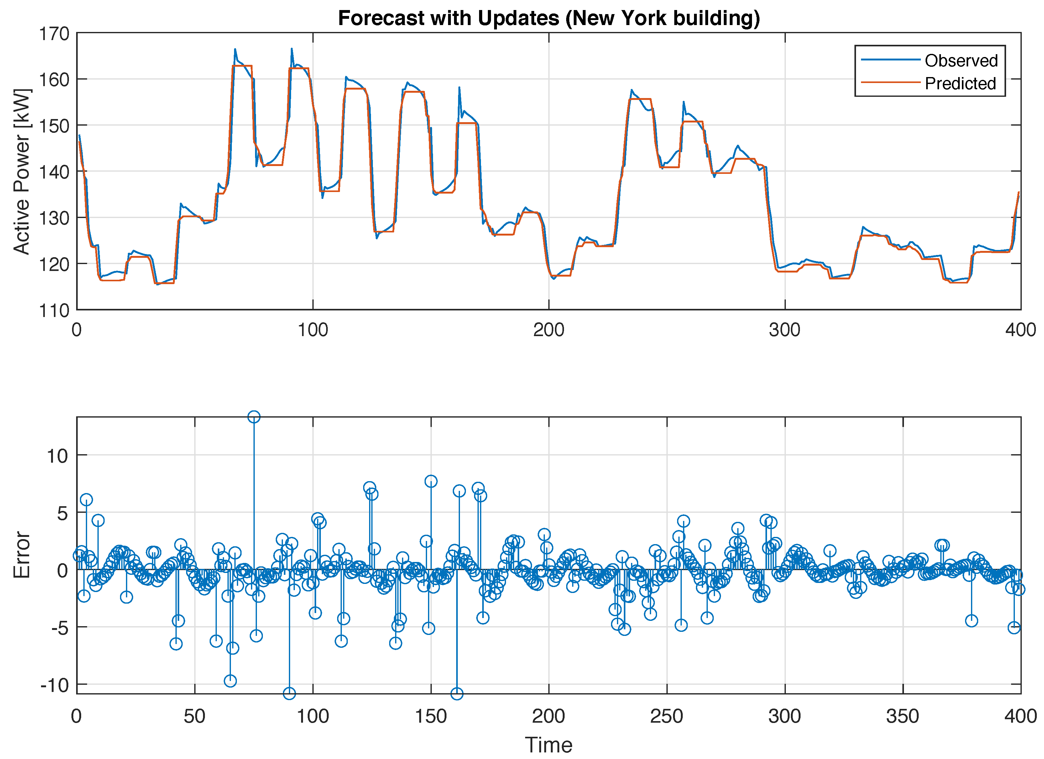
| NY-0 | NY-1 | NY-2 | NY-3 | NY-4 | |
|---|---|---|---|---|---|
| Time(s) | 79 | 102 | 145 | 294 | 346 |
| MSE | 5.4433 | 5.4012 | 4.7778 | 5.1203 | 5.5522 |
| RMSE | 2.3309 | 2.3241 | 2.1858 | 2.2628 | 2.3563 |
| CV(RMSE)(%) | 1.75 | 1.73 | 1.7 | 1.72 | 1.78 |
| MAPE(%) | 1.0409 | 1.004 | 0.9602 | 0.9813 | 1.1073 |
| Min | Max | s | k | |||
|---|---|---|---|---|---|---|
| CV (RMSE) | 0.92 | 1.78 | 1.4935 | 0.2873 | −1.0846 | 2.5502 |
| MAPE | 0.4945 | 3.4684 | 0.9989 | 0.6108 | 3.4661 | 14.8790 |
© 2019 by the authors. Licensee MDPI, Basel, Switzerland. This article is an open access article distributed under the terms and conditions of the Creative Commons Attribution (CC BY) license (http://creativecommons.org/licenses/by/4.0/).
Share and Cite
Nichiforov, C.; Stamatescu, G.; Stamatescu, I.; Făgărăşan, I. Evaluation of Sequence-Learning Models for Large-Commercial-Building Load Forecasting. Information 2019, 10, 189. https://doi.org/10.3390/info10060189
Nichiforov C, Stamatescu G, Stamatescu I, Făgărăşan I. Evaluation of Sequence-Learning Models for Large-Commercial-Building Load Forecasting. Information. 2019; 10(6):189. https://doi.org/10.3390/info10060189
Chicago/Turabian StyleNichiforov, Cristina, Grigore Stamatescu, Iulia Stamatescu, and Ioana Făgărăşan. 2019. "Evaluation of Sequence-Learning Models for Large-Commercial-Building Load Forecasting" Information 10, no. 6: 189. https://doi.org/10.3390/info10060189
APA StyleNichiforov, C., Stamatescu, G., Stamatescu, I., & Făgărăşan, I. (2019). Evaluation of Sequence-Learning Models for Large-Commercial-Building Load Forecasting. Information, 10(6), 189. https://doi.org/10.3390/info10060189