Information Matrix-Based Adaptive Sampling in Hull Form Optimisation

Abstract

Hull form optimisation involves challenges such as large design spaces, numerous design variables, and high nonlinearity. Therefore, optimisation that only use global approximate models alone cannot yield desirable results. An information matrix-based method is proposed for dynamically embedded local approximate models (IM-DEAM) in this paper, which uses the Gaussian-function information matrix to extract one or more subspaces for additional sampling and a Latin hypercube design (LHD) for adaptive sampling. In addition, to prevent overfitting by global approximate models in some spaces because of the uneven distribution of the samples, local approximate models are embedded in the subspaces identified for additional sampling to enable accurate description of subspaces. The effectiveness and robustness of the method are validated and analysed by applying the proposed method to optimise mathematical functions and the hull form of the DTMB 5415. The results demonstrate that the proposed method is effective for improving the accuracies and can produce reliable optimisation results.

1. Introduction

High-accuracy approximate models are usually used as surrogates of complex, time-consuming computational fluid dynamics (CFD) and finite element method (FEM) [1,2,3,4,5]. Approximate modelling has become an important branch of multidisciplinary design optimisation being researched [6].

Building approximate models with acceptable prediction accuracies using few samples is a challenge. For example, Prebeg et al. [7] and Žanić et al. [8] tested the usefulness of different approximation models for the modelling of structural responses using few samples. Generally, there are two types of methods for approximate modelling [9,10]: one-shot sampling-based method [11] and dynamic sampling-based methods [12,13]. One-shot sampling determines the number of samples for the experimental design, that is, sampling only once. However, for engineering optimization problems without prior knowledge, it is difficult to determine the appropriate or optimal sampling capacity. In view of the limitations and deficiencies of the one-shot sampling strategy, a dynamic sampling (or adaptive sampling) strategy is proposed to improve the accuracy and development of the approximate model in the entire design space, which allows the selection of sample points through the approximate model or the data it learns. For engineering optimisation problems without a priori knowledge, one-shot sampling may result in an undersampling of the objective function or in an excessive number of training points [14]. In contrast, dynamic sampling, which does not have the limitations and deficiencies of one-shot sampling, involves sampling of additional points in regions with significant errors [15,16,17] or potential optimum regions [18,19,20,21,22,23,24], thereby enabling the construction of more accurate approximate models with less sample points.

In recent years, several dynamic sampling-based methods have been proposed for approximate modelling. Jiang et al. [15] and Chang et al. [24] used leave-one-out (LOO) method-based sequential sampling to improve the model prediction accuracy in the output space while considering the filling characteristics of the input space. Beck and Guillas [16] proposed a mutual information for computer experiment (MICE)-based adaptive sequential sampling algorithm that adaptively selected design values at which to run the computer simulator to maximise the expected information gain over the input space. Xu et al. [17] used a Voronoi method for space partition and cross validation for adaptively sampling additional points in the cell with the largest error. Zhu and Du [18] used a learning function for selecting new training points based on information obtained by Kriging models and Monte Carlo simulations (MCS). Žanić and Čudina [25] pointed out that inadequate information about configuration of feasible designs subspace is overcome by adaptive Monte Carlo (AMC) method generation of design points in feasible region. Ye and Pan [19] integrated three types of representative global approximate models with optimised weight factors and used a fuzzy clustering technique to reduce the design space, thereby identifying the subspaces of interest and obtaining promising sample points in sparse subspaces to prevent premature convergence to local optima. Yu et al. [22] proposed an adaptive surrogate model (ASM) selection technique-based dynamic surrogate-assisted evolutionary algorithm (SAEA), in which a combination of promising elite models was adaptively selected from the model strategy pool based on the minimum root of mean square error (RMSE), thereby providing reliable approximate model combinations for the optimisation process. Li et al. [21] proposed a global optimisation method that integrated a fuzzy-clustering, adaptive-infilling algorithm into the Kriging model-based optimisation. The optimisation method partitioned the design space into several subspaces and selected new infilling samples in the subspaces by maximising the expected improvement of the objective function and minimising surrogate prediction (MSP), and finally merged the subspaces to refine and reduce the design space. Yu et al. [20] proposed a generation-based optimal restart strategy for surrogate-assisted social learning particle swarm optimisation (GORS-SSLPSO), in which particles were restarted by selecting optimal samples in a radial-basis function (RBF) model using the social learning particle swarm algorithm and the accuracy of the RBF model was improved by selecting the promising individuals with the optimal RBF estimates for exact evaluation. Cai et al. [23] developed an algorithm that efficiently used the optimum information obtained from global approximate models and approximate models of local optimum regions. The approximate model-assisted particle swarm algorithm was capable of relatively accurate and efficient search.

However, in some cases, the dynamic sampling-based global approximate models are prone to overfitting, which leads to the missing of global optima and the reduced reliability of optimisation results. Therefore, in this paper, a method was proposed for the information matrix-based dynamic embedding of approximate methods (IM-DEAM). Local approximate models were embedded (EAM) in subspaces with additional sample points to improve the local-region prediction accuracy and assist global approximate models in optimisation.

This paper is structured as follows. Firstly, the general framework of dynamic approximation model construction based on adaptive sampling is briefly introduced. Section 2 describes the adaptive sampling method based on information matrix and the local embedded approximation model technique. Section 3 validates the effectiveness and robustness of the method by applying it to mathematical functions. Section 4 applies the method to hull form optimisation. Finally, Section 5 summarises the conclusions.

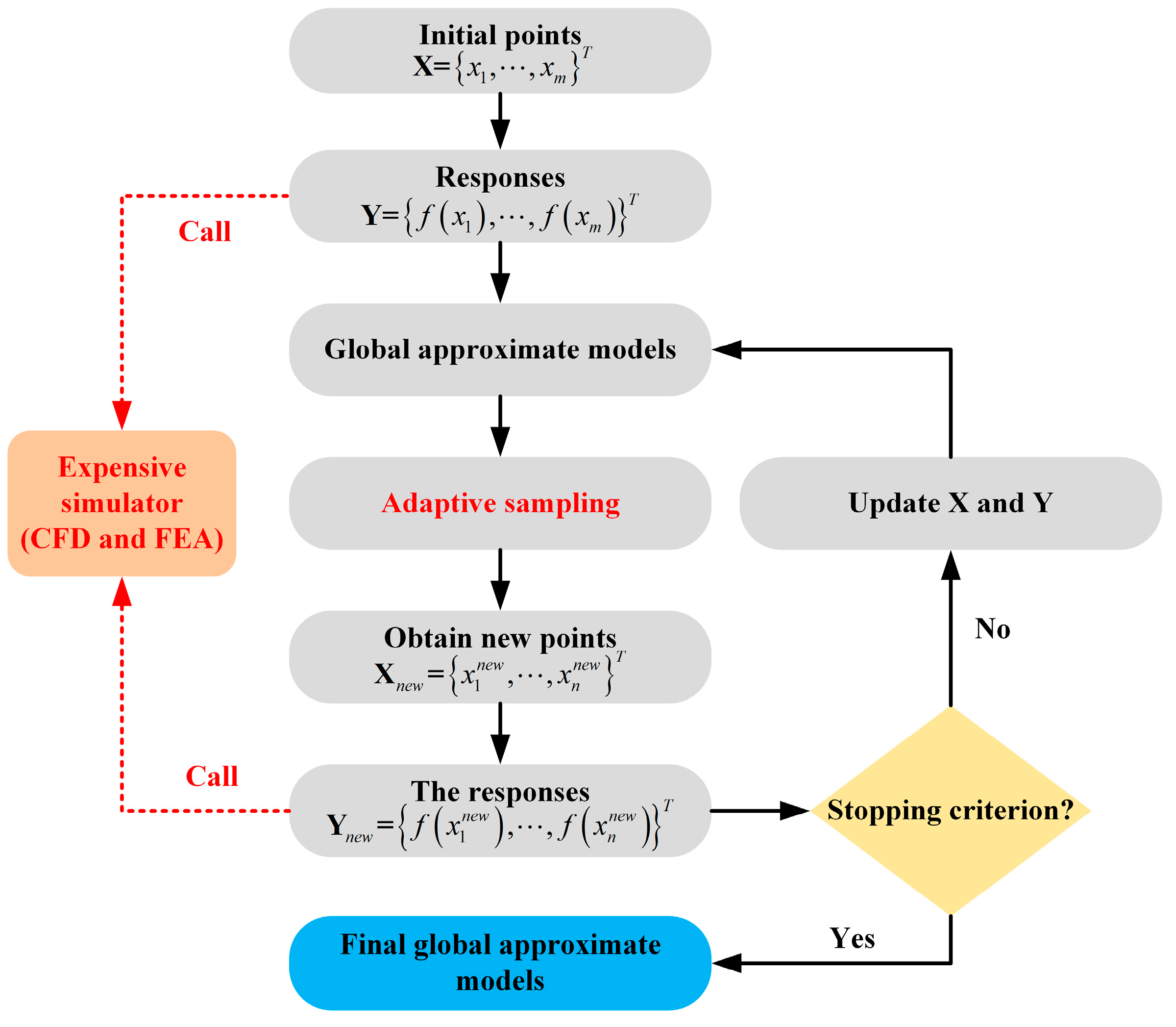
Dynamical Construction for Global Approximate Model

Dynamical construction of the approximate models requires sampling design points that are analysed via the realistic engineering models, then the approximate models are built. The sampling points are typically generated by adaptive sampling methods, which is designed for scenarios where the output responses of sample points are very expensive to obtain. In the field of machine learning, adaptive sampling, known as active learning, is described as “… the key hypothesis is that if the learning algorithm is allowed to choose the data from which it learns-to be “curious”, if you will-it will perform better with less training.” [13]. For global metamodeling, adaptive sampling seeks the potential informative points for building accurate global approximate models with less computing cost. Therefore, the adaptive sampling method has gained popularity for its advantages of flexibility and adaptability over other methods.

Figure 1 depicts a general adaptive sampling process for global dynamical approximate models. The process begins with a small number of initial sample points X = {x₁, x₂, …, x_m}^T and Y = {f(x₁), f (x₂), …, f (x_m)}^T by calling the numerical simulation (CFD or FEM), which are used to construct the initial approximation model. Based on an adaptive sampling criterion, it then solves an auxiliary optimization problem to iteratively add new sample points X_new and Y_new, which are used to update the training sample set and the approximate model until a stopping criterion is met.

Unlike current global dynamical approximate models, a dynamic embedded approximate model based on information matrix is proposed to enhance the approximate model reliability in this paper. More details about the proposed approach will be introduced in Section 2. The local approximate model reconstruction is embedded in the framework of the general global dynamical approximate model in Figure 1 (see Section 2.2).

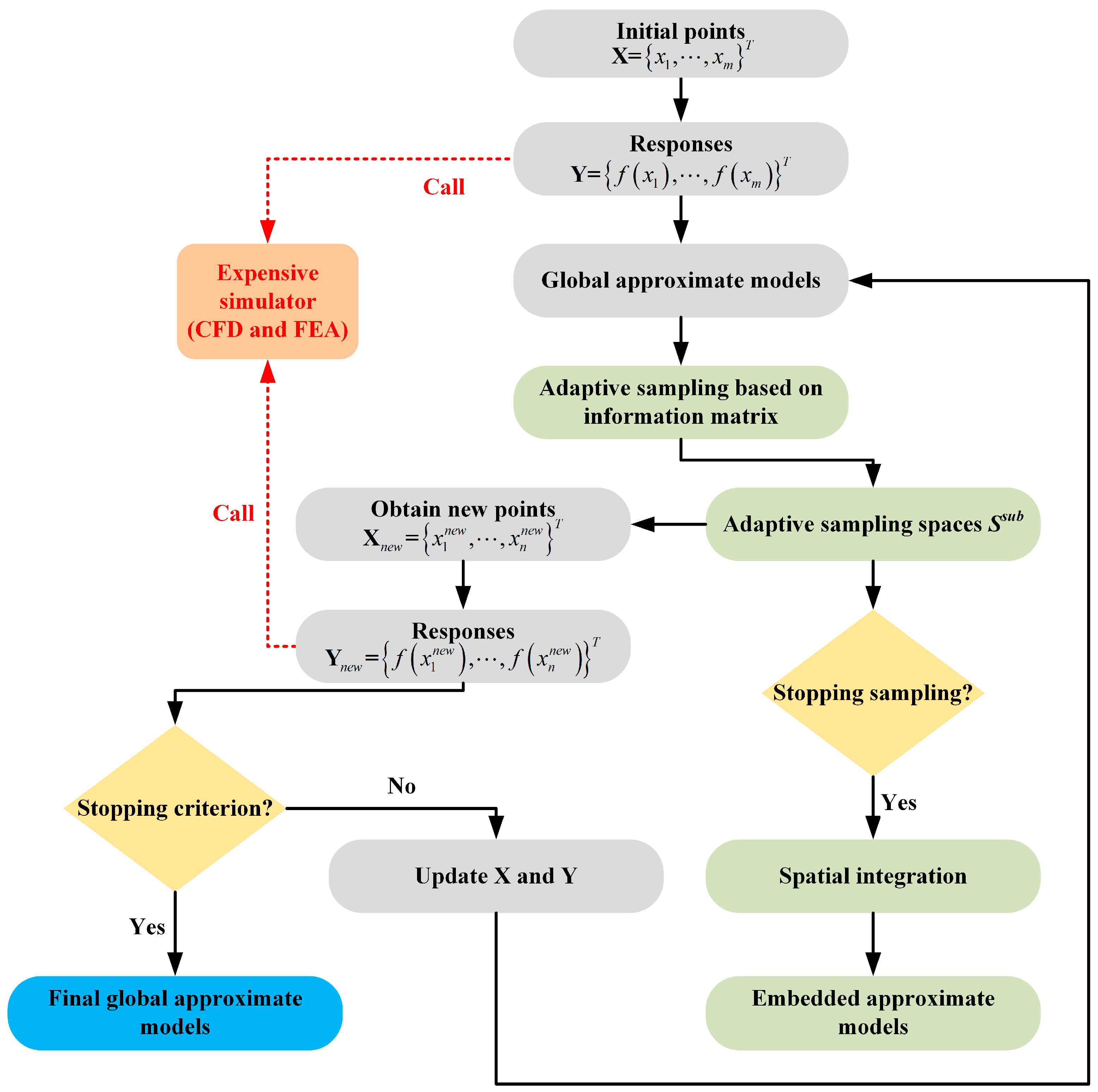
2. Materials and Methods

Determining the subspaces for additional sampling is a critical step in adaptive sampling. This section describes the construction of a sample information matrix and the use of the coefficients of correlation between the samples in the information matrix for determining the subspaces for additional sampling. In addition, to eliminate the potential overfitting by global approximate models during sampling, local approximate models are constructed in the identified subspaces for accurately describing the local regions of the target space. Finally, based on these two methods, the information matrix-based dynamically embedded approximate models (IM-DEAM) is proposed.

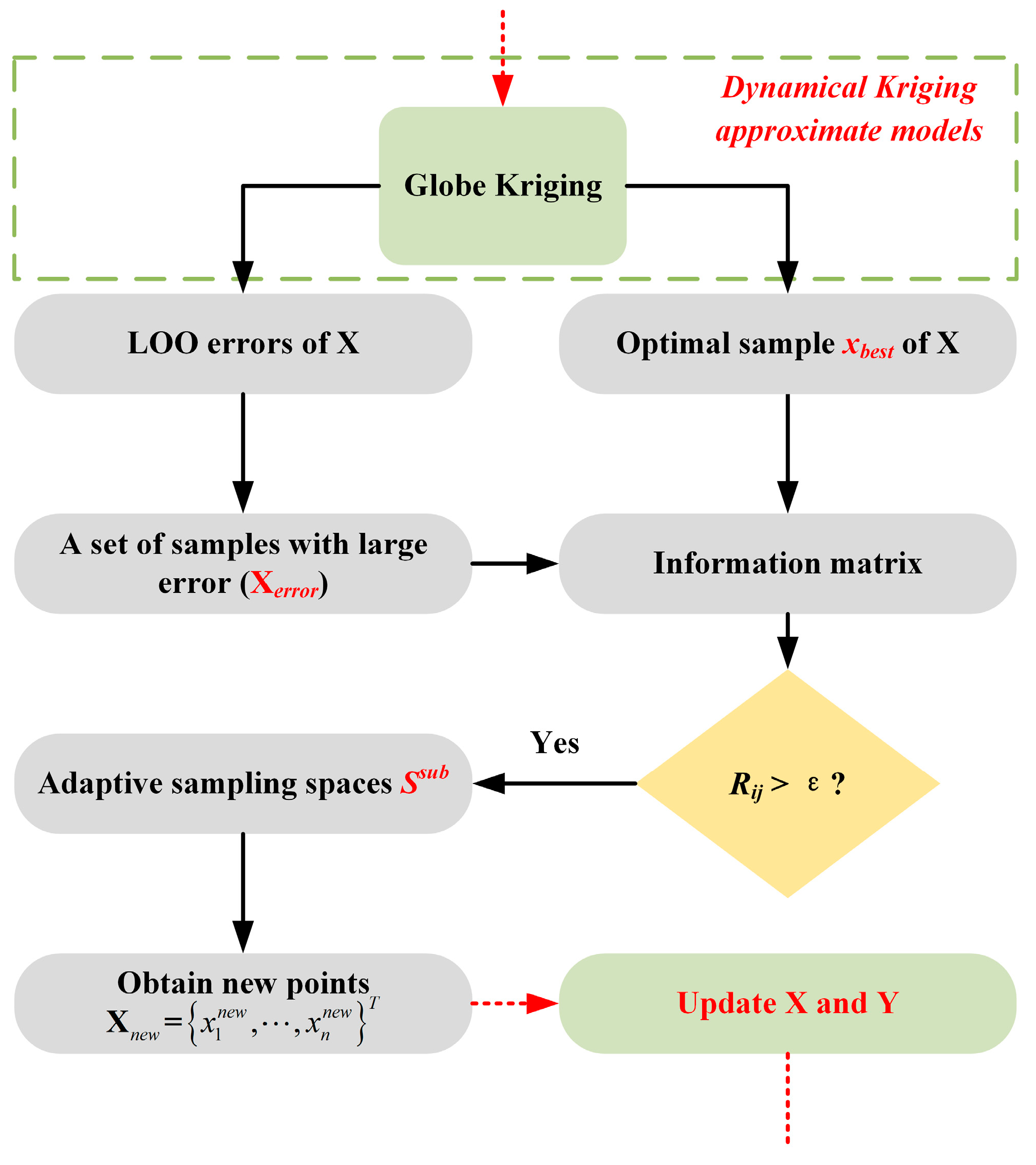
2.1. Adaptive Sampling with the Information Matrix

For the sample set X = {x₁, x₂, …, x_m}^T, this study utilizes the Kriging model to construct an approximate model. Kriging combines a global model and a local component:

$$y\left(x\right)=F\left(x\right)\beta +Z\left(x\right)$$

(1)

where, F(x) is a polynomial function of order 0, 1, or 2 of x, β is a coefficient vector (when F(x) is a unit column vector, β is a constant), and Z(x) follows a random distribution of mean 0 and variance σ².

F(x) is a unit column vector, then Equation (1) is:

$$y\left(x\right)=\beta +r\left(x\right){\mathbf{R}}^{-1}\left(\mathbf{Y}-\mathbf{1}\beta \right)$$

(2)

where, Y = {y₁, y₂, …, y_m}^T is the m-dimensional column vector composed of sample fitness, R is the correlation matrix.

For the specific derivation of Kriging, please refer to DACE [26]. This section mainly introduces the correlation function and the correlation matrix R.

Based on the stationarity assumption, in the absence of prior knowledge, the covariance of two points is only a function of their distance and does not depend on their position in the design space. It is, in some sense, a non-informational and non-discriminatory assumption [27]. The information matrix R (i.e., correlation function matrix) of samples consists of the coefficients of correlation between the samples. It is used for characterising the correlations between them, that is, the degrees of mutual influence between the samples. The correlation function is a function with respect to distance and is used to calculate the coefficients of correlation between samples. The general form of the correlation function is as follows:

$$R\left(\theta ,x^i,x^j\right)={\displaystyle \prod _{d=1}^D{R}_d\left({\theta }_d,x_d^i-x_d^j\right)}$$

(3)

where xⁱ is the ith sample in the set of initial samples, θ_d is the hyperparameter of the correlation function in the dth dimension, and D is the number of variables.

For convenience, R(θ, xⁱ, x^j) is denoted as R_ij hereafter. At present, the coefficients of correlation between samples are usually calculated using the following exponential function:

$$R_{ij}=\exp \left(-{\displaystyle \sum _{d=1}^D{\theta }_d{\left|x_d^i-x_d^j\right|}^p}\right),0<p\le 2$$

(4)

Then the information matrix R is obtained:

$$\mathbf{R}=\left[\begin{array}{cccc}{R}_{11}& R_{12}& \cdots & R_{1m}\\ R_{21}& \ddots & \cdots & R_{2m}\\ ⋮& ⋮& \ddots & ⋮\\ R_{m1}& R_{m2}& \cdots & R_{mm}\end{array}\right]$$

(5)

Equation (4) contains two unknowns: θ_d and p. The value of θ_d indicates the influenced extension of the variable. The value of p affects the smoothness of the function. In order to clearly show the influence of the two parameters on the correlation function, the one-dimensional (1D) Gaussian exponential function indicator function is shown in Figure 2.

For all curves in Figure 2a,b, the value of R_ij decreases as the distance increases, that is, the correlation between samples weakens as the distance increases. Two samples with a distance larger than a certain value are considered not correlated. In addition, a larger value of θ leads to a more rapid decrease in the coefficient of correlation, that is, a smaller threshold value of the distance for the absence of correlation. Figure 2a,b indicates that the Gaussian correlation function (p = 2) has parabolic curves near the origin. This implies that, for continuously differentiable problems, the Gaussian correlation function leads to a higher level of smoothness. Therefore, in this study, the Gaussian correlation function is used to calculate sample information matrices and construct the globe Kriging model.

It is found that the LOO cross-validation (CV) errors [28] are able to estimate the local prediction errors to some extent. A small LOO-CV error implies that the model accuracy is insensitive to the loss of x_i, that is, the approximate model has been well fitted around x_i; while on the contrary, a large LOO-CV error indicates that the region around x_i does not contain enough points such that the model accuracy is significantly affected by the loss of x_i.

Figure 3 depicts the flowchart for adaptive sampling with the information matrix. For a globe Kriging model, it can provide the correlation coefficient R_ij between the x_i and x_j. Based on the globe Kriging model, the LOO can also provide the errors of each sample in the sample set X. Then based on the LOO errors, the samples with a large error are obtained, i.e., X_error and the optimal sample x_best ∈ X is obtained. The remaining samples X_Rij > ε meeting the judgment conditions R_ij > ε (ε = 0.01) can be obtained through the information matrix R for x_best and every sample in X_error. Finally, the spaces S^sub centred on sample x_i ∈ {X_error, x_best} containing the sample set X_Rij > ε is the sampling space in which new sample points $x_i^{\mathit{new}}$ ∈ X_new are obtained by DOE.

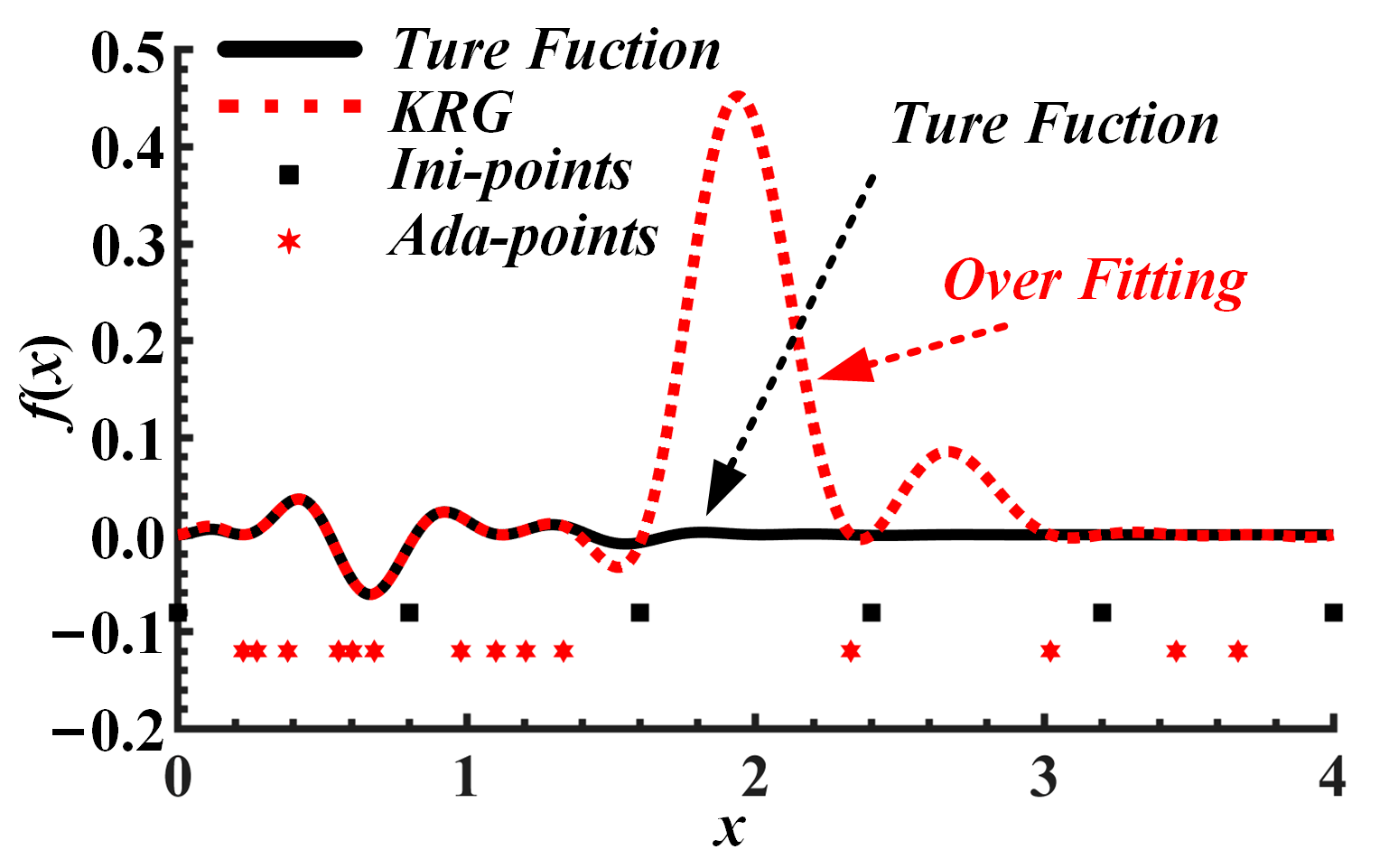
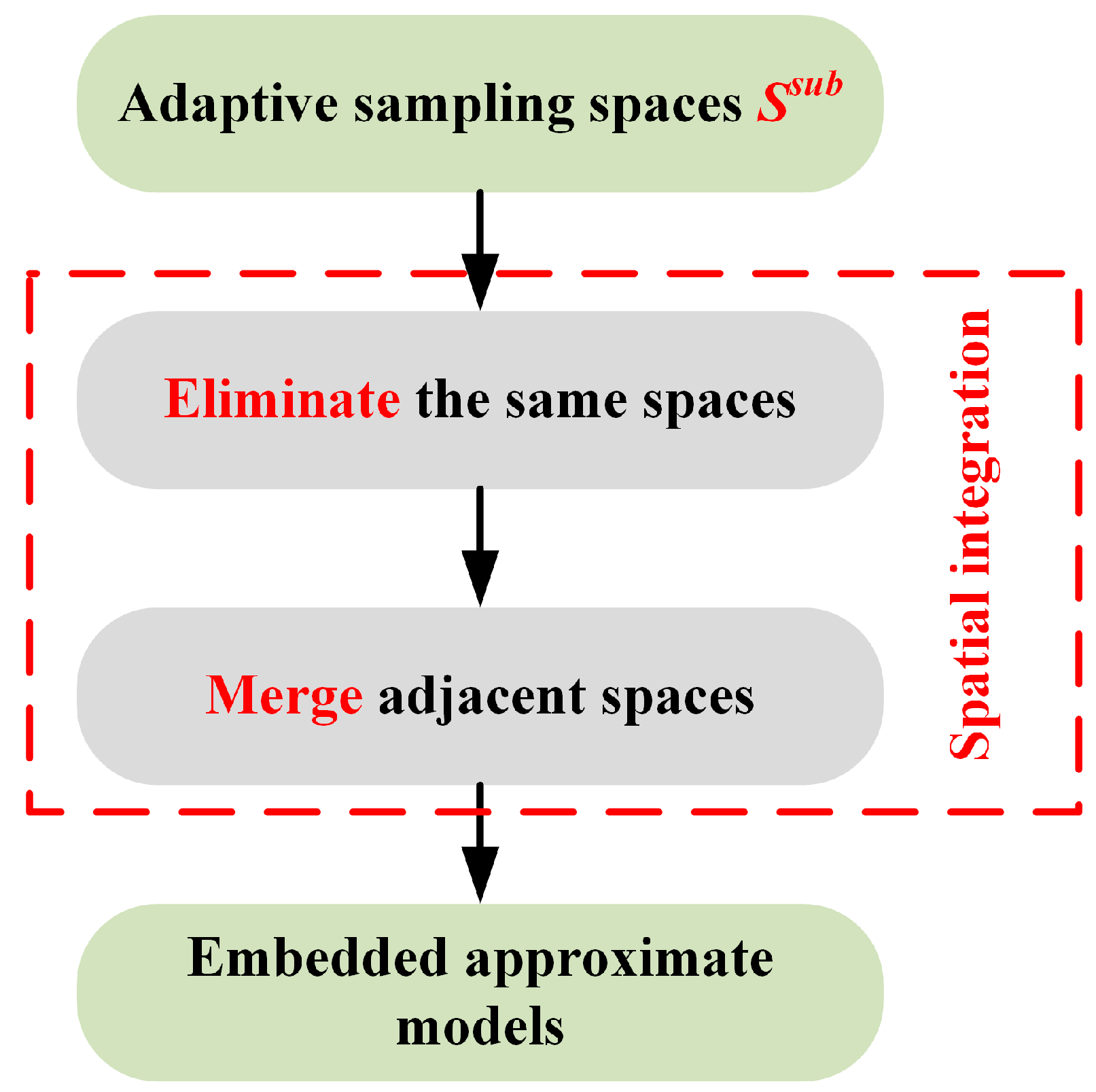
2.2. Embedded Approximate Models

In Section 2.1, the LOO-CV based adaptive sampling directly estimates the prediction errors. In the context of continuous LOO-CV based adaptive sampling, the estimated LOO-CV errors help identify interesting regions for guiding local exploitation in adaptive sampling process [15,29]. However, most of new samples would cluster in a small number of spaces which could lead to overfitting. As shown in Figure 4, based on adaptive sampling, the adaptive sample points are mainly concentrated in the “oscillating region” x ∈ [0, 1.6] on the left, while the “flat region” x ∈ [1.6, 4.0] on the right has little samples. However, the global approximation model obtains an optimal “model” conforming to the characteristics of the “oscillating region” by analysing the samples of the whole design space, which results in the continuation of similar “oscillating” characteristics in the “flat region”.

The mathematical function in Figure 4 is expressed as:

$$f\left(x\right)=\left(\sin \left(7x\right)+\cos \left(14x\right)\right)x^2{e}^{-4x},x\in \left[0,4\right]$$

(6)

It is obvious that the adaptive sample points (Ada-points) of adaptive sampling mainly cluster in the “oscillating region” x ∈ [0, 1.6]. Although this makes the global Kriging approximation model fit well in x ∈ [0, 1.6], serious overfitting phenomenon occurs in the “flat region” x ∈ [1.6, 4.0], which would directly cause the algorithm to miss the optimal solution. To avoid that, a local embedded approximate model construction method is proposed in this section, Figure 5 depicts the flowchart of this method. The major steps are as follows:

(1)

Obtain the centre sample points $x_i^{\mathit{center}}$ of all the sub spaces S^sub;

(2)

Eliminate spaces that have the same center point;

(3)

Calculate the correlation coefficients $R_{ij}^{\mathit{center}}$ between $x_i^{\mathit{center}}$ and $x_j^{\mathit{center}}$; Merge adjacent spaces that the correlation coefficients $R_{ij}^{\mathit{center}}$ ≥ σ (σ = 0.8 in this paper), and;

(4)

Construct local embedded approximation models in the spatial integration regions.

After the construction of dynamic local embedded approximation models (EAM), the model fitting of Equation (4) is shown in Figure 6. The local approximate models (EAM¹, EAM², EAM³ and EAM⁴) are embedded in four different regions respectively, i.e., x ∈ [0, 1.6], x ∈ [0.8, 2.4], x ∈ [1.6, 3.2], and x ∈ [3.2, 4.0], and it can be seen that the EAM fitting effect is well not only in the oscillating region x ∈ [0, 1.6], but also in the other three regions. In fact, the global Kriging approximate model in Figure 4 did not miss the optima during the optimization process, but it is unacceptable for overfitting phenomenon occurred in x ∈ [1.6, 3.2]. This phenomenon cannot be predicted, and in most cases, the algorithm will miss the optima and make the optimization failure, which is not worth the candle. The local embedded approximation models can not only achieve a better fitting in the oscillation or the optimal region, but also explore its local features in the rest of the regions, so that the algorithm can get the actual optima.

Figure 7 depicts the information matrix-based dynamically embedded approximate models process. Firstly, based on the correlation coefficient provided by the information matrix, the sampling spaces with large LOO-CV error points and the optimal point of the current sample set are obtained. Then the construction of the global approximation model is completed until the stopping criterion is met. At the same time, the sampling spaces in the adaptive sampling process are integrated. Finally, the dynamic embedded approximation models are constructed in sampling spaces.

3. Examples

In this section, the superior performance of the proposed the information matrix-based dynamically embedded approximate models method will be examined through seven well-known benchmark optimization problems. All problems are box-constrained and there are no other constraints. Although these seven test problems are not really computationally expensive, they have characteristics typically encountered with black-box global optimization problems and are therefore suitable for assessing the performance of optimization algorithms for computationally expensive problems.

The study consists of two parts. The first one is carried out on two dimensional functions and the second on a high dimensionally scalable problem.

3.1. Two Dimensional Benchmark

In order to reduce the risk of sporadic solutions, based on Latin hypercube design (LHD) [30] method, 50 design of experiments (DOEs) were generated using different seeds. Each of these were used in the optimisation of the tuning parameters for the approximate models.

The five functions in a commonly used test set are displayed as follows:

• Ackley function with two-dimensional (D = 2)

$$f\left(x\right)=-20\exp \left(-0.2\sqrt{\frac{1}{D}{\displaystyle \sum _{i=1}^D{x}_i^2}}\right)-\exp \left(\frac{1}{D}{\displaystyle \sum _{i=1}^D\cos \left(2\pi x_i\right)}\right)+20+\exp \left(1\right),x_i\in \left[-3,3\right]$$

(7)

2.

Alpine function with two-dimensional (D = 2)

$$f\left(x\right)={\displaystyle \sum _{i=1}^D\left|x_i\sin \left(x_i\right)+0.1x_i\right|},x_{1,2,\dots ,D}\in \left[-10,10\right]$$

(8)

3.

Branin-Hoo function (BH) with two-dimensional (D = 2)

$$f\left(x\right)={\left(x_2-5.1x_1^2/4{\pi }^2+5x_1/\pi -6\right)}^2+10\left(1-1/8\pi \right)\cos \left(x_1\right)+10,x_1\in \left[-5,10\right],x_2\in \left[0,15\right]$$

(9)

4.

Griewank function with two-dimensional (D = 2)

$$f\left(x\right)={\displaystyle \sum _{i=1}^D\frac{x_i^2}{4000}}-{\displaystyle \prod _{i=1}^D\cos \left(\frac{x_i}{\sqrt{i}}\right)}+1,x_i\in \left[-10,10\right]$$

(10)

5.

Six-hump Camel-Back (SC) function with two-dimensional (D = 2)

$$f\left(x\right)=\left(4-2.1x_1^2+x_1^4/3\right)x_1^2+x_1{x}_2+\left(-4+4x_2^2\right)x_2^2,x_{1,2}\in \left[-2,2\right]$$

(11)

In this subsection, this study aims to benchmark the information matrix-based dynamically embedded approximate models for different functions. In all tests, the size of the initial sample set m was 5D, the threshold ε of correlation coefficient for adaptive sampling based on information matrix is 0.01, the threshold σ of correlation coefficient based on spatial integration was 0.8, and the maximum iterations I_max for adaptive sampling is set to 10. Computational time is generally proportional to the number of expensive black-box function evaluations for engineering design optimization. Here all benchmark optimization problems are regarded as the computation-intensive models and the objective function values can only be obtained through computation-intensive, black-box computer analysis and simulation. From this viewpoint, the number of function evaluations (NFE) can be used to reflect the computational efficiency. Moreover, the approximate optimum f^∗ is also calculated to reflect the robustness and accuracy of the optimization method. The number of dynamic local embedded approximation models output the optima is denoted by N^EAM. All of the results are shown in

Table 1. The result on five functions.

Fun	Opt(f)	Mean(f∗)	Min(f∗min)	NFE	NEAM
Ackley	0	1.02073	0.05208	40	35
Alpine	0	0.39469	0.00148	40	40
BH	0.39790	0.39798	0.39790	40	1
Griewank	0	0.02073	0.01155	40	33
SC	−1.03163	−1.02454	−1.03163	40	9

.

As shown in Table 1, The global approximation model of IM-DEAM algorithm is not ideal in the optimization of Ackley, Alpine, and Griewank functions, and most of the optima are output by embedded approximation models. It is obvious that the three functions are highly nonlinear on a global scale according to Equations (7), (8) and (10). Therefore, it is not easy to find the optima in the general dynamic global approximation model, and even some regions appear overfitting. However, the local embedded approximate model method can accurately construct the approximate model in the local spaces, so as to accurately explore the local features. For both BH and SC functions, the global approximation model of IM-DEAM can accurately and successfully capture the global optima. It can almost converge to the actual global optimum with a modest number of function evaluations. To describe the superiority of the proposed method further, statistical graphics, i.e., boxplots, are used to show the deviations of the approximate global minima found. The results of the approximate global minima for each run are illustrated in Figure 8 with the help of boxplots.

In Figure 8, the small sizes of boxes imply small standard deviation. It is clear from Figure 8 that the standard deviation of the approximate global minima f^∗ for all test problems is small which implies the robustness of the proposed method. In summary, IM-DEAM reveals the good performance on searching the optimum.

3.2. High Dimensionally Scalable Benchmark

This study aims to benchmark the optimisation techniques for functions with higher dimensionality. This was done using the following dimensionally scalable functions.

• Alpine function with five-dimensional (D = 5)

$$f\left(x\right)={\displaystyle \sum _{i=1}^D\left|x_i\sin \left(x_i\right)+0.1x_i\right|},x_{1,2,\dots ,D}\in \left[-10,10\right]$$

(12)

2.

Griewank function with eight-dimensional (D = 8)

$$f\left(x\right)={\displaystyle \sum _{i=1}^D\frac{x_i^2}{4000}}-{\displaystyle \prod _{i=1}^D\cos \left(\frac{x_i}{\sqrt{i}}\right)}+1,x_i\in \left[-10,10\right]$$

(13)

3.

Trid function (TR) with ten-dimensional (D = 10)

$$f\left(x\right)={\displaystyle \sum _{i=1}^D{\left(x_i-1\right)}^2}-{\displaystyle \sum _{i=2}^D{x}_i{x}_{i-1}},x_i\in \left[-100,100\right]$$

(14)

4.

Sum squares function (SF) with twelve-dimensional (D = 12)

$$f\left(x\right)={\displaystyle \sum _{i=1}^{D}i{x}_i^2},x_i\in \left[-5.12,5.12\right]$$

(15)

In this subsection, the parameter settings for IM-DEAM are the same as in Section 3.1. As with the 2D function, 50 different training DOEs were evaluated for each of the four cases in order to reduce the risk of sporadic solutions.

Table 2. The results on four functions.

Fun	Opt(f)	Mean(f∗)	Min(f∗min)	NFE	NEAM
Alpine	0	2.97921	0.50602	85	48
Griewank	0	0.68073	0.38176	130	45
TR	−210	517.559	−209.903	160	15
SF	0	0.02764	0.00117	190	44

shows the test results of these four functions, and the results of the approximate global minima for each run are illustrated in Figure 9 with the help of boxplots. As shown in Table 2, with the increase of dimension, the role of local embedded approximate model becomes more and more obvious. Most of the optima f^∗ of these three functions i.e., Alpine, Griewank, and SF are provided by local embedded approximation models. Meanwhile, as shown in Figure 9, there are many outliers in TR and SF, especially TR, which makes the mean of the optimal solutions of these two functions larger. In addition to these outliers, the remaining optimal solutions almost converge to the actual global optimum.

Overall, from the accuracy and robustness perspectives, IM-DEAM demonstrates satisfactory performance. It is noted that the proposed method is more accurate and robust than the general optimization methods because of the application of local embedded approximate models.

4. Application to Hull Form Optimisation

In this part, the proposed IM-DEAM is used to optimise the hull form of the David Taylor Model Basin 5415 (DTMB 5415) vessel [31], and the hull surface modification method is the RBF method that is developed by our research group [32]. The CFD simulation experiment is executed by SHIPFLOW. In the following section, the problem is introduced briefly, with results discussed.

4.1. Definition

The hull geometry includes a sonar dome and transom stern. Figure 10 depicts the model and

Table 3. The principal dimensions of the DTMB 5415 model.

Main Principal	Symbol	Value
Length between perpendiculars	Lpp/m	5.719
Designed waterline length	Lw/m	5.726
Moulded breadth	B/m	0.758
Designed draft	T/m	0.248
Wetted surface area	SW/m2	4.865
Displacement volume	∇/m3	0.550
Block coefficient	CB	0.505
Wave-making resistance	CW/10−3	0.918

lists the major parameters of the model. The objective function is described by the following:

$$\begin{array}{l}\mathrm{Min}{f}_{obj}=C_W,F_r=0.28\\ st.\frac{\left|{\nabla }_{opt}-\nabla \right|}{\nabla }\le 1\%\end{array}$$

(16)

where C_W is the wave making resistance coefficient; and ∇ and ∇_opt are the displacement volumes of the original and optimised models, respectively.

Through design experience, a total of 11 variable points were selected as design variables. All of the control points are distributed on the forebody, as the forebody is crucial for the wave resistance. Figure 11 depicts the locations of these variable points.

Table 4. Settings for design variables.

	Y1	Y2	X3	Y4	Y5	Y6	Y7	Y8	Y9	Y10	Y11
Upper limit	0.240	0.150	0.400	0.037	0.030	0.160	0.060	0.095	0.065	0.160	0.115
Lower limit	0.200	0.120	0.200	0.012	0.020	0.100	0.040	0.050	0.038	0.150	0.090
Initial value	0.227	0.134	0.395	0.014	0.026	0.120	0.055	0.086	0.049	0.154	0.105

lists the initial values and ranges of values of the design variables. The location of variable point X₃ was allowed to vary along the direction of the hull length; the locations of the remaining ten variable points were allowed to vary along the direction of the hull width. Specifically, Y₁, Y₅, Y₈, and Y₁₀ were located near the waterline and were responsible for controlling the shape of the waterline at the entrance of the ship. Y₂, Y₄, Y₇, and Y₁₁ were located on the bilge of the hull and were responsible for controlling the profile of the bilge at the entrance of the ship. Variable points X₃, Y₆, and Y₉ were used to vary the length and width of the dome bow; the remaining parameters were used to vary the body line and waterline geometries at the corresponding locations.

4.2. IM-DEAM

In this optimization, 60 initial sample points were sampled in the design space to obtain a set of initial sample set by LHD. Subsequently, the wave-making resistance $C_W^i$ (i = 1, …, 60) of each sample. The threshold ε of correlation coefficient for adaptive sampling based on information matrix is 0.01, the threshold σ of correlation coefficient based on spatial integration was 0.8, and the maximum iterations I_max for adaptive sampling is set to 10. Optimisation results are shown in

Table 5. The optimization results of the DTMB 5145.

	${\mathit{C}}_{\mathit{W}}^{\mathbf{\ast }}$	CW	Y1	Y2	X3	Y4	Y5	Y6	Y7	Y8	Y9	Y10	Y11
GAM	0.364 × 10−3	0.621 × 10−3	0.216	0.150	0.200	0.028	0.026	0.152	0.040	0.082	0.038	0.160	0.115
EAM	0.382 × 10−3	0.419 × 10−3	0.221	0.137	0.291	0.031	0.023	0.129	0.048	0.059	0.057	0.156	0.093
	Upper limit		0.239	0.149	0.348	0.035	0.029	0.154	0.059	0.094	0.063	0.160	0.112
	Lower limit		0.201	0.121	0.200	0.012	0.020	0.101	0.040	0.054	0.038	0.151	0.090

. In Table 5, the optima of the global approximate model (GAM) and local embedded approximate model (EAM) of IM-DEAM are presented respectively. Each simulation was performed on a single core of an Intel Core i7-8700 processor at 3.19 GHz.

As shown in Table 5, due to the complexity of hull form optimization, the uneven distribution of sample points in the process of adaptive sampling led to the over-fitting of the global approximation model of IM-DEAM. This makes the predicted value of the optimal wave-making resistance $C_W^{\ast }$ of the global approximation model (GAM) deviate greatly from the actual wave-making resistance C_W. However, the EAM is constructed by establishing a local approximation model in the integrated subspace with 86 sample points, which alleviates over-fitting well and finds the optimal solution successfully.

4.3. Results

According to the results in Table 5, we choose the optimal solution of EAM as the final optimal hull form.

Table 6. Performance comparison of initial and optimized hull form.

	Ini	Opt	Variation
Displacement volume/m3	0.550	0.554	+0.73%
Wetted surface area/m2	4.865	4.929	+1.32%
CW/10−3	0.918	0.419	−54.36%
Total resistance RT/N	22.091	19.410	−12.14%

shows the final results comparison of initial and optimized hull form. It can be seen that the optimised hull form leads to 0.73% increase in displacement volume and a large decrease (54.36%) in wave-making resistance. The total resistance performance R_T could be calculated using the viscous flow CFD software STAR-CCM+. As a result, the total resistance of the optimized hull form is reduced by 12.14%.

Figure 12 depicts a comparison of the bow geometries of the initial and optimised hull forms. Figure 13 depicts a comparison of the corresponding wave patterns and wave cuts. As depicted in Figure 12, the optimised hull form has a concave surface near the waterline at the bow, narrowing the designed waterline and changing the geometry below the waterline from more V-shaped to more U-shaped. In addition, the shape of the dome bow becomes markedly longer and wider. As depicted in Figure 13, with the geometries of the bow and dome bow optimised, the wave height at the bow decreases, leading to constructive interferences at the entrance and a markedly decreased wave height at the midships. This aspect is conducive to decreasing the wave making resistance, finally leading to 54.36% decrease in the wave-making resistance coefficient of the optimised hull form. Because the hull resistance is positively proportional to the wet surface area, as listed in Table 6, the hull form optimisation results in a 1.32% increase in the wet surface area and 0.73% increase in the displacement volume, finally, 12.14% decrease in the total resistance. Figure 14 shows the comparisons of wave-making resistance coefficients in a wide range of speed between initial and optimal hull form. It can be seen that the wave-making resistance of the optimized hull form is reduced at different speeds. As a whole, IM-DEAM algorithm can efficiently deal with hull form optimization problems.

5. Conclusions

In this study, a method was proposed for the identification and dynamic sampling of subspaces based on the sample information matrix. The method effectively balances the efficiency of the search and accuracy of optima. In addition, local approximate models are embedded in subspaces identified, thereby preventing the overfitting caused by a dense distribution of samples. This assists the algorithm in optimisation and improves the reliability and robustness of the optima. The IM-DEAM method was validated by using it to optimise mathematical problems and the geometry of hull model DTMB 5415 to confirm its reliability, robustness, and wider applications. The major contributions of the IM-DEAM method proposed in this study are summarised as follows:

(1)

Adaptive sampling is performed by fully utilising the Gaussian-function information matrix and adaptively extracting subspaces with significant LOO-CV errors and potential optimum subspaces. In other words, subspaces with two different natures are considered simultaneously to improve the efficiency of additional sampling and explore optimum information.

(2)

Local approximate models are embedded in subspaces, thereby preventing the overfitting and spurious optima of global approximate models caused by an excessively concentrated sample distributions. In addition, the embedded local approximate models assist in global optimisation, thereby improving the reliability of optima.

However, the IM-DEAM method has some deficiencies. First, for problems with very complex target spaces, the local uniformity of the additional points sampled using the LHD method needs to be improved. Next, embedded approximate models can assist global approximate models in optimisation; however, in highly nonlinear, complex spaces, there is a lack of criteria for evaluating the quality of the global and local optima. Finally, the accuracy of embedded approximate models decreases owing to the size of subspaces and the scarcity of sample points in higher dimensions. Therefore, further research is required to address the problems of an inadequate number of samples during the building of embedded approximate models and many local optima in the target space.

It is well known that a ship is a complex system. With the development of multi-objective decision making (MODM), multi-criteria decision-making (MCDM), and multi-attribute decision making (MADM) optimization [8,33], the focus of hull form optimization will be multi-constraint and multi-objective in the future work.

References

- Andrić, J.; Kitarović, S.; Bičak, M. IACS incremental-iterative method in progressive collapse analysis of various hull girder structures. Brodogradnja Teorija i Praksa Brodogradnje i Pomorske Tehnike 2014, 65, 65–77. [Google Scholar]
- Andrić, J.; Prebeg, P.; Andrisic, J.; Žanić, V. Structural optimisation of a bulk carrier according to IACS CSR-BC. Ships Offshore Struct. 2020, 15, 123–137. [Google Scholar] [CrossRef]
- Andrić, J.; Prebeg, P.; Pala:ersa, M.; Žanić, V. Influence of different topological variants on optimized structural scantlings of passenger ship. Mar. Struct. 2021, 78, 102981. [Google Scholar] [CrossRef]
- Prebeg, P.; Zanic, V.; Vazic, B. Application of a surrogate modeling to the ship structural design. Ocean Eng. 2014, 84, 259–272. [Google Scholar] [CrossRef]
- Nouri, N.M.; Mohammadi, S.; Zarezadeh, M. Optimization of a marine contra-rotating propellers set. Ocean Eng. 2018, 167, 397–404. [Google Scholar] [CrossRef]
- Koch, P.N.; Simpson, T.W.; Allen, J.K.; Mistree, F. Statistical approximations for multidisciplinary design optimization: The problem of size. J. Aircr. 1999, 36, 275. [Google Scholar] [CrossRef]
- Prebeg, P.; Žanić, V.; Važić, B. An application of a complex system optimization techniques to the ship structural design. In Proceedings of the 11th International Marine Design Conference 2012, Glasgow, UK, 11–14 June 2012. [Google Scholar]
- Žanić, V.; Andrić, J.; Prebeg, P. Design synthesis of complex ship structures. Ships Offshore Struct. 2013, 8, 383–403. [Google Scholar] [CrossRef] [Green Version]
- Liu, H.; Ong, Y.-S.; Cai, J. A survey of adaptive sampling for global metamodeling in support of simulation-based complex engineering design. Struct. Multidiscip. Optim. 2017, 57, 393–416. [Google Scholar] [CrossRef]
- Chang, H.; Cheng, X.; Liu, Z.; Feng, B.; Zhan, C. Sample selection method for ship resistance performance optimization based on approximated model. J. Ship Res. 2016, 60, 1–13. [Google Scholar] [CrossRef]
- Grosso, A.; Jamali, A.; Locatelli, M. Finding maximin latin hypercube designs by Iterated Local Search heuristics. Eur. J. Oper. Res. 2009, 197, 541–547. [Google Scholar] [CrossRef]
- Gorissen, D.; Crombecq, K.; Hendrickx, W.; Dhaene, T. Adaptive distributed metamodeling. In Proceedings of the International Conference on High Performance Computing for Computational Science; Rio de Janeiro, Brazil, 10–13 June 2006, Springer: Berlin/Heidelberg, Germany, 2006; pp. 579–588. [Google Scholar]
- Settles, B. Active Learning Literature Survey; University of Wisconsin: Madison, WI, USA, 2010. [Google Scholar]
- Peri, D. Insean Self-Learning Metamodels for Optimization. Ship Technol. Res. 2009, 56, 95–109. [Google Scholar] [CrossRef]
- Jiang, P.; Shu, L.; Zhou, Q.; Zhou, H.; Shao, X.; Xu, J. A novel sequential exploration-exploitation sampling strategy for global metamodeling. IFAC-PapersOnLine 2015, 48, 532–537. [Google Scholar] [CrossRef]
- Beck, J.; Guillas, S. Sequential design with mutual information for computer experiments (MICE): Emulation of a tsunami model. SIAM/ASA J. Uncertain. Quantif. 2016, 4, 739–766. [Google Scholar] [CrossRef] [Green Version]
- Xu, S.; Liu, H.; Wang, X.; Jiang, X. A robust error-pursuing sequential sampling approach for global metamodeling based on voronoi diagram and cross validation. J. Mech. Des. 2014, 136, 071009. [Google Scholar] [CrossRef]
- Zhu, Z.; Du, X. Reliability analysis with monte carlo simulation and dependent kriging predictions. J. Mech. Des. 2016, 138, 121403. [Google Scholar] [CrossRef]
- Ye, P.; Pan, G. Global optimization method using ensemble of metamodels based on fuzzy clustering for design space reduction. Eng. Comput. 2017, 33, 573–585. [Google Scholar] [CrossRef]
- Yu, H.; Tan, Y.; Sun, C.; Zeng, J. A generation-based optimal restart strategy for surrogate-assisted social learning particle swarm optimization. Knowl. Based Syst. 2019, 163, 14–25. [Google Scholar] [CrossRef]
- Li, C.; Fang, H.; Gong, C. Development of an efficient global optimization method based on adaptive infilling for structure optimization. Struct. Multidiscip. Optim. 2020, 62, 3383–3412. [Google Scholar]
- Yu, M.; Li, X.; Liang, J. A dynamic surrogate-assisted evolutionary algorithm framework for expensive structural optimization. Struct. Multidiscip. Optim. 2020, 61, 711–729. [Google Scholar] [CrossRef]
- Cai, X.; Qiu, H.; Gao, L.; Jiang, C.; Shao, X. An efficient surrogate-assisted particle swarm optimization algorithm for high-dimensional expensive problems. Knowl. -Based Syst. 2019, 184. [Google Scholar] [CrossRef]
- Chang, H.; Zhan, C.; Liu, Z.; Cheng, X.; Feng, B. Dynamic sampling method for ship resistance performance optimisation based on approximated model. Ships Offshore Struct. 2021, 16, 386–396. [Google Scholar] [CrossRef]
- Žanić, V.; Čudina, P. Multiattribute decision making methodology in the concept design of tankers and bulk carriers. Brodogradnja Teorija i Praksa Brodogradnje i Pomorske Tehnike 2009, 60, 19–43. [Google Scholar]
- Lophaven, S.N.; Nielsen, H.B.; Søndergaard, J. DACE: A Matlab Kriging Toolbox; IMM, Informatics and Mathematical Modelling; The Technical University of Denmark: Copenhagen, Denmark, 2002; Volume 2. [Google Scholar]
- Farhang-Mehr, A.; Azarm, S. Bayesian meta-modelling of engineering design simulations: A sequential approach with adaptation to irregularities in the response behaviour. Int. J. Numer. Methods Eng. 2005, 62, 2104–2126. [Google Scholar] [CrossRef]
- Viana, F.; Haftka, R.T.; Steffen, V. Multiple surrogates: How cross-validation errors can help us to obtain the best predictor. Struct. Multidiscip. Optim. 2009, 39, 439–457. [Google Scholar] [CrossRef]
- Aute, V.; Saleh, K.; Abdelaziz, O.; Azarm, S.; Radermacher, R. Cross-validation based single response adaptive design of experiments for Kriging metamodeling of deterministic computer simulations. Struct. Multidiscip. Optim. 2013, 48, 581–605. [Google Scholar] [CrossRef]
- Wang, G.G. Adaptive response surface method using inherited latin hypercube design points. J. Mech. Des. 2003, 125, 210–220. [Google Scholar] [CrossRef]
- Wu, J.; Liu, X.; Zhao, M.; Wan, D. Neumann-Michell theory-based multi-objective optimization of hull form for a naval surface combatant. Appl. Ocean Res. 2017, 63, 129–141. [Google Scholar] [CrossRef]
- Feng, B.; Feng, M.; Chang, H.; Zhang, L. Application of surface deformation method based on radial basis interpolation in multi-objective optimization of ship hull. JSCUT Nat. Sci. Ed. 2019, 47, 128–136. [Google Scholar]
- Andrić, J.; Prebeg, P.; Žanić, V. Multi-level Pareto supported design methodology- application to RO-PAX structural design. Mar. Struct. 2019, 67, 102638. [Google Scholar] [CrossRef]