Application of Improved Particle Swarm Optimisation Algorithm in Hull form Optimisation

Abstract

The particle swarm optimisation (PSO) algorithm has been widely used in hull form optimisation owing to its feasibility and fast convergence. However, similar to other intelligent algorithms, PSO also has the disadvantages of local premature convergence and low convergence performance. Moreover, optimization data are not used to analyse and reduce the range of values for relevant design variables. Our study aimed to solve these existing problems in the PSO algorithm and improve PSO from four aspects, namely data processing of particle swarm population initialisation, data processing of iterative optimisation, particle velocity adjustment, and particle cross-boundary configuration, in combination with space reduction technology. The improved PSO algorithm was used to optimise the hull form of an engineering vessel at Fn = 0.24 to reduce the wave-making resistance coefficient under static constraints. The results showed that the improved PSO algorithm could effectively improve the optimisation efficiency and reliability of PSO and effectively overcome the drawbacks of the PSO algorithm.

1. Introduction

With the continuous improvement of computer processing power and the accuracy of computational fluid dynamics (CFD), CFD-based hull form optimisation has been rapidly developed. This directly applies hull surface parametric modification, CFD numerical simulations, and optimisation technologies to the design of new ships and eventually obtains the hull form with the best performance under given constraints. Many scholars have carried out considerable research on hull form optimisation, including D. Peri [1,2] of Italian Ship Model Basin, Rome; S. Harries [3] of the Technische Universität Berlin; Yang C [4,5,6] of George Mason University, USA; and Feng Baiwei [7,8,9] and Chang Haichao et al. [10,11,12] of Wuhan University of Technology.

At present, the research pertaining to hull form optimisation includes the following. (1) Design space reduction. Harries and Abt [13] reported a massive reduction of parameters that spanned the design space and utilized the gradient information as derived from adjoint simulations. D’Agostino et al. [14] and Serani et al. [15] reduced the dimensionality of the design space by providing a shape reparameterization using Karhunen–Loeve expansion/principal component analysis (KLE/PCA) eigenvalues and eigenmodes. Khan et al. [16] adopted a two-step learning methodology to identify a lower-dimensional latent space based on the combination of geometry- and physics-informed principal component analysis and active subspace method, which can be utilized for efficient design exploration and the construction of improved surrogate models for physics-based prediction of designs. Tezzele et al. [17] pioneered the application of a methodology based on active subspace properties to the naval architecture field for parameter space reduction. (2) Metamodel. Serani et al. [18] reported a study on four adaptive sampling methods of a multi-fidelity metamodel, based on stochastic radial basis functions (RBFs), to achieve a global design optimisation using expensive CFD computer simulations and adaptive grid refinement. Chunna et al. [19] proposed an effective global optimisation method that integrates the adaptive filling algorithm based on fuzzy clustering into the kriging model. Zhang et al. [20] proposed a data prediction method based on improved particle swarm optimisation (IPSO)-Elman NN to improve the prediction accuracy of total resistance. Coppedè et al. [21] proposed a Gaussian process-response surface method (GP-RSM) based on an ordinary kriging model, which was developed to enhance the evaluation speed of the quantity of interest in the design process and applied to improve the calm-water performance of the KCS. (3) Efficient optimisation algorithm. Pellegrini et al. [22] proposed a multi-objective derivative-free and deterministic global/local hybrid algorithm as an efficient and effective solution to SBDO problems. Tezdogan et al. [23] proposed a hybrid algorithm to solve the complicated nonlinear optimisation problem of fishing boat. Serani et al. [24] presented study of DPSO, with application to simulation-based design in ship hydrodynamics. Leotardi [25] describes a class of novel initializations in deterministic particle swarm optimization (DPSO) for approximately solving costly unconstrained global optimization problems.

Owing to the complex spatial characteristics of hull form design optimisation, a general mathematical method cannot provide feasible solutions in the actual optimisation process. Therefore, intelligent optimisation algorithms, such as a genetic algorithm (GA) or particle swarm optimisation (PSO), are used in hull form optimisation to obtain approximately optimal solutions. PSO is a population-based stochastic optimisation technique introduced by Kennedy and Eberhart in 1995 [26,27]. The PSO algorithm is easier to implement, has fewer parameters, and has proven to converge faster than conventional optimisation methods such as GA [28,29]. Owing to its simplicity, ease of implementation, and high convergence speed [30,31], the PSO algorithm has been widely used for hull form optimisation.

Similar to other intelligent optimisation algorithms, the PSO algorithm also exhibits the disadvantages of local premature convergence and low convergence performance. To solve such problems, many scholars have improved PSO. Because the PSO algorithm falls into local optimisation in high-dimensional problems, Cheng et al. [30] modified the particle diversity in the optimisation process to improve the optimisation performance. Mathew M. Noel [31] combined PSO with the gradient algorithm to increase the local optimisation ability, thereby improving the algorithm optimisation efficiency and optimisation progress. Shi et al. [32] made a comprehensive improvement on the inertial weight adjustment strategy, differential evolution, and local variable depth search of PSO, which reasonably and efficiently balanced the global and local search abilities of the algorithm. Reungsinkonkarn et al. [33] applied search space reduction (SSR) to PSO to eliminate the optimal region that may not find the optimal solution through SSR and to improve the algorithm optimisation efficiency. Zhang et al. [34] proposed a multi-objective discrete PSO algorithm based on a fine perturbation strategy (EPSMODPSO), which performs well in the diversity and convergence of the obtained Pareto optimal frontier. It can reconfigure the ship power system and solve other multi-objective discrete optimisation problems. To improve the premature convergence and low search accuracy of conventional PSO, Wang et al. [35] proposed PSO with an enhanced global search and local search (EGLPSO) to improve global and local search. This algorithm can greatly improve the performance of conventional PSO in terms of search accuracy, search efficiency, and global optimality.

Our study achieved certain improvement of the PSO algorithm in terms of its existing problems. In the process of particle initialisation and optimisation iteration, the space reduction method was introduced to reduce the particle-changing space in the optimisation process. The particle velocity and the cross-boundary particles after space reduction were processed to improve the particle diversity in the optimisation process. The method was verified by function examples. The results showed that the improved algorithm can improve the optimisation efficiency while ensuring the optimisation performance. Finally, the improved PSO algorithm was applied to the hull form optimisation of an engineering vessel.

This article has five sections. Section 2 introduces the space reduction technique. Section 3 describes the improved PSO algorithm. Section 4 verifies the feasibility of the improved optimisation algorithm by function examples. Section 5 applies this algorithm to the optimisation of the bow shape of a certain engineering ship. Section 6 summarises the research and describes the future directions.

2. Space Reduction Technique Based on Partial Correlation Analysis

Space reduction is a practical division and reduction of the design space through exploration and analysis, including dimensional reduction and size reduction. Hull form optimisation is a typical and complex engineering problem. It contains a large amount of numerical simulation with complex spatial design performance, leading to low optimisation efficiency and difficulty in obtaining global optimal solutions. To improve its efficiency and performance, many scholars have introduced space reduction into hull form optimisation [8,36]. In our study, we used the partial correlation analysis for design space reduction.

2.1. Partial Correlation Analysis

A correlation coefficient symmetry matrix composed of simple coefficients is required to calculate the partial correlation coefficient [37,38]. There are n variables X₁, X₂, …, X_n, the Pearson correlation coefficient between any two variables X_i, X_j is r_ij(i, j = 1, 2, …, n), and the Pearson correlation coefficient is calculated as

$$r_i{}_j=\frac{{\displaystyle \sum (X_i-{\overline{X}}_i)(X_j-{\overline{X}}_j)}}{\sqrt{{\displaystyle \sum {(X_i-{\overline{X}}_i)}^2{(X_j-{\overline{X}}_j)}^2}}}$$

(1)

where $\overline{X}$ is the average. The following correlation coefficient symmetry matrix is composed of simple correlation coefficients:

$$R=\left[\begin{array}{cccc}{r}_{11}& r_{12}& \dots & r_{1n}\\ r_{21}& r_{22}& \dots & r_{2n}\\ \dots & \dots & \dots & \dots \\ r_{n1}& r_{n2}& \dots & r_{nn}\end{array}\right]$$

(2)

The partial correlation coefficient between any two variables X_i and X_j is R_ij, and the equation for calculating the partial correlation coefficient is

$$R_{ij}=\frac{-{\Delta }_{ij}}{\sqrt{{\Delta }_{ii}\cdot {\Delta }_{ii}}}$$

(3)

where ${\Delta }_{ij}$, ${\Delta }_{ii}$, and ${\Delta }_{jj}$ are algebraic cofactors corresponding to elements r_ij, r_ii, and r_jj in in the symmetric matrix of the correlation coefficient, respectively.

The correlation coefficient between variables and objectives can be obtained with appropriate data samples using the above theory. A positive sign before the partial correlation coefficient represents a positive linear relationship between the variable and the target; the negative sign represents a negative linear relationship between the variable and the target; the distribution range of the coefficient is between 0 and 1; and the numerical value indicates the linear correlation between the design variable and the target. The feasibility study of partial correlation analysis for space reduction is detailed in Wu’s article [36].

2.2. Partial Correlation Coefficient and Degree-of-Space Reduction

The relationship between the value of the partial correlation coefficient and the spatial distribution of variables is investigated by using a single objective function. Equation (4) is used in the first step.

$$y=\left|x\right|$$

(4)

When $x\in \left[0,1\right]$, the relationship between the target and variable is as shown in Figure 1. The figure shows that there is a positive linear relationship between the target and the variable. When $x=0$, the minimum value of the function $y=0$ is obtained. The distribution space of x is divided into two equal parts; (0, 0.5) is defined as the lower space, (0.5, 1) is the upper space, and x = 0.5 is the median of the variable, which is the midpoint of the x distribution space. Fifty random samplings are performed to calculate the function values and perform partial correlation analysis. The obtained partial correlation coefficient between y and x is 1. It is concluded that the smaller the value of x, the is smaller the value of y. Therefore, the upper space of the x variable is irrelevant for obtaining the minimum value of the function and can be discarded.

When $x\in \left[-1,1\right]$, the relationship between the target and the variable is as shown in Figure 2. It is impossible to analyse the correlation between the variable and the function value from the overall space of the variable. Similarly, the distribution space of x is divided into two equal parts. When x is the variable median value x = 0, the function value is smallest. One hundred samplings are randomly to calculate the function values and perform partial correlation analysis. The obtained partial correlation coefficient between y and x is 0.0055. Theoretically, the partial correlation coefficient obtained by uniform sampling in the variable space should be 0. The resulting partial correlation coefficient is a value close to 0 owing to random sampling. Therefore, it is impossible to determine whether the upper and lower spaces are valuable for obtaining the minimum value of the function, and these spaces cannot be discarded.

The function with the local maximum value (Equation (5)) is selected for further study. The relationship between the target and variable is as shown in Figure 3. The characteristic of this function is that there are many local optimal solutions, and the minimum value y = 0 is obtained when x = 0, which is closer to the actual optimisation than Equation (4).

$$y=\sin (x^2)+\left|x\right|$$

(5)

The function is randomly sampled 1000 times in different variable ranges, and a partial correlation analysis is performed. The results are shown in

Table 1. Function analysis results.

Range of x	[−5,5]	[−4,5]	[−3,5]	[−2,5]	[−1,5]	[0,5]
Variable median	x = 0	x = 0.5	x = 1	x = 1.5	x = 2	x = 2.5
Optimal value	x = 0
Partial correlation coefficient	−0.021	0.260	0.524	0.736	0.872	0.894

. By testing the ranges of different x values, it can be found that when the optimal value is the median of the variable, the partial correlation coefficient is close to 0; when the optimal value is farther from the median of the variable and is closer to the boundary value of a side, the partial correlation coefficient is close to 1. Similarly, it can be concluded that when the partial correlation coefficient is 0, the space on both sides of the median value cannot be discarded; when the partial correlation coefficient is 1, the space on one side can be discarded by determining the sign of the partial correlation coefficient.

Therefore, the relationship between the partial correlation coefficient and spatial reduction is defined as follows: when the partial correlation coefficient is 0, the variable space is not reduced, and the space reduction is 0% of the initial space; when the partial correlation coefficient is 1, the upper (lower) space is abandoned, and the space reduction is 50% of the initial space.

3. Improved Particle Swarm Optimisation

3.1. Particle Swarm Optimisation

In the PSO algorithm, each particle contains three pieces of information: velocity, location, and fitness. Of these, the velocity information determines the direction change of a particle; the location information contains the applicable values of parameters; the fitness represents the performance of a particle. The updated equations of particle velocity and particle position are shown in Equations (6) and (7), respectively.

$$v_j^i=w\cdot v_j^{i-1}+c_1{r}_1(pbes{t}_j-p_j^{i-1})+c_2{r}_2(gbest-p_j^{i-1})$$

(6)

$$p_j^i=p_j^{i-1}+v_{{}^j}^i$$

(7)

where $v_j^i$ is the velocity of the i-th generation, j-th particle; $p_j^i$ is the position of the i-th generation, j-th particle; w is the weighting factor, whose magnitude affects the inertia of the particle flight; c₁ and c₂ are learning factors, affecting the local and global fusion effect, respectively; r₁ and r₂ represent random numbers from 0 to 1; Pbest represents the optimal position information of the particles and records the optimal position of individual particles; and gbest represents the global optimal position information and records the optimal position of the particle group. In our PSO algorithm, the value of w was 0.8; c₁ = c₂ = 2.

3.2. Improvement of Particle Swarm Optimisation

In this study, the PSO algorithm is improved with respect to data processing of particle swarm population initialisation, data processing of iterative optimisation, particle velocity adjustment, and particle cross-boundary configuration.

3.2.1. Data Processing of Particle Swarm Population Initialisation

The PSO algorithm generally uses Equation (8) for particle initialisation [26,39,40].

$$\left\{\begin{array}{l}{p}_j^0=rand\times (p_{\max }-p_{\min })+p_{\min }\\ v_j^0=rand\times (v_{\max }-v_{\min })+v_{\min }\end{array}\right.$$

(8)

where rand is a random number uniformly distributed between 0 and 1; p_max and p_min are the upper and lower boundary values of the particle position component, respectively; and v_max and v_min are the upper and lower boundary values of the particle velocity component, respectively.

Figure 4 illustrates the examples of random sampling applied to the 6-dimensional and 10-dimensional optimization problems, wherein two variables are selected for two-dimensional (2D) projection. We observed that data clustering or data omission existed in the sample space. Furthermore, uniform design (UD) was used to improve the initialization of the PSO algorithm to ensure uniformity of the initial particles in the space.

UD, proposed by Fang [41] in China, is an experimental design method developed using the uniform distribution theory. In the uniform test, the level of each factor was evenly distributed within the test range, and each level was tested only once. Figure 5 depicts the projection of the sample points generated by the UD on a two-dimensional plane. We observed that the distribution of sample points was uniform regardless of the dimensionality of the design variables.

3.2.2. Data Processing of Particle Iterative Optimisation

The optimisation data in the iterative optimisation process also contain many hidden relationships that cannot be visually displayed. The optimisation process could generate a large amount of data. The analysis of these data can provide guidance to the subsequent particle optimisation, making the particles quickly cluster into a space worth exploring. So, this study used partial correlation analysis to perform datamining on the particles and the fitness values and thus obtain their relationships and complete the reduction of the initial search space of the particles. The partial correlation coefficient was calculated by Equations (1)–(3). According to the conclusions drawn in Section 2.2, when the partial correlation coefficient is set to 0, the range of the relevant design variables is not reduced; when the partial correlation coefficient is 1, the values of the relevant design variables are 50% of those in the initial range. In this article, two different methods are proposed to establish the relationship between the partial correlation coefficient and the degree of space reduction, which are the segmentation function reduction method as shown in

Table 2. Partial correlation coefficient and space reduction.

Rij (Absolute Value)	0.00–0.05	0.05–0.15	0.15–0.25	0.25–0.35	0.35–0.45	0.45–0.55	0.55–0.65	0.65–0.75	0.75–0.85	0.85–0.95	0.95–1.00
Coerp	0%	5%	10%	15%	20%	25%	30%	35%	40%	45%	50%

and the linear function reduction method as shown in Equation (9), where, R_ij represents the partial correlation coefficient, and Coe_rp represents the degree-of-space reduction.

Coe_rp = 50% × R_ij

(9)

3.2.3. Particle Velocity Adjustment Strategy

As the particle search space changes, the speed of the particle swarm must be adjusted accordingly.

In the PSO algorithm, the upper and lower boundaries of the velocity are calculated by Equation (10), and the boundary values remain unchanged during the entire optimisation process. In this study, the value of n is 5.

$$\left\{\begin{array}{c}{v}_{\max }=(p_{\max }-p_{\min })/n\\ v_{\min }=-(p_{\max }-p_{\min })/n\end{array}\right.\begin{array}{c} n \mathrm{is} \mathrm{a} \mathrm{positive} \mathrm{integer}\end{array}$$

(10)

The upper and lower boundaries of the velocity determine the accuracy of the area between the current position and the optimal position. If the velocity is too high, it may cause the particles to cross the optimal space. If it is too low, it may cause the particles to fall into a local optimum. Therefore, as the search space continues to decrease, the upper and lower boundaries of the particle velocity should change correspondingly with the search space. The upper and lower boundary values of the particle velocity in the optimisation process are modified as Equation (11).

$$\left\{\begin{array}{c}{v}_{\max }^i=(p_{\max }^i-p_{\min }^i)/n\\ v_{\min }^i=-(p_{\max }^i-p_{\min }^i)/n\end{array}\right.\begin{array}{c} n \mathrm{is} \mathrm{a} \mathrm{positive} \mathrm{integer}\end{array}$$

(11)

where $v_{\max }^i$ and $v_{\min }^i$ represent the optimisation velocity of the upper and lower boundaries in the i-th generation, and $p_{\max }^i$ and $p_{\min }^i$ represent the upper and lower boundary values of the particle position components in the i-th generation, respectively.

3.2.4. Particle Cross-Boundary Configuration

Because the search space of the particles is reduced during the optimisation process, the position and velocity of the particles often cross the upper and lower boundaries. In the PSO algorithm, these particles are set as the boundary values to resolve this problem. To give the particles better ability to explore the optimal solution in the reduced search space, our study configured the cross-boundary particles as shown in Equation (12).

$$\left\{\begin{array}{l}{p}_{\mathrm{over}}^i=rand\times (p_{\max }^i-p_{\min }^i)+p_{\min }^i\\ v_{\mathrm{over}}^i=rand\times (v_{\max }^i-v_{\min }^i)+v_{\min }^i\end{array}\right.$$

(12)

where $p_{over}^i$ and $v_{over}^i$ represent the position and velocity of the i-th generation cross-boundary particle; $v_{\max }^i$ and $v_{\min }^i$ represent the optimisation speed of the upper and lower boundaries of the i-th generation; $p_{\max }^i$ and $p_{\min }^i$ represent the upper and lower boundary values of the particle position components in the i-th generation, respectively; and rand is a random number between 0 and 1.

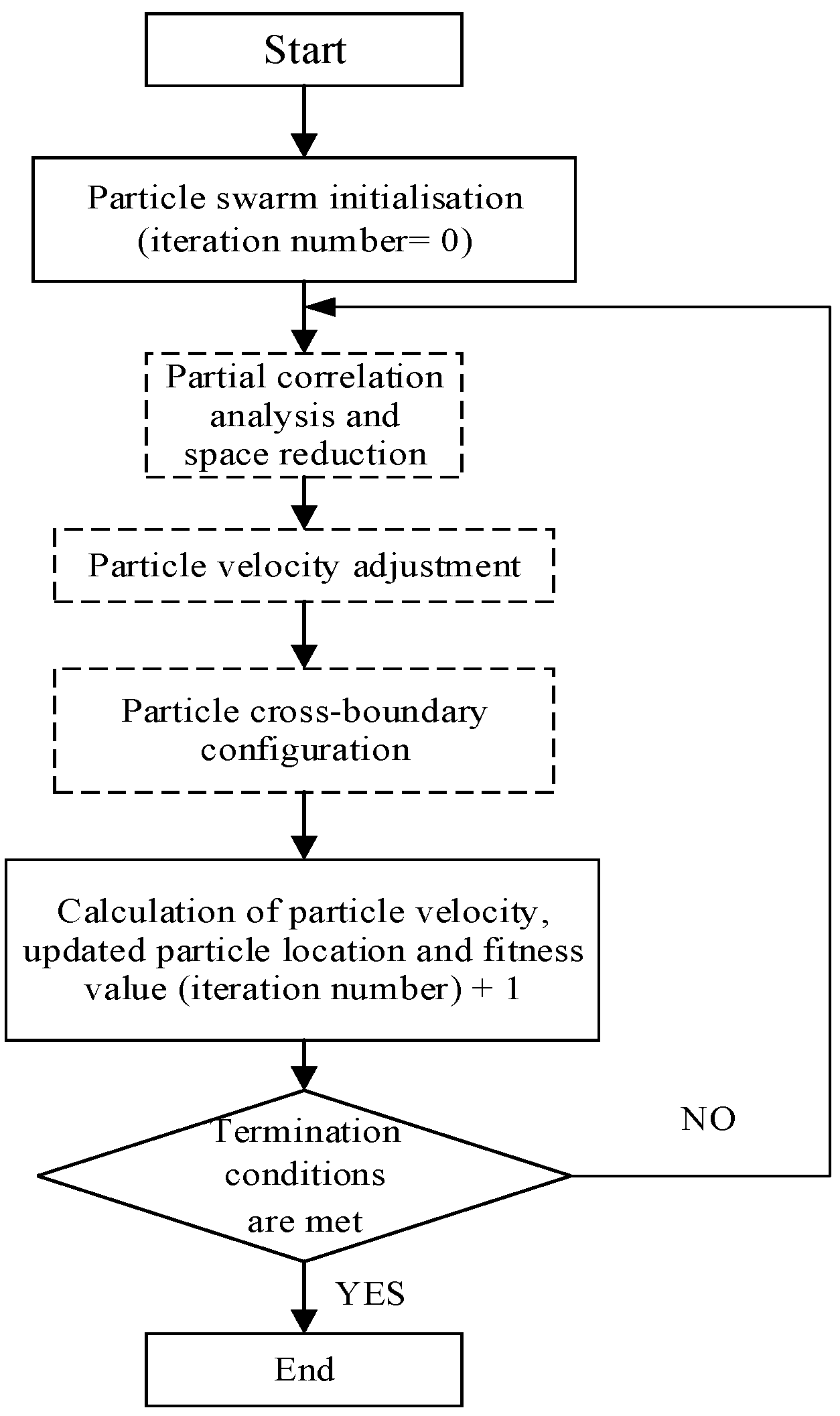
3.3. Optimisation Framework of Improved Particle Swarm Optimisation Algorithm

The flowchart of the improved PSO algorithm is shown in Figure 6. The dashed box indicates improvement measures. The specific steps are as follows:

(1)

input the parameters such as the number of particles and the number of iterations at the start of the algorithm;

(2)

perform the initialisation process by randomised sampling using the particle swarm algorithm;

(3)

perform data mining on the initialisation data and perform space reduction while completing the particle velocity adjustment;

(4)

configure the cross-boundary particles in the iterative optimisation process, and perform data mining and space reduction after reaching a certain number of iterations;

(5)

determine whether the optimisation is terminated by the maximum number of iterations.

The above improvement measures could improve the global and local optimisation ability of the PSO algorithm, which stays away from the local optimal solution and can quickly locate the optimisation space worthy of attention and improve the optimisation performance.

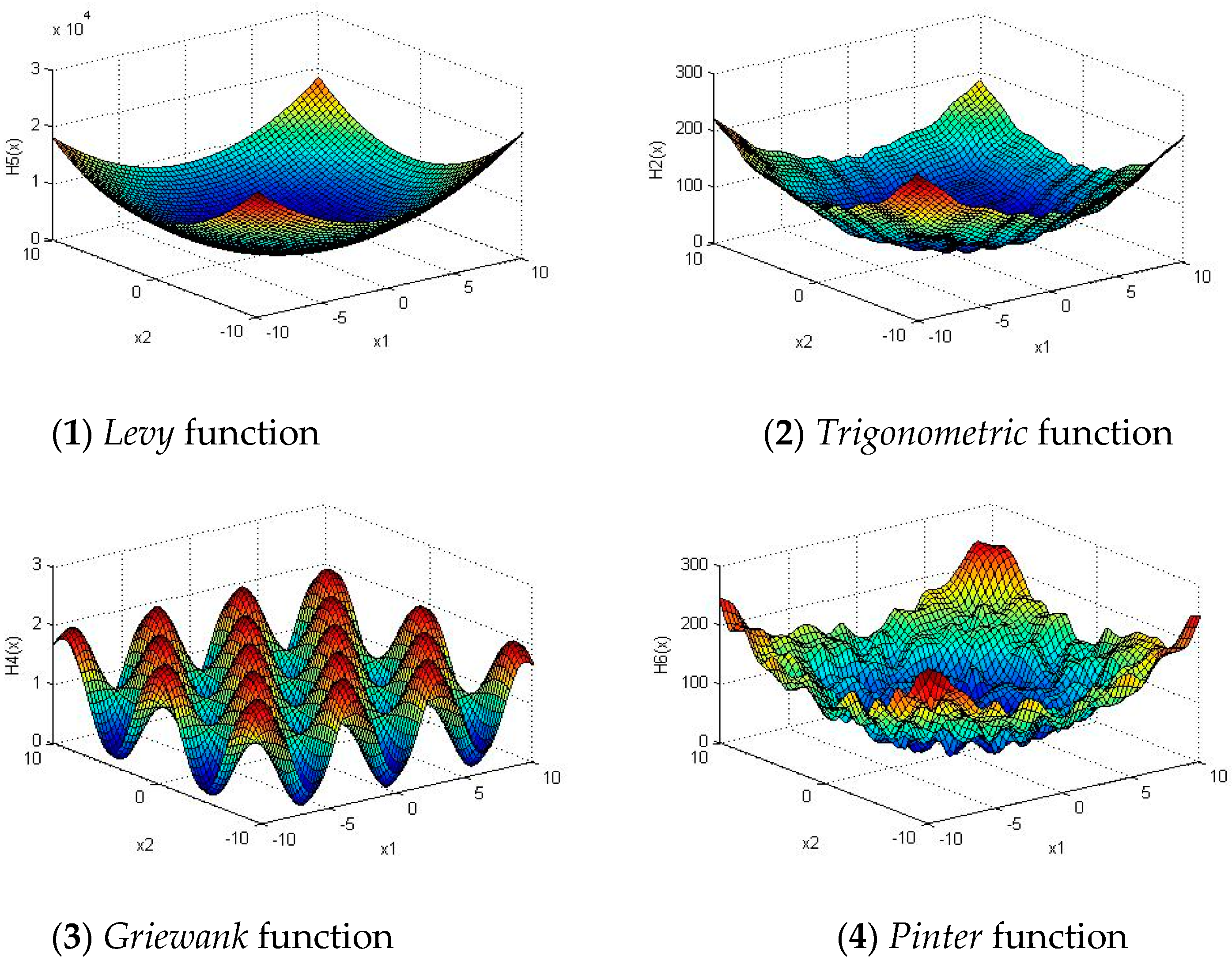
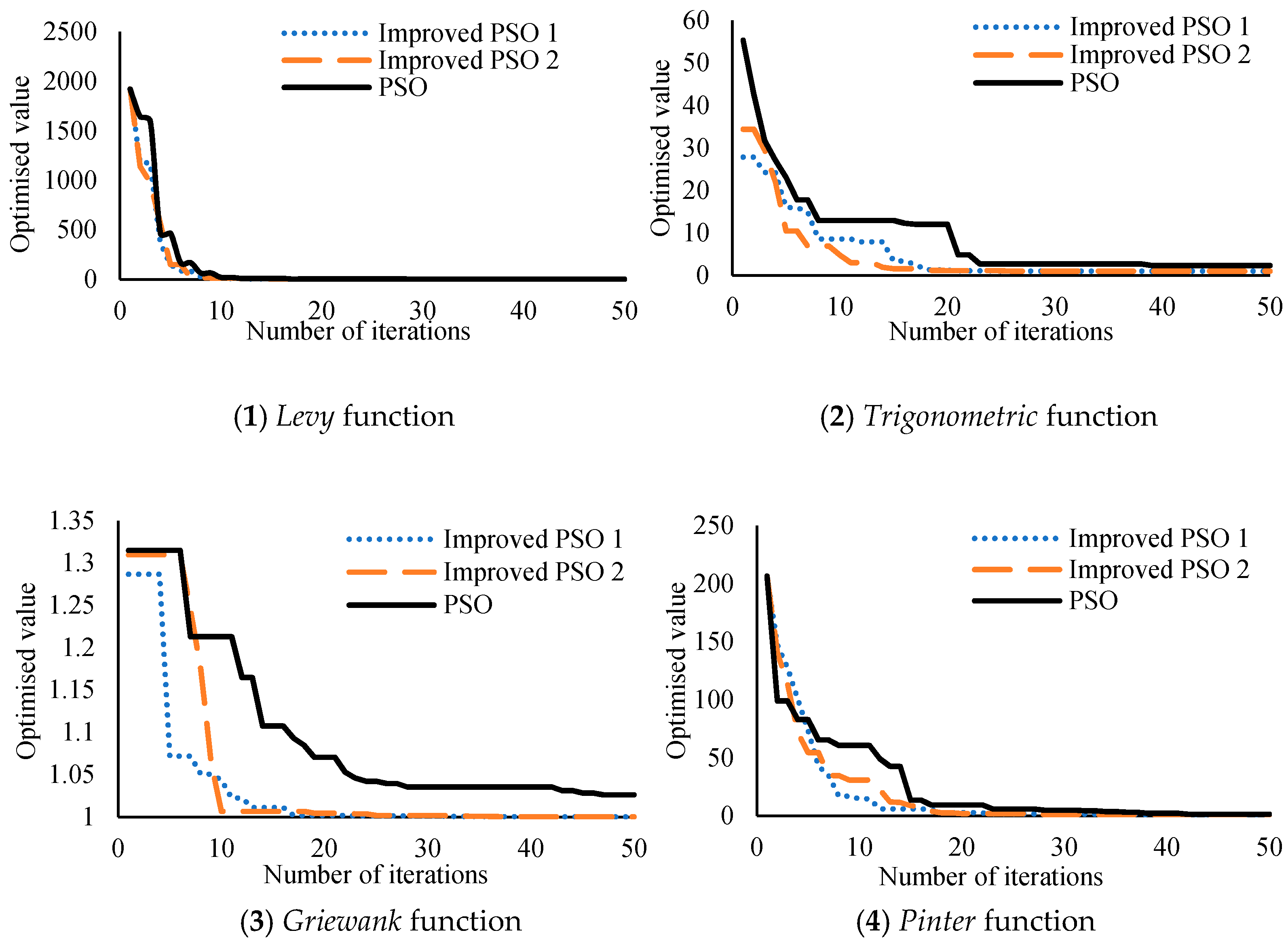
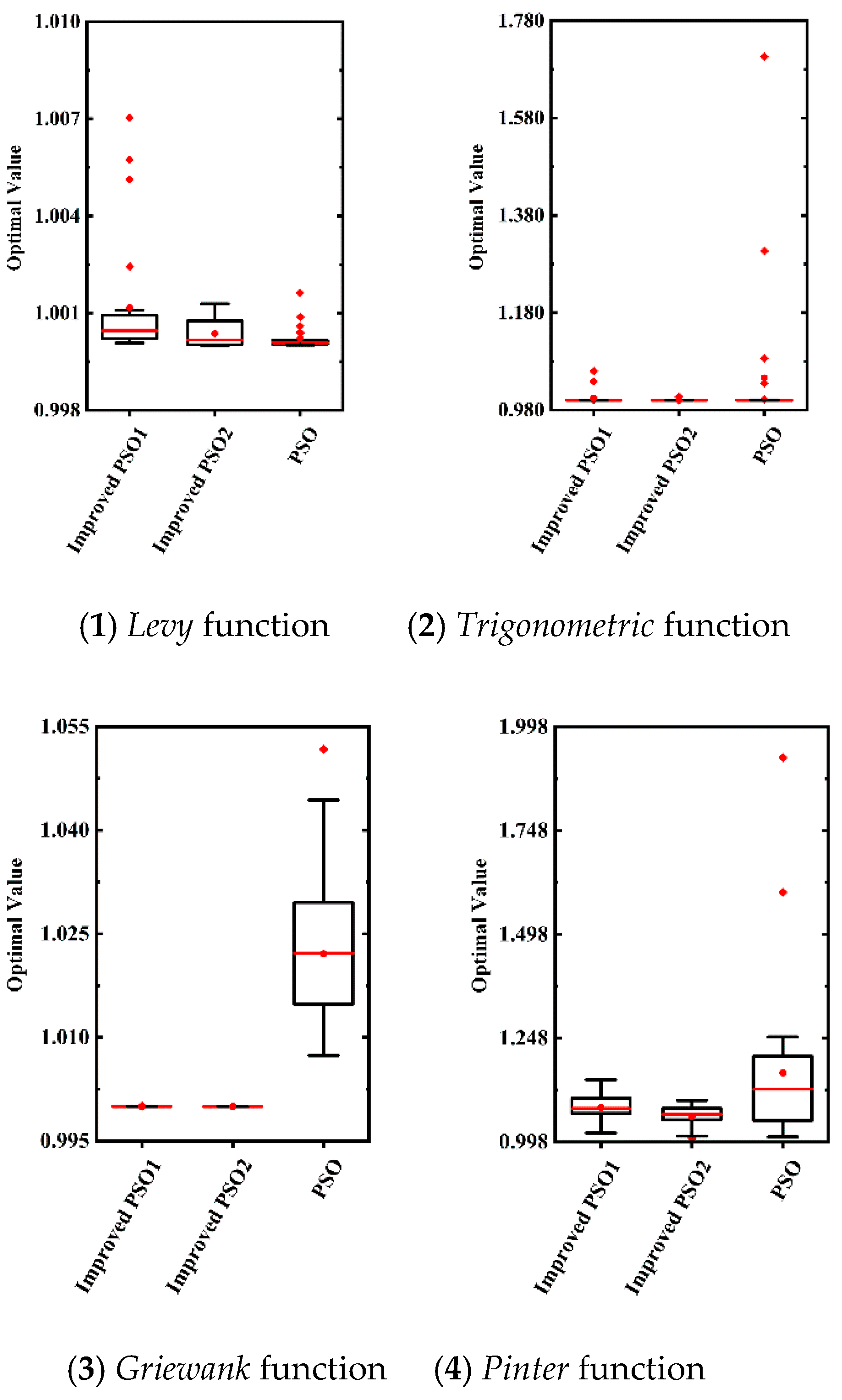
4. Function Examples of the Improved Particle Swarm Optimisation Algorithm

Four commonly used numerical functions were selected to test the performance of the algorithm. To facilitate the drafting of the optimised iteration convergence graph, the numerical results of the four selected numerical functions were all added by 1 based on the corresponding reference numerical functions. The expressions of the four numerical functions are shown in Equations (13)–(16), and the function name, test dimension, variable range, theoretical optimal scheme, and corresponding optimal solution are also given.

(1) Levy function $(n=5,-10\le x_i\le 10,i=1,\cdots ,n)$

$$H_1(x)=10 {\sin }^2(\pi x_1)+{\displaystyle \sum _{i=1}^{n-1}100 xi(1+10 {\sin }^2(\pi x_{i+1}))}+100 {(x_n-2)}^2+1$$

(13)

where $x^{*}={(0,\cdots ,0,1)}^{\mathrm{T}}$, $H_1(x^{*})=1$.

(2) Trigonometric function $(n=5,-10\le x_i\le 10,i=1,\cdots ,n)$

$$H_2(x)={\displaystyle \sum _{i=1}^n[8{\sin }^2(7{(x_i-0.9)}^2)}+6{\sin }^2(14{(x_i-0.9)}^2)+{(x_i-0.9)}^2]+1$$

(14)

where $x^{*}={(0.9,\cdots ,0.9)}^{\mathrm{T}}$, $H_2(x^{*})=1$.

(3) Griewank function $(n=5,-10\le x_i\le 10,i=1,\cdots ,n)$

$$H_3(x)=\frac{1}{4000}{\displaystyle \sum _{i=1}^n{x}_i^2}-{\displaystyle \prod _{i=1}^n\cos (\frac{x_i}{\sqrt{i}})}+2$$

(15)

where $x^{*}={(0,\cdots ,0)}^{\mathrm{T}}$, $H_3(x^{*})=1$.

(4) Pinter function $(n=5,-10\le x_i\le 10,i=1,\cdots ,n)$

$$H_4(x)={\displaystyle \sum _{i=1}^{n}i{x}_i^2}+{\displaystyle \sum _{i=1}^{n}20 i{\sin }^2}(x_{i-1}\sin x_i-x_i+\sin x_{i+1})+{\displaystyle \sum _{i=1}^{n}i{\log }_{10}}(1+i{(x_{i-1}^2-2x_i+3x_{i+1}-\cos x_i+1)}^2)+1$$

(16)

where x₀ = x_n, x_n+1 = x₁, $x^{*}={(0,\cdots ,0)}^{\mathrm{T}}$, $H_4(x^{*})=1$.

Figure 7 is a schematic diagram showing the spatial structure of the two-dimensional performance of each function.

In the function examples, both the PSO algorithm and improved PSO algorithm were applied for optimisation, and the optimised particle number was set to 100. The number of iterations was 50 generations. The space reduction methods used in the improved PSO algorithm were the segmentation reduction method and the linear reduction method mentioned in Section 3.2.2, respectively. Because the initial range of function variables was large, space reduction was set to be conducted every other generation. The optimisation iteration convergence graphs of the four functions are shown in Figure 6, and the optimisation results are shown in

Table 3. Optimised results of function algorithms.

Function Name	Optimisation Method	Convergent Algebra	Optimisation Optimal Value	Theoretical Optimal Value
Levy	PSO	12	1.296	1
	Improved PSO 1	11	1.250
	Improved PSO 2	11	1.001
Trigonometric	PSO	39	2.332	1
	Improved PSO 1	21	1.000
	Improved PSO 2	20	1.000
Griewank	PSO	28	1.026	1
	Improved PSO 1	16	1.000
	Improved PSO 2	10	1.000
Pinter	PSO	35	1.423	1
	Improved PSO 1	18	1.050
	Improved PSO 2	19	1.011

. Convergent algebra denotes the rate of convergence. In this paper, the algebra is used as a convergence standard. In Figure 8, the x-axis is the number of iterations, and the y-axis is the optimal value of the current iteration. The different line types represent different optimisation algorithms (where improved PSO algorithm 1 is the segmentation reduction method, and improved PSO algorithm 2 is the linear reduction method).

As seen in Figure 8 and Table 3, for the Levy function with a simple space, both the improved PSO algorithm and the PSO algorithm can find the optimal solution in a short time; thus, the space reduction method did not significantly improve the efficiency. For the Griewank function with a complex space, there are many local optimal solutions in the function, making the PSO algorithm fall into local optima, whereas the improved PSO algorithm can obtain the optimal solution. For the trigonometric function and the Pinter function, the improved PSO algorithm can improve the overall efficiency and performance of the optimisation. According to the specific optimisation results listed in Table 3, all optimal values obtained by the improved PSO algorithm were better than those of the PSO algorithm and were closer to the theoretical optimal value.

To demonstrate the robustness of algorithm, each function was optimized using both the improved PSO algorithm and PSO algorithm 100 times.

The obtained global optimum for each run is illustrated in Figure 9 using boxplots. A smaller or shorter box implies that the standard deviation was small, and the symbol (red points) denotes the abnormal value. The relatively smaller boxes of DSROF for most test functions validate that its robustness was higher than that of PSO, particularly in the case of complex functions. For the Levy function, both the improved PSO algorithm and the PSO algorithm can find the optimal solution. However, the standard deviation and average of the improved PSO are only a little bigger than PSO.

5. Bow Shape Optimisation in Engineering Vessel

According to the research described in Section 3, the linear function was used to establish the relationship between the partial correlation coefficient and the degree of space reduction. In this study, an engineering vessel was used to optimise the bow shape to reduce the wave-making resistance. A scale ratio of 1:20 was used to model the hull form. The main parameters of the model are shown in

Table 4. Major parameters of an engineering vessel.

Length between Perpendiculars Lpp (m)	Waterline Width Bwl (m)	Draft T (m)	Block Coefficient Cb	Drainage Volume $\nabla$ (m3)	Wet Surface Area Swet (m2)	Floating Centre Longitudinal Position Lcb (m)
4.995	0.770	0.255	0.674	0.646	4.764	2.518 m

. The front of the model has an invisible bulbous bow. The model is shown in Figure 10.

5.1. Definition of Optimisation

Optimisation Problem Definition

Three changeable control points were selected as the optimisation variables at the bow waterline position and the bilge position of the hull, which were numbered X₁–X₆. The distribution of these data in the hull is shown in Figure 11. The change direction of all optimisation variables was in the ship width (y) direction. The range of variables and initial values are shown in

Table 5. Range of the optimisation variables.

Optimisation Variable	Lower Limit	Upper Limit
Y1	0.01000	0.01300
Y2	0.04000	0.06000
Y3	0.07200	0.09700
Y4	0.08500	0.12500
Y5	0.20000	0.24000
Y6	0.17000	0.22000

.

The optimisation target is the wave-making resistance coefficient min C_w of the ship. The Froude number during ship optimisation was F_n = 0.24. The optimisation considered only the conditions of full restrictions, regardless of heave and pitch motions. To ensure that the performance of the ship does not change too much under certain drainage conditions, the drainage volume ($\mathrm{\Delta }$), and the longitudinal position of the floating centre ($L_{cb}$) were selected as the hydrostatic constraints. The specific settings are as follows.

$$\begin{gathered} 0\%\le \frac{{\Delta }_{\mathrm{opt}}-{\Delta }_{\mathrm{initial}}}{{\Delta }_{\mathrm{initial}}}\le 1\% \\ \left|\frac{L_{cb\mathrm{opt}}-L_{cb\mathrm{initial}}}{L_{cb\mathrm{initial}}}\right|\le 1\% \end{gathered}$$

Because only the bow form was optimised, and the layout was at the middle section of the ship, the tail form and the contour of the hull were constrained to keep the shape of the rear hull and the hull profile stable during the optimisation process. The hull constraint points are arranged as shown by the red line in Figure 12.

The improved PSO algorithm and the PSO algorithm were applied to the engineering vessel for optimisation. The population data generated by the initialisation were consistent. Because there are many constraints in hull form optimisation, several infeasible solutions can be generate. This makes it more complex than the function examples. Moreover, the optimisation space value of the hull variable is small. To ensure the accuracy of datamining, the partial correlation analysis must be performed every four generations, along with space reduction.

5.2. Flowchart of Hull Form Optimisation

Figure 13 is a flowchart of hull form optimisation. In our study, we used the hull surface modification method based on radial basis function interpolation [9,42,43] to obtain the new hull form. The commercial software Shipflow was used to calculate the ship wave-making resistance performance. The entire optimisation process and calculations were performed on a self-developed multi-disciplinary integrated optimisation platform for ship hydrodynamic performance [44]. The number of particles was set to 60, and the optimisation iteration was set to 20 generations. The computer used for the calculation was a 2.9-GHz Intel i9-7920x with 32 GB of RAM, running the Windows 7 operating system.

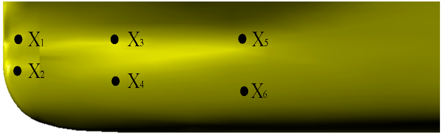
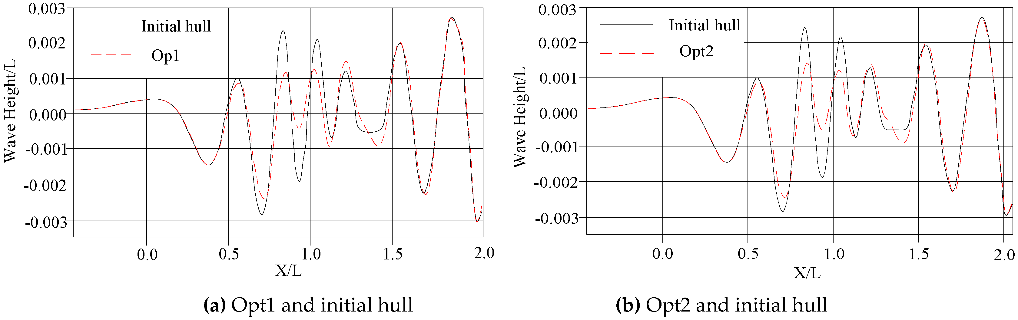
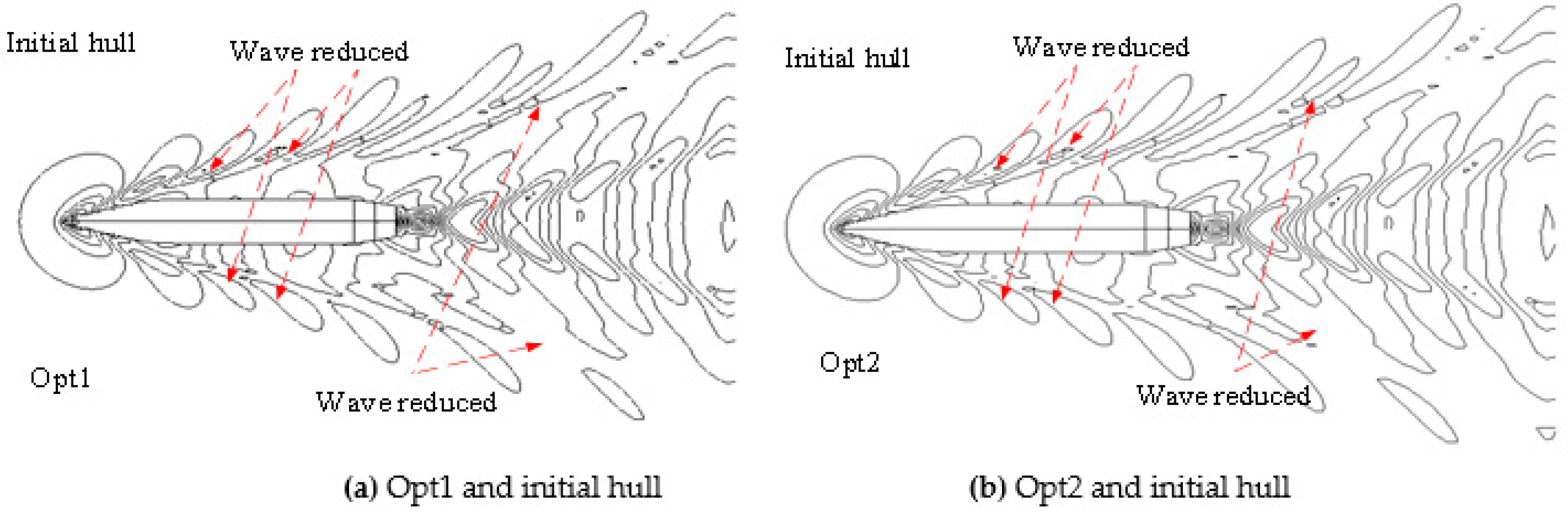
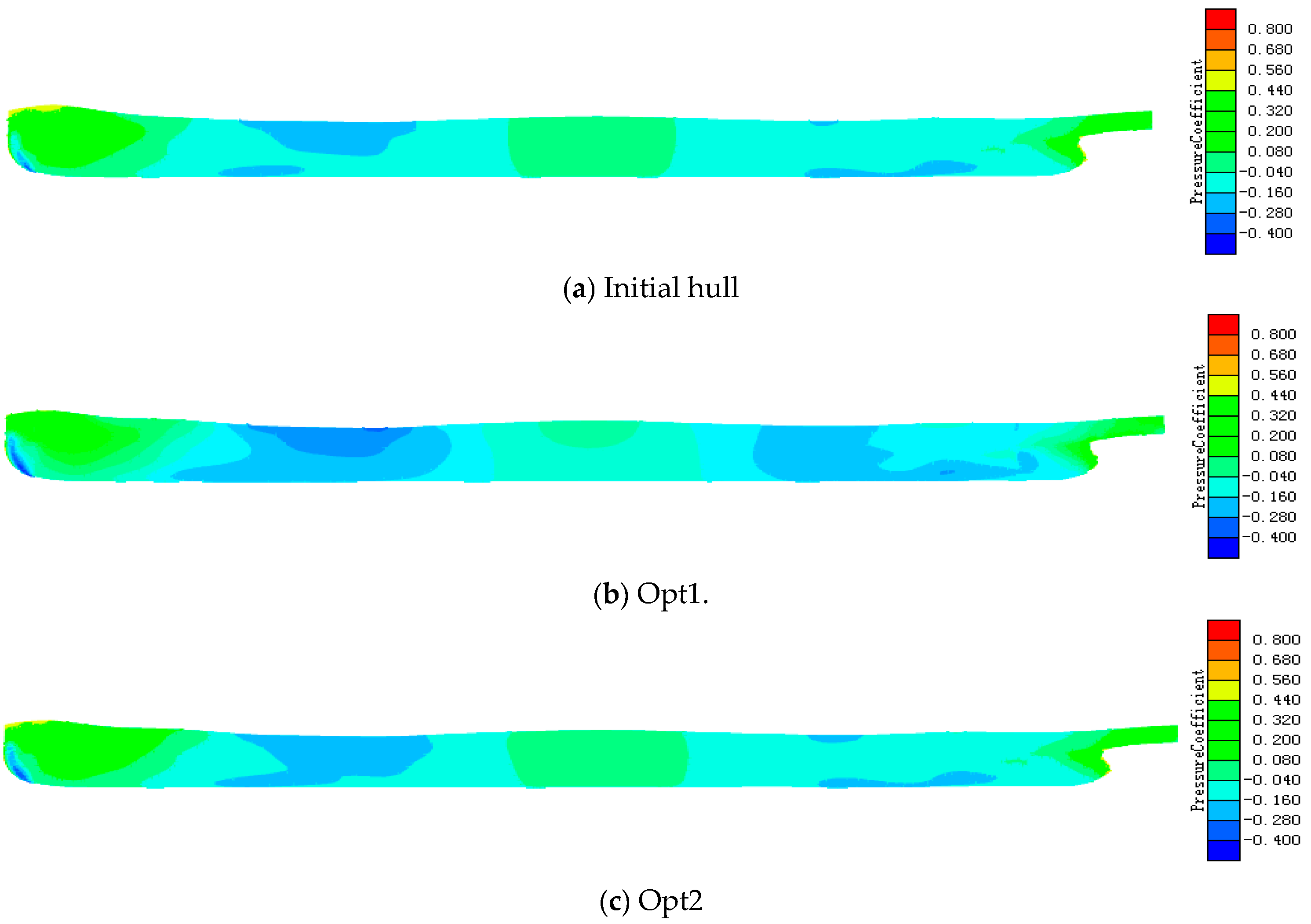
5.3. Hull Form Optimisation Results

The optimised iterative convergence graph is shown in Figure 14. The comparison shows that the improved PSO algorithm tended to converge after 11 generations, whereas the PSO algorithm tended to converge after the 17th generation. The time for the two algorithms to reach the maximum number of iterations was approximately 20 h. The time for the improved PSO algorithm to reach convergence was 11 h 30 min. The time for the PSO algorithm to reach convergence was 16 h. Therefore, the improved PSO algorithm can improve the optimisation efficiency in the example of hull form optimisation.

Table 6. Comparison of optimisation results.

Parameter	X1	X2	X3	X4	X5	X6	Cw$\times$ 103	Change
Initial hull	0.0116	0.0474	0.0859	0.1013	0.1938	0.2183	1.337	0%
Opt1	0.0107	0.0600	0.0720	0.0959	0.1941	0.2127	1.200	−10.24%
Opt2	0.0112	0.0600	0.0722	0.0939	0.1939	0.2157	1.202	−10.10%

lists the variable data comparison between the PSO algorithm (Opt1) and the improved PSO algorithm (Opt2). It shows that the optimised hull form obtained by both algorithms was basically the same. The optimised wave-making resistance coefficients were also similar. The wave-making resistance coefficient of Opt1 was reduced by 10.24%, and the wave-making resistance coefficient of Opt2 was reduced by 10.10%. These results indicated that the improved PSO algorithm can ensure satisfactory performance in the optimisation process.

Table 7. Comparison of optimisation results at Fn = 0.24.

	Floating Centre Longitudinal Position (m)	Drainage Volume (m3)	Wet Surface Area (m2)	Total Drag Coefficient Ct $\times$ 103	Change
Initial hull	2.518	0.646	4.764	4.909	0
Opt1	2.520	0.646	4.774	4.758	−3.07%
Opt2	2.519	0.646	4.773	4.764	−2.96%

lists the changes in the major parameters of the optimised hull and the initial hull using the two optimisation algorithms at Fn = 0.24. The comparison shows that the drainage volume and the longitudinal position of the floating centre of Opt1 and Opt2 were essentially the same as those of the initial hull. The wet surface area was slightly increased compared with the initial hull. The total drag coefficient of Opt1 decreased by 3.07%, and the total drag coefficient of Opt2 decreased by 2.96%. Considering the errors in CFD calculations, the hull form results obtained by the two optimisation algorithms were basically the same. The total drag coefficient was calculated by Shipflow.

The comparison between Table 6 and Table 7 shows that the hull form obtained by both the standard and improved PSO algorithms was consistent. Opt1, Opt2, and the initial hull were subjected to profile analyses. Figure 15 and Figure 16 provide a comparison of the cross-sectional line and the vertical line of the initial hull and the optimised hull. A comparison of the cross-sectional lines shows that the contour of the two optimised hulls close to the invisible bullnose was slightly increased compared with the initial hull, making the bow profile smooth, reducing the ridge vortex, and thus reducing the drag. The waterline from the bow to the middle section was slightly contracted compared with the initial hull. The bow waterline was more pointed and thinner, which reduces the inflow angle and is beneficial to reduce the wave-making resistance of the hull.

Figure 17 and Figure 18 provide a comparison of the wave profile along the hull and waveform plots of Opt1, Opt2, and the initial hull. The amplitude of the optimised hull was lower than that of the prototype hull, and the amplitude around the hull was significantly lower. The wave system of the optimised hull has become simpler, leading to a decline in the wave-making resistance. Figure 19 shows the hull pressure distribution before and after optimisation. A comparison with the prototype shows that the optimised profile reduces the positive and negative pressures at the bow and tail of the hull, thereby reducing the drag.

6. Conclusions

The PSO algorithm has the problems of local premature convergence and low convergence performance. Our study combined the space reduction techniques and improved the algorithm from different aspects, including data processing of particle swarm population initialisation, data processing of iterative optimisation, particle velocity adjustment, and particle cross-boundary configuration. Commonly used function examples were optimised to verify the feasibility of the improved PSO algorithm. Finally, our algorithm was applied to the hull form optimisation of an engineering vessel, and the optimisation result was compared with that of the PSO algorithm. The following conclusions can be drawn from our study:

(1)

For the optimisation of a simple space, the improved PSO algorithm did not significantly enhance the optimisation efficiency and performance compared with the PSO algorithm, and both algorithms can obtain fast convergence results. For more complex optimisation problems, PSO more easily falls into the local optimal solution, whereas the improved PSO algorithm can avoid the local optimum owing to datamining of the optimised data in the optimisation process, which can provide guidance on the optimisation of subsequent particles.

(2)

The application of the algorithm in engineering practice is verified by hull form optimisation. This algorithm can improve the optimisation efficiency to a certain extent while ensuring high performance, thus reducing the overall time of hull form optimisation. This has certain value in engineering applications.

(3)

Our study used partial correlation analysis for datamining. Because the coefficient obtained by a partial correlation analysis cannot directly perform space reduction, a certain relationship must be established. For optimisation with too many iterations, the segmentation reduction method and the linear reduction method may lose the optimal solution. In the particle initialisation stage, the particle information obtained cannot be evenly distributed in the optimisation space. As a result, the optimisation information obtained by the previous datamining is not accurate, leading to reduced optimisation efficiency. Further research is required to address these issues.

References

1. Campana, E.F.; Peri, D.; Tahara, Y.; Stern, F. Shape optimisation in ship hydrodynamics using computational fluid dynamics. Comput. Methods Appl. Mech. Eng. 2006, 196, 634–651. [Google Scholar] [CrossRef]
2. Peri, D. Design optimisation of ship hulls via CFD technologies. J. Ship Res. 2001, 45, 140–149. [Google Scholar] [CrossRef]
3. Harries, S. Systematic optimization—A key for improving ship hydrodynamics. Hansa 2005, 142, 36, 38, 40–42. [Google Scholar]
4. Kim, H.; Yang, C.; Jeong, S.; Noblesse, F. Hull form design exploration based on response surface method. In Proceedings of the Twenty-first International Offshore and Polar Engineering Conference, Maui, HI, USA, 19–24 June 2011. [Google Scholar]
5. Kim, H.; Yang, C. A new surface modification approach for CFD-based hull form optimisation. J. Hydrodyn. Ser. B 2010, 22, 520–525. [Google Scholar] [CrossRef]
6. Kim, H.; Yang, C.; Noblesse, F. Hull form optimisation for reduced resistance and improved seakeeping via practical designed-oriented CFD tools. In Proceedings of the Conference on Grand Challenges in Modeling & Simulation, Ottawa, ON, Canada, 11 July 2010; pp. 375–385. [Google Scholar]
7. Feng, B.; Hu, C.; Liu, Z.; Zhan, C.; Chang, H. Ship resistance performance optimisation design based on CAD/CFD. In Proceedings of the International Conference on Advanced Computer Control, Harbin, China, 18–20 January 2011; pp. 251–255. [Google Scholar]
8. Feng, B.; Dong, S.; Chang, H. The influence of experimental design method on design space exploration. In Proceedings of the International Conference on Fuzzy Systems and Knowledge Discovery IEEE, Zhangjiajie, China, 15–17 August 2015; pp. 1681–1687. [Google Scholar]
9. Shen, T.; Feng, B.; Liu, Z.; Chang, H. Research of hull form modification method based on interpolation of radial basis function. Shipbuild. China 2013, 4, 45–54. [Google Scholar]
10. Chang, H.; Cheng, X.; Liu, Z.; Feng, B.; Zhan, C. Sample selection method for ship resistance performance optimisation based on approximated model. J. Ship Res. 2016, 60, 1–13. [Google Scholar] [CrossRef]
11. Chang, H.; Feng, B.; Liu, Z.; Zhan, C.; Cheng, X. The application of approximate model for ship resistance performance optimisation. Shipbuild. China 2012, 1, 88–98. [Google Scholar]
12. Chang, H.; Feng, B.; Liu, Z.; Zhan, C.; Cheng, X. Research on application of approximate model in hull form optimisation. Shipbuild. China 2012, 53, 88–98. [Google Scholar]
13. Harries, S.; Abt, C. Faster turn-around times for the design and Optimization of functional surfaces. Ocean Eng. 2019, 193, 106470.1–106470.18. [Google Scholar] [CrossRef]
14. D’Agostino, D.; Serani, A.; Diez, M. Design-space assessment and dimensionality reduction: An off-line method for shape reparameterization in simulation-based Optimization. Ocean Eng. 2020, 197, 106852. [Google Scholar] [CrossRef]
15. Serani, A.; Stern, F.; Campana, E.F.; Diez, M. Hull-form stochastic Optimization via computational-cost reduction methods. Eng. Comput. 2021, 2, 1–25. [Google Scholar]
16. Khan, S.; Serani, A.; Diez, M.; Kaklis, P. Physics-Informed Feature-to-Feature Learning for Design-Space Dimensionality Reduction in Shape Optimization. In Proceedings of the AIAA Scitech 2021 Forum, Music City Center Nashville, Nashville, TN, USA, 11–15 & 19–21 January 2021. [Google Scholar]
17. Tezzele, M.; Salmoiraghi, F.; Mola, A.; Rozza, G. Dimension reduction in heterogeneous parametric spaces with application to naval engineering shape design problems. Adv. Modeling Simul. Eng. Sci. 2018, 5, 1–19. [Google Scholar] [CrossRef] [Green Version]
18. Serani, A.; Pellegrini, R.; Wackers, J.; Jeanson, C.E.; Diez, M. Adaptive multi-fidelity sampling for CFD-based Optimization via radial basis function metamodels. Int. J. Comput. Fluid Dyn. 2019, 33, 237–255. [Google Scholar] [CrossRef]
19. Chunna, L.; Hai, F.; Chunlin, G. Development of an efficient global Optimization method based on adaptive infilling for structure Optimization. Struct. Multidiplinary Optim. 2020, 7, 3383. [Google Scholar]
20. Zhang, S.; Zhang, B.; Tezdogan, T.; Xu, L.; Lai, Y. Computational fluid dynamics-based hull form Optimization using approximation method. Eng. Appl. Comput. Fluid Mech. 2018, 12, 74–88. [Google Scholar] [CrossRef] [Green Version]
21. Coppedè, A.; Gaggero, S.; Vernengo, G.; Villa, D. Hydrodynamic shape Optimization by high fidelity CFD solver and Gaussian process based response surface method. Appl. Ocean Res. 2019, 90, 101841. [Google Scholar] [CrossRef]
22. Pellegrini, R.; Serani, A.; Liuzzi, G.; Rinaldi, F.; Diez, M. Hybridization of Multi-Objective Deterministic Particle Swarm with Derivative-Free Local Searches. Mathematics 2020, 8, 546. [Google Scholar] [CrossRef] [Green Version]
23. Tezdogan, T.; Zhang, S.; Demirel, Y.K.; Liu, W.; Xu, L.; Yuyan, L. An investigation into fishing boat optimisation using a hybrid algorithm. Ocean Eng. 2018, 167, 204–220. [Google Scholar] [CrossRef] [Green Version]
24. Serani, A.; Leotardi, C.; Iemma, U.; Campana, E.F.; Fasano, G.; Diez, M. Parameter selection in synchronous and asynchronous deterministic particle swarm optimization for ship hydrodynamics problems. Appl. Soft Comput. 2016, 49, 313–334. [Google Scholar] [CrossRef] [Green Version]
25. Leotardi, C.; Serani, A.; Diez, M.; Campana, E.F.; Gusso, R. Dense conjugate initialization for deterministic PSO in applications: ORTHOinit+. Appl. Soft Comput. 2021, 4, 107121. [Google Scholar] [CrossRef]
26. Khalili-Damghani, K.; Abtahi, A.R.; Tavana, M. A new multi-objective particle swarm optimisation method for solving reliability redundancy allocation problems. Reliab. Eng. Syst. Saf. 2013, 111, 58–75. [Google Scholar] [CrossRef]
27. Kennedy, J.; Eberhart, R.C.; Shi, Y. The Particle Swarm. Swarm Intell. 2001, 1, 287–325. [Google Scholar]
28. Angeline, P.J. Evolutionary optimization versus particle swarm optimization: Philosophy and performance differences. In Proceedings of the 7th Annual Conference on Evolutionary Programming, San Diego, CA, USA, 25–27 March 1998. [Google Scholar]
29. Eberhart, R.C.; Shi, Y. Comparison between Genetic Algorithms and Particle Swarm Optimization; Springer: Berlin/Heidelberg, Germany, 1998. [Google Scholar]
30. Cheng, S.; Shi, Y.; Qin, Q. Dynamical exploitation space reduction in particle swarm optimisation for solving large scale problems. In Proceedings of the Evolutionary Computation, IEEE, Brisbane, QLD, Australia, 10–15 June 2012; pp. 1–8. [Google Scholar]
31. Noel, M.M. A new gradient-based particle swarm optimisation algorithm for accurate computation of global minimum. Appl. Soft Comput. J. 2012, 12, 353–359. [Google Scholar] [CrossRef]
32. Shi, J.; Li, P.; Liu, G.; Liu, P. Parameter Estimation of Chaotic Systems Based on Improved Particle Swarm Optimisation Algorithm. J. Huazhong Univ. Sci. Technol. 2018, 46, 70–76. [Google Scholar]
33. Reungsinkonkarn, A.; Apirukvorapinit, P. Search space reduction of particle swarm optimisation for hierarchical similarity measurement model. In Proceedings of the Computer Science and Software Engineering (JCSSE), 2014 11th International Joint Conference, Chon Buri, Thailand, 14–16 May 2014. [Google Scholar]
34. Zhang, L.; Sun, J.; Guo, C. A novel multi-objective discrete particle swarm optimisation with elitist perturbation for reconfiguration of ship power system. Pol. Marit. Res. 2017, 24, 1. [Google Scholar]
35. Wang, J.; Li, H. Particle swarm optimisation with enhanced global search and local search. J. Intell. Syst. 2017, 26, 3. [Google Scholar]
36. Wu, K.; Feng, B.; Chang, H. The design method for hull optimisation based on partial correlation analysis. Ship Eng. 2016, 10, 46–51. [Google Scholar]
37. He, X. Modern Statistical Analysis Methods and Applications. Master’s Thesis, Renmin University Press, Beijing, China, 1998. [Google Scholar]
38. Jia, J. Statistical Case Studies and Analysis. Master’s Thesis, Renmin University Press, Beijing, China, 2010. [Google Scholar]
39. Coello, C.A.C.; Pulido, G.T.; Lechuga M, S. Handling multiple objectives with particle swarm optimisation. IEEE Trans. Evol. Comput. 2004, 8, 256–279. [Google Scholar] [CrossRef]
40. Coello, C.A.C.; Lamont, G.B.; Veldhuizen, D.A.V. Evolutionary Algorithms for Solving Multi-Objective Problems; Springer: Berlin/Heidelberg, Germany, 2002; p. 576. [Google Scholar]
41. Fang, K.T. Uniform design: An application of number-theoretic methods to experimental designs. Acta Math. Appl. Sin. 1980, 3, 363–372. [Google Scholar]
42. Cheng, X.; Shen, T.; Feng, B.; Liu, Z. The determination method and application of support radius in hull surface deformation. Shipbuild. China 2016, 57, 127–137. [Google Scholar]
43. Shen, T. The method and application of hull surface deformation based on radial basis function interpolation. Ph.D. Thesis, Wuhan University of Technology, Wuhan, China, 2015. [Google Scholar]
44. Zheng, Q. Development and application of an interdisciplinary and comprehensive optimisation platform for ship hydrodynamic performance. In Proceedings of Digital Shipbuilding Conference in 2018; The Chinese Society of Naval Architects and Marine Engineers: Shanghai, China, 2018; p. 6. [Google Scholar]
Figure 1. Function relationship plot ( x 0 , 1 ).
Jmse 09 00955 g001
Figure 2. Function relationship plot ( x 1 , 1 ).
Jmse 09 00955 g002
Figure 3. Function relationship plot.
Jmse 09 00955 g003
Figure 4. Examples of random sampling.
Jmse 09 00955 g004
Figure 5. Examples of uniform design sampling.
Jmse 09 00955 g005
Figure 6. Flowchart of improved particle swarm optimisation algorithm.
Jmse 09 00955 g006
Figure 7. Schematic diagram showing the spatial structure of the two-dimensional performance of each function.
Jmse 09 00955 g007
Figure 8. Optimised iterative convergence plot.
Jmse 09 00955 g008
Figure 9. Boxplot of the best solution for all test problems.
Jmse 09 00955 g009
Figure 10. Hull model.
Jmse 09 00955 g010
Figure 11. Distribution of the optimisation variables.
Jmse 09 00955 g011
Figure 12. Arrangement of hull constraint points.
Jmse 09 00955 g012
Figure 13. Flowchart of hull form optimisation with dynamic space reduction.
Jmse 09 00955 g013
Figure 14. Optimised iterative convergence graph.
Jmse 09 00955 g014
Figure 15. Cross-sectional line comparison chart.
Jmse 09 00955 g015
Figure 16. Vertical line comparison chart.
Jmse 09 00955 g016
Figure 17. Wave profile along the hull at Fn = 0.24 (y/L = −0.301).
Jmse 09 00955 g017
Figure 18. Fn = 0.24 waveform.
Jmse 09 00955 g018
Figure 19. Fn = 0.24 hull pressure distribution map.
Jmse 09 00955 g019