Application of Basis Functions for Hull Form Surface Modification

Abstract

Basis functions are key in constructing interpolation equations in hull surface modification based on radial basis functions (RBF) interpolation. However, few have studied the selection of basis functions in depth. By comparing several typical basis functions through a theoretical analysis and two-dimensional modification examples, the Wendland ψ3,1 (W) function is selected. The advantages of hull form surface modification based on W function interpolation are further validated through a case study. Finally, the modification method is used to optimize a trimaran model. An optimal hull form with fair lines is obtained, and its wave-making resistance coefficient and total resistance are reduced by 8.3% and 3.8%, respectively, compared to those of the original model. These findings not only further illustrate that the W function is relatively suitable for hull form surface modification, but also validate the feasibility and value of the RBF interpolation-based surface modification method in engineering practice.

1. Introduction

The International Maritime Organization proposed an energy efficiency design index (EEDI) in 2009. Optimizing the drag performance of ships is an effective way to meet EEDI requirements. With the rapid development of computer technology and computational fluid dynamics (CFD), simulation-based hull line optimization has become a central research topic. Cheng et al. [1], Abt et al. [2], Peri et al. [3,4], Campana et al. [5], Li [6], Zhao et al. [7], Yang et al. [8,9], Tahara et al. [10], Feng Baiwei [11,12] Chang Haichao [13,14], Wei [15,16], and Zheng [17] integrated computer-aided design (CAD) with CFD based on numerical simulation techniques and optimization algorithms, established CFD-based hull line optimization platforms, successfully completed optimized designs of hull lines through simulation, and obtained optimized hull forms with excellent hydrodynamic performance.

To complete the fine optimization of hull lines, Xu et al. [18] tracked the development of a classified optimization program, which consisted of five layers and illustrated that CFD codes are suitable for optimizing hull lines in order to improve drag performance. Harries et al. [19] proposed a parameterization method, constructed a model using the Friendship software, and performed hydrodynamic calculations using SHIPFLOW software. Peri et al. [20,21] studied a variable fidelity method and accelerated the optimization process for a multi-objective design problem using the free-surface Reynolds-averaged Navier–Stokes (RANS) method. Tahara et al. [22] optimized the stern and the combined bulbous bow and sonar dome of a ship based on finite difference gradients. Peri et al. [23] introduced a simulation-based design optimization technique to solve engineering optimization problems involving objective functions and nonlinear constraints that are complex and have a high computational cost. By combining the Rankine source method and nonlinear programming (NLP), Zhang et al. [24] optimized hull lines with the minimum wave-making resistance RW based on CFD. Peri [4] proposed a method that can optimize the robustness of the conceptual design of a bulk cargo ship based on uncertain operating and environmental conditions, and applied the particle swarm optimization (PSO) algorithm in the global minimization process, thereby maximally reducing the expected value and standard deviation of the per unit transportation cost. Since then, the feasibility of robust design optimization (RDO) based on actual operating ship data has been demonstrated. Grigoropoulos et al. [25] proposed an improved hull line optimization method without considering calm water resistance and its sea-keeping ability. Yang et al. [9] developed an efficient and effective hull surface modification technique for CFD-based hull line optimization in order to modify the local and overall hull lines. Guerrero et al. [26] present a shape optimization workflow entirely based on open-source tools; it is fault tolerant and software agnostic, allows for asynchronous simulations, and has a high degree of automation.

The hull surface modification method plays an important role in a hull form optimization framework. There are currently two main types of hull surface modification methods for hull form optimization. The first type modifies the surface of a certain ship area by changing the coordinates of the control vertices of the non-uniform rational basis spline (NURBS) and the basis spline (B-spline) of this area or by directly modifying the coordinates of the hull offsets based on the mathematical expressions (NURBS and B-spline) of the hull surface. The second type is composed of hull form parameter-based parameterization methods. These methods change the hull form by extracting the typical characteristic parameters for the geometric shape of the hull and changing them through functions.

Form modification methods that directly use offsets or grid control vertices as variables can generate complex hull forms. However, these methods require a large number of control points to modify a certain hull surface area, which can result in an increase in the optimization time. If there are a relatively large number of variables, these methods may be unable to ensure fair local hull lines. In light of this, researchers have developed an integration method, a Bezier patch method and a free form modification method. These methods essentially change the coordinates of the control points, but have significantly fewer optimization variables and are also able to ensure fair hull lines. The shortcoming of the integration method is that it requires a certain number of parent ships, otherwise it cannot obtain the maximum amount of hull forms by integration. The Bezier patch method is mainly applicable to local form modification. An increase in the number of design variables can result in a significant increase in the computational time. The free form modification method is applicable to the overall form modification but involves a relatively large number of design variables.

The advantages of the parametric modeling method lie in the fact that each control parameter has a definite geometric meaning and can be flexibly defined manually, and that the control parameters can be directly used as design variables for overall and local ship optimization problems. However, it has the following main shortcoming. The parametric design method constructs a geometric model of the ship in a fully constrained environment. All the information required by the hull model is defined by parameters or constraints, and the designer can only design with the already defined parameters. Each parametric model can only be used to design a certain specific problem, and a new model requires the construction of a new parametric model. Due to its limitation, parameterization cannot meet the requirements of the conceptual design of ships, thus restricting the development and application of the parameterization technique in ship design [27]. Feng et al. [12] proposed an improved fairness criterion and calculation method based on Harries’s parameterization approach, and applied them in the parametric modeling of ships.

In recent years, surface modification methods based on Radial Basis Function (RBF) interpolation have been developed. Radial basis function interpolation is an effective tool in approximation theory, and it is also a method in the interpolation of scattered data. It has the advantages of simple calculation method, less time, flexible node configuration and high precision. At present, radial basis function interpolation technology has been widely used as a tool for interpolating or approximating scattered data, and has been widely used in mesh deformation, large dataset interpolation, pattern registration, and geology. C. Groth et al. [28] applied RBF mesh deformation to structural optimization; Vaclav Skala [29] used tightly supported radial basis functions in large dataset interpolation and analyzed interpolation properties; Deng [30] combined global deformation and local deformation, based on compactly supported radial basis functions’ complete cranial registration; Haiyang et al. [31] performed terrain interpolation based on region decomposition and Schwarz parallel principle, constructed a global interpolation matrix based on all terrain sampling data with compactly supported radial basis functions, and adaptively solved the sub-region interpolation node tight support radius. Kim et al. [32,33] used the RBF interpolation method to modify hull surfaces and optimize the drag performance of the KRISO container ship (KCS) and Series 60 hull forms, obtaining high-performance hull form schemes. Fuxin Huang et al. [34] developed a hydrodynamic optimization tool based on computational fluid dynamics to generate bulbous by surface deformation based on radial basis function interpolation. Shen et al. [35] studied the application of the RBF interpolation method in hull form optimization and used a hull form optimization platform to achieve an automatic modification of the bow and stern surfaces of the KCS hull form. Buhmann [36], Biancolini [37] and other scholars have also conducted in-depth research on the theoretical and engineering applications of radial basis functions. All of the above have laid a good foundation for the research in this paper.

In the RBF interpolation method, the key to the interpolation equation lies in the selection of the basis function. The basis function determines how the equation passes through each sample point. The relevant studies focus on explaining the basic principle of the RBF interpolation technique and the process by which it is applied in hull surface modification. Based on several typical basis functions, this study focuses on thoroughly investigating the selection of the basis function from the perspectives of theory and application. By comparing several typical basis functions through a theoretical analysis and two-dimensional modification examples, the Wendland ψ3,1 (W) is effective in local contraction, compression, and distortion, and can result in a relatively gentle transition to the boundaries and preserve the geometric relations in the original graph to a relatively satisfactory level. Additionally, by adjusting the support radius, the W RBF can have the properties of both local and global basis functions within a certain range, and can thus be used flexibly. Furthermore, the W function is compactly supported and solvable, and is also advantageous in terms of computational time. Therefore, it is suitable to use the W function as a basis function to modify hull surfaces.

This article is organized as follows. Section 1 introduces the basic theory of the RBF-based hull surface interpolation method and the establishment of a surface modification interpolation equation. Section 2 introduces several typical basis functions. Section 3 presents the application of typical basis functions in two-dimensional (2D) surface and grid point modification problems. Section 4 presents the application of the Wendland ψ3,1 (W) RBF interpolation-based surface modification method in hull surface modification. Section 5 presents the application of the W RBF interpolation-based surface modification method in hull form optimization and analyzes the optimization results. Section 6 summarizes this study, and provides an outlook for future research.

2. RBF-Based Hull Surface Interpolation

The RBF interpolation method is a precise interpolation method. The surface generated by the RBF interpolation method passes through each known sample point.

2.1. Basic Theory

An RBF uses the Euclidean distance $‖x-x_i‖$ between an arbitrary point x_i and a certain center x in the space as an independent variable. Each RBF has the following form:

$$\varphi (‖x-x_i‖)i=1,2,\dots ,n$$

(1)

A multi-variable interpolation problem is fundamentally described as a problem of making a given set of discrete data $\left\{x_i,f_i\right\},i=1,2,\dots ,n$ meet the following interpolation conditions:

$$S(x_i)=f_i i=1,2,\dots ,n$$

(2)

This problem can be solved using the RBF interpolation equation in the following form.

$$S(x)={\displaystyle \sum _{i=1}^n{\lambda }_i}\varphi \left(‖x-x_i‖\right)$$

(3)

where the function $\varphi (‖x-x_i‖)$ is an RBF and ${\lambda }_i$ is the weight coefficient. By substituting the known sample points into Equations (2) and (3), the following system of linear equations with respect to ${\lambda }_i$ are obtained:

$$\left[\begin{array}{ccccc}{\varphi }_{11}& \cdots & {\varphi }_{1i}& \cdots & {\varphi }_{1n}\\ ⋮& ⋮& ⋮& ⋮& ⋮\\ {\varphi }_{i1}& \cdots & {\varphi }_{ii}& \cdots & {\varphi }_{in}\\ ⋮& ⋮& ⋮& ⋮& ⋮\\ {\varphi }_{n1}& \cdots & {\varphi }_{ni}& \cdots & {\varphi }_{nn}\end{array}\right]\left[\begin{array}{c}{\lambda }_1\\ ⋮\\ {\lambda }_i\\ ⋮\\ {\lambda }_n\end{array}\right]=\left[\begin{array}{c}{f}_1\\ ⋮\\ f_i\\ ⋮\\ f_n\end{array}\right]$$

(4)

where ${\varphi }_{ij}=\varphi \left(‖x_i-x_j‖\right),i,j=1,2,\dots ,n$.

Let

$$F={\left[f_1,f_2,\dots f_n\right]}^T$$

$$\lambda ={\left[{\lambda }_1,{\lambda }_2,\dots {\lambda }_n\right]}^T$$

$$A=\left[\begin{array}{ccccc}{\varphi }_{11}& \cdots & {\varphi }_{1i}& \cdots & {\varphi }_{1n}\\ ⋮& ⋮& ⋮& ⋮& ⋮\\ {\varphi }_{i1}& \cdots & {\varphi }_{ii}& \cdots & {\varphi }_{in}\\ ⋮& ⋮& ⋮& ⋮& ⋮\\ {\varphi }_{n1}& \cdots & {\varphi }_{ni}& \cdots & {\varphi }_{nn}\end{array}\right]$$

Thus, the above equation can be simplified as follows:

$$A\lambda =F$$

(5)

If A is nonsingular, then Equation (5) can be simplified as follows:

$$\lambda =A^{-1}F$$

(6)

or an arbitrary data point set $\{x_i,f_i\}\in R^d\otimes R\left(i=1,\cdots ,n\right)$, the necessary and sufficient condition for the above interpolation problem to have a unique solution is that for any two different $\left\{x_i\right\}$, the symmetric matrix A is definitely positive when $x_i,i=1,\cdots ,n$ are different from one another.

2.2. Construction of a Surface Modification Interpolation Equation

When this interpolation method is used to modify a hull surface, the following form is used in the interpolation equation:

$$S(X)={\displaystyle \sum _{i=1}^n{\lambda }_i}\varphi (‖X-X_i‖)+p(X)$$

(7)

It can be proven that Equation (7) is an interpolation equation. In Equation (7), $S(X)$ is the displacement of a certain control point X = (x, y, z) on the hull surface; n is the number of control points; $‖X-X_i‖$ is the Euclidean distance between any arbitrary point X_i and the control point X; $\varphi$ is the selected RBF; and $p\left(X\right)$ is a low-order polynomial of the following form:

$$p(X)=c_{1}x+c_{2}y+c_{3}z+c_4$$

(8)

The degree of wrinkling of the surface reflects the amount of energy of the surface. To make the surface as smooth as possible, the surface energy should be as low as possible.

Equation (7) can minimize the energy of the surface [38], that is, the smoothness of the surface is guaranteed. Additionally, it can be determined that the interpolation equation consists of two parts. The first part, which consists of a linear superposition of an n number of radial interactions, characterizes the essential difference in the shape between the original point set and the modification target point set. The second part is a linear polynomial, which ensures surface continuity and corresponds to affine transformations between the two point sets, including rotation and translation. The following shows the second part in detail:

$$\left[\begin{array}{c}{x}^{,}\\ y^{,}\\ z^{,}\end{array}\right]=\left[\begin{array}{ccc}{c}_{1x}& c_{2x}& c_{3x}\\ c_{1y}& c_{2y}& c_{3y}\\ c_{1z}& c_{2z}& c_{3z}\end{array}\right]\cdot \left[\begin{array}{c}x\\ y\\ z\end{array}\right]+\left[\begin{array}{c}{c}_{4x}\\ c_{4y}\\ c_{4z}\end{array}\right]=A\cdot \left[\begin{array}{c}x\\ y\\ z\end{array}\right]+T$$

(9)

In the geometric transformation, A represents a composite transformation involving rotation, scaling, and shear transformation, and T represents the translation variable. The interpolation equation in this form accurately describes the modification of the original point set to the modified target point set.

The coefficients ${\lambda }_i$ and $c_i$ in the equation are obtained by changing the coordinates of the control points:

$$S(X_i)=f_i,i=1,2,\dots ,n$$

(10)

where $f_i$ represents the change in the coordinates of the control points. The changes in the coordinates before and after the movement of n control points are substituted into the above equation. After adding a polynomial $p\left(x\right)$ to ensure that the equation has a solution, the orthogonal constraints of the weight coefficients are also considered:

$${\displaystyle \sum _{k=1}^n{\lambda }_{\mathrm{k}}}·x_k=0;{\displaystyle \sum _{k=1}^n{\lambda }_{\mathrm{k}}}·y_k=0;{\displaystyle \sum _{k=1}^n{\lambda }_{\mathrm{k}}}·z_k=0;{\displaystyle \sum _{k=1}^n{\lambda }_{\mathrm{k}}}=0$$

(11)

Based on the above, a matrix of the following form is obtained:

$$\left[\begin{array}{cccccccc}{\varphi }_{11}& {\varphi }_{12}& \cdots & {\varphi }_{1n}& x_1& y_1& z_1& 1\\ {\varphi }_{21}& {\varphi }_{22}& \cdots & {\varphi }_{2n}& x_2& y_2& z_2& 1\\ ⋮& ⋮& \ddots & ⋮& ⋮& ⋮& ⋮& ⋮\\ {\varphi }_{n1}& {\varphi }_{n2}& \cdots & {\varphi }_{nn}& x_n& y_n& z_n& 1\\ x_1& x_2& \cdots & x_n& 0& 0& 0& 0\\ y_1& y_2& \cdots & y_3& 0& 0& 0& 0\\ z_1& z_2& \cdots & z_n& 0& 0& 0& 0\\ 1& 1& \cdots & 1& 0& 0& 0& 0\end{array}\right]\left[\begin{array}{c}{\lambda }_1\\ {\lambda }_2\\ ⋮\\ {\lambda }_n\\ c_1\\ c_2\\ c_3\\ c_4\end{array}\right]=\left[\begin{array}{c}{f}_1\\ f_2\\ ⋮\\ f_n\\ 0\\ 0\\ 0\\ 0\end{array}\right]$$

(12)

Let

$$\lambda ={[{\lambda }_1,{\lambda }_2,\dots ,{\lambda }_n]}^T,$$

$$c={[c_1,c_2,c_3,c_4]}^T$$

$$F={[f_1,f_2,\dots ,f_n]}^T$$

$$A_{i,j}=\varphi (‖x_i-x_i‖),I,j=1,2,\dots ,n\mathrm{and}$$

$$q=\left[\begin{array}{cccc}{x}_1& y_1& z_1& 1\\ x_2& y_2& z_2& 1\\ ⋮& ⋮& ⋮& ⋮\\ x_n& y_n& z_n& 1\end{array}\right]$$

Thus, Equation (12) can be simplified as follows:

$$\left(\begin{array}{c}F\\ 0\end{array}\right)=\left(\begin{array}{cc}A& q\\ q^T& 0\end{array}\right)\left(\begin{array}{c}\lambda \\ c\end{array}\right)$$

(13)

By expanding Equation (12), an independent equation in each direction (x, y and z) is obtained:

$$f_x=S_x(X)={\displaystyle \sum _{i=1}^n{\lambda }_{ix}\varphi (‖X-X_i‖)}+c_{1x}x+c_{2x}y+c_{3x}z+c_{4x}$$

(14)

$$f_y=S_y(X)={\displaystyle \sum _{i=1}^n{\lambda }_{iy}\varphi (‖X-X_i‖)}+c_{1y}x+c_{2y}y+c_{3y}z+c_{4y}$$

(15)

$$f_z=S_z(X)={\displaystyle \sum _{i=1}^n{\lambda }_{iz}\varphi (‖X-X_i‖)}+c_{1z}x+c_{2z}y+c_{3z}z+c_{4z}$$

(16)

A matrix equation in the same form as Equation (13) can be obtained in each direction (x, y, and z). The RBF interpolation ultimately boils down to solving the system of linear equations shown in Equation (13); i.e., the inversion of a high-dimensional matrix. In this study, the lower-upper (LU) decomposition method is employed to rapidly solve this system of equations. In hull surface modification, two types of points are needed. One type is variable points, whose coordinates are used as design variables. The hull surface is modified through the variable points. The other type is fixed points, whose coordinates are fixed.

3. Typical Basis Functions

Based on Section 2, the key to the construction of the interpolation equation in Equation (7) lies in the selection of the basis function. The basis function determines how the equation passes through each sample point. A number of basis functions are suitable for multi-variable data interpolation and can be categorized into three types, namely, global basis functions, local basis functions, and compactly supported basis functions (CSRFs). The value of a global basis function increases as the Euclidean distance increases and is non-zero at any point. The value of a local basis function decreases as the Euclidean distance increases and is also non-zero at any point. The value of a CSRF decreases as the Euclidean distance increases and is always zero after the Euclidean distance reaches a certain specific value (

Table 1. Common basis functions.

Name	Function Form
Thin-plate spline (TPS)	$x^2\ln \left(x\right)$
Multiquadric (MQ)	${\left(1+{\left(\epsilon x\right)}^2\right)}^{\raisebox{1ex}{$1$}\!\left/ \!\raisebox{-1ex}{$2$}\right.}$
Gaussian (G)	$e^{-{\left(\epsilon x\right)}^2}$
W	${\left(1-x\right)}^4(4x+1)$

) [39]. The following introduces several common basis functions.

(1) TPS

The coefficient matrix established using the TPS is conditionally positively defined, and the elastic thin plate represented by the interpolation function has the minimum deformation energy. The TPS RBF is suitable for elastic image registration in the biological and medical fields. Extensive research has been conducted in this area, and excellent results have been achieved [40].

(2) MQ

The MQ is also a conditionally positively defined global RBF, which is suitable for the interpolation of irregularly distributed data in a high-dimensional space, and has been extensively used in such fields as hydrographic surveying, geographical mapping, geology, and mining.

(3) G

The G is a characteristic function of the Fourier transform and is also a positively defined local RBF. Even if there is a lack of prior knowledge on the sample data, the G still has exceptional learning and generalization abilities and is suitable for fields such as machine learning, filtering, and neural network construction.

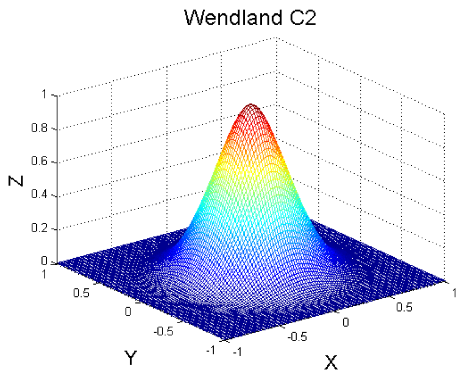
(4) W

Wendland et al. constructed a basis function with a compact support in 1995 [41], which has the following uniform form:

$$\varphi \left(r\right)=\left\{\begin{array}{c}{\left(1-r\right)}^{q}p\left(r\right)0\le r<1\\ 0\mathrm{Otherwise}\end{array}\right.$$

(17)

The RBF in the above form has the following three characteristics:

(a) Compact support

Figure 1 shows the changes in the value of the W basis function with the Euclidean distance. Within the support radius, the impact of the central point and the gradient of the function both gradually decrease as the Euclidean distance increases; outside the support radius, the value of the function is always zero.

(b) Solvability

This basis function can ensure that the constructed coefficient matrix is positively defined and can thereby ensure that there is a unique solution to the matrix equation.

(c) Complexity

The calculation complexity includes three aspects: (1) the time complexity of constructing Equation (13); (2) the time complexity of solving Equation (13); and (3) the time complexity of calculating the function value using Equation (7). For a global basis function, the time complexity of constructing a coefficient matrix A is O(n²). As all the elements on the diagonal lines in the coefficient matrix are zero, and all other elements are non-zero, the spatial complexity is O(n²). When solving Equation (13), some iterative algorithms with limited steps can be used to reduce the complexity to O(n²). The complexity of calculating the interpolation function value is O(n). When a CSRF is used, the coefficient matrix is distributed in a sparse banded pattern, which can significantly reduce the computational complexity. Thus, CSRFs are more suitable for large-scale matrix problems. The TPS RBF and a CSRF are compared in

Table 2. Comparison of the computational complexity.

	TPS Basis Function	CSRF
Time complexity of constructing the coefficient matrix	O(n2)	O(nlogn)
Time complexity of solving the system of linear equations	O(n2)	O(n1.5)
Spatial complexity of storing the coefficient matrix	O(n2)	O(n)
Time complexity of numerically estimating the interpolation function	O(n)	O(logn)

.

4. Application of Basis Functions to 2D Modification Problems

In this section, the G, MQ, TPS, and W functions are selected as basis functions, and their properties are compared through some typical 2D modification problems.

4.1. Curve Modification

(1) Sinusoidal function modification

Five control points (solid circles) are selected from the full cycle of a sinusoidal function from 0 to 4 in the X-axis.

The points at X = 0, 2, and 4 are constrained points. The points at X = 1 and 3 are variable points, whose Y-coordinates change to 0. Additionally, when the Y-coordinate of each point is 0, the graph is considered to be the standard after modification, i.e., the straight line represented by triangles in Figure 2. The four basis functions are used to modify the sinusoidal function. The average error (

Table 3. Comparison of the basis functions in terms of the interpolation error.

Basis Function Type	G	MQ	TPS	W
Average error	0.028233	0.02089	0.04448	0.013

) in the distance between the post-modification graph and the standard graph for each basis function is determined, whose expression is as follows:

$$Error={\displaystyle \sum _{i=1}^n\sqrt{\begin{array}{l}{\left(x_i\left(deformation\right)-x_i\left(standard\right)\right)}^2+\\ {\left(y_i\left(deformation\right)-y_i\left(standard\right)\right)}^2\end{array}}}/n$$

(18)

(2) Semicircle expansion

Five variable points (solid circles) are selected from a semicircle with a radius of 1 and a center at (0, 0). The coordinates of each variable point expand outwardly by 1 in the radial direction. The semicircle with a radius of 2, represented by triangles in Figure 3, is considered to be the standard graph after modification. The four basis functions are used to modify the semicircle. The average errors are compared in

Table 4. Comparison of the basis functions in terms of the interpolation error.

Basis Function Type	G	MQ	TPS	W
Average error	0.05264	0.05309	0.05639	0.05037

.

The smaller the average error is, the closer the post-modification graph is to the standard graph. The modification results for the above two examples demonstrate that the average errors for the W basis function are the smallest, followed by those for the G and MQ basis functions, and finally by those for the TPS basis function. This indicates that the modified graphs obtained using the W basis function are closer to the respective standard graphs, and that the W basis function can preserve the geometric relations in the original graphs to a relatively satisfactory level.

4.2. Grid Point Modification

In this section, the basis functions are compared through grid point modification. The following metrics are introduced to evaluate the modification results [42].

MaxD: This variable represents the maximum distance between the adjacent points of all the grid points, and indicates the increase in the inter-point distance.

MinD: This variable represents the minimum distance between the adjacent points of all the grid points, and indicates the decrease in the inter-point distance.

MaxΔP: This variable represents the maximum displacement of the grid points after modification, and indicates the maximum displacement of a single grid point.

MaxΔD: This variable represents the maximum change in the distances from a grid point to its adjacent points before and after modification, and is used to evaluate the smoothness of the modification.

>0.7MaxΔP: This represents the percentage of the number of grid points that undergo a displacement greater than 70% of MaxΔP after modification to the total number of grid points.

0.3MaxΔP–0.7MaxΔP: This represents the percentage of the number of grid points that undergo a displacement greater than 30% of MaxΔP but less than 70% of MaxΔP after modification to the total number of grid points.

<0.3MaxΔP: This represents the percentage of the number of grid points that undergo a displacement less than 30% of MaxΔP after modification to the total number of grid points.

(1) Grid translation

Four variable points located in the center are selected from 21 × 21 evenly arranged coordinate points and translated over a certain distance along the 45° direction. Four constrained points are selected from the four boundary corners, i.e., their coordinates undergo no change. Figure 4 shows the modification of all the coordinate points obtained by the interpolation (b): G function; (c): MQ function; (d) W function with a support radius of 6 (W6); (e) W function with a support radius of 20 (W20); and (f) TPS. Comparison of the modification results as shown in

Table 5. Comparison of the modification results.

	G	MQ	TPS	W6	W20
MaxD	2.1911	1.71276	2.00393	2.04816	1.79229
MinD	0.52658	0.79142	0.80267	0.57659	0.7475
MaxΔD	0.77688	0.29855	0.58972	0.63395	0.37808
MaxΔP	2.63832	2.27287	2.15464	2.54011	2.35984
>0.7MaxΔP	8.16%	23.58%	59.41%	8.84%	17.23%
0.3MaxΔP−0.7MaxΔP	12.70%	55.56%	34.69%	17.46%	39.00%
<0.3MaxΔP	79.14%	20.86%	5.90%	73.70%	43.76%

.

(2) Grid rotation

Four variable points in the center are selected, and their coordinates are rotated counterclockwise by 45°. Additionally, the displacements of the four points at the boundary corners are constrained. Figure 5 shows the modification of all the coordinate points obtained by the interpolation. Comparison of the modification results as shown in

Table 6. Comparison of the modification results.

	G	MQ	TPS	W6	W20
MaxD	2.1119	1.77723	1.69733	1.90297	1.83995
MinD	0.34665	0.24441	0.42049	0.52243	0.47561
MaxΔD	0.69769	0.36302	0.28311	0.48876	0.42574
MaxΔP	1.60572	1.46266	1.96215	2.03037	2.3984
>0.7MaxΔP	6.35%	23.13%	51.25%	24.94%	39.91%
0.3MaxΔP–0.7MaxΔP	14.06%	57.60%	39.46%	30.39%	45.81%
<0.3MaxΔP	79.59%	19.27%	9.30%	44.67%	14.29%

.

(3) Grid expansion

Four variables in the center are selected, and their coordinates are expanded outward by a certain distance. Additionally, the displacements of the four points at the boundary corners are constrained. Figure 6 shows the modification of all the coordinate points obtained by the interpolation. Comparison of the modification results as shown in

Table 7. Comparison of the modification results.

	G	MQ	TPS	W6	W20
MaxD	2.8853	2.6243	2.60005	2.75483	2.62433
MinD	0.4992	0.84776	0.78768	0.55467	0.68368
MaxΔD	1.47108	1.21008	1.18583	1.34062	1.21011
MaxΔP	2.12132	2.12132	2.40301	2.12132	2.56143
>0.7MaxΔP	9.07%	34.47%	59.86%	13.61%	49.89%
0.3MaxΔP–0.7MaxΔP	15.42%	51.70%	31.75%	19.95%	37.19%
<0.3MaxΔP	75.51%	13.83%	8.39%	66.44%	12.93%

.

(4) Arbitrary grid modification

Six variable points in the center are selected, and their coordinates are changed arbitrarily. Additionally, the displacements of the four points at the boundary corners are constrained. Figure 7 shows the modification of all the coordinate points obtained by the interpolation. Comparison of the modification results as shown in

Table 8. Comparison of the modification results.

	G	MQ	TPS	W6	W20
MaxD	2.35294	2.18277	2.18763	2.26975	2.29662
MinD	0.55562	0.78784	0.78473	0.71122	0.6951
MaxΔD	0.93872	0.76855	0.77342	0.85554	0.8824
MaxΔP	1.09929	1.04655	1.38189	1.32354	1.59489
>0.7MaxΔP	5.67%	7.48%	18.59%	7.03%	12.70%
0.3MaxΔP – 0.7MaxΔP	18.82%	56.69%	68.03%	38.55%	65.53%
<0.3MaxΔP	75.51%	35.83%	13.38%	54.42%	21.77%

.

The above four modification examples demonstrate that the G’s MaxD has a relatively high value, its MinD has a relatively low value, and the changes in the coordinates of the majority of the points are less than 0.3MaxΔP. This suggests that the G RBF modifies a relatively small area relatively intensively (as clearly evidenced in Figure 7b) and fails to achieve a sufficiently smooth outward transition, which is in agreement with the properties of local basis functions.

When the MQ is used, MaxΔP is extremely small and the changes in the coordinates of more than half of the points are between 0.3MaxΔP and 0.7MaxΔP, indicating a relatively large modification-affected area and relatively gentle modification results.

Compared to the other three basis functions, when the TPS is used, the changes in the coordinates of the majority of the points are greater than 0.3MaxΔP, indicating the largest modification area. In addition, there is a relatively small change in the inter-point distance (MaxΔD is relatively small), i.e., the movements of all the points exhibit a relatively uniform trend. When the MQ and TPS are used, the modification area is relatively large. As shown in the relevant figures, the entire graph, including the points on the boundaries, exhibits a consistent modification trend as the control points. This is in agreement with the properties of the global functions.

In this section, the modification results obtained using two W functions with different support radii are compared. When the W6 is used, the modification area is relatively small and concentrated in the center and all the points on the outermost boundaries undergo no displacement. Compared to the local and G, when the W6 is used, MaxΔD becomes smaller, and the number of points with modification over 30% of the maximum value increases, suggesting that the W function results in a gentler transition to the periphery. When the W20 is used, the modification area covers the entire area. Its modification results are similar to those obtained using the TPS, except that MaxΔP is relatively large. See Cheng et al. (2018) for a detailed introduction of support radius.

In summary, the W function is effective in local contraction, compression, and distortion, and can result in a relatively gentle transition to the boundaries and preserve the geometric relations in the original graph to a relatively satisfactory level. Additionally, by adjusting the support radius, the W RBF can have the properties of both local and global basis functions within a certain range and can thus be used flexibly. Furthermore, the W function is compactly supported and solvable and is also advantageous in terms of computational time. Therefore, it is suitable to use the W function as a basis function to modify hull surfaces.

5. Case Study of Hull Surface Modification Based on the W Basis Function

Based on the aforementioned analysis, we developed a hull surface modification module and used it to modify the surface of a standard Series 60 ship model. Series 60 is a typical cargo ship form with no bow, and is recognized by the International Towing Tank Conference as a standard ship form. The ship model used in this study is the same as the model used by the Iowa Institute of Hydraulic Research (IIHR). The ship model has an inter-perpendicular length of 3.048 m and a block coefficient of 0.6. The main scale factors of Series 60 as shown in

Table 9. Main scale factors of the standard ship model, Series 60.

Lpp (m)	Lwl (m)	Bwl (m)	T (m)	Cb	Cm	$\nabla$ (m3)	Swet (m2)
3.048	3.101	0.406	0.163	0.6	0.977	0.1214	1.6

.

Four variable points in the bow are selected and their coordinates are set anew. Additionally, points on the deck lines at the sides, base line, and design waterline are selected as fixed points, as shown in Figure 8. Before the solving process of the support radius using Delaunay triangulation method, these fixed points (on the deck line or on the design line, etc.), should be selected in advance. However, at this time, the size of the support radius is unknown. Therefore, whether these points are within the support radius or outside the support radius, that is, whether these points are affected, is unknown. In order to ensure those points are not affected, they must be selected as fixed points. Matrix F is constructed with the changes in the selected variable and fixed points. Then, matrix A is obtained after using each of the selected points as the interpolation center. By solving Equation (13) in three directions, all the unknown coefficients ${\lambda }_i$ and $c_i$ can be determined. Finally, by substituting the remaining points (unknown points) into Equation (7), the new coordinates of all the unknown points can be obtained, which form a new surface. Figure 8 shows the new ship form obtained by the RBF interpolation. As demonstrated in Figure 8, the lines at the waterline undergo no changes after modification; below the waterline, the bodylines at stations 1–8 are wider and fair after modification.

Similarly, four variables in the bow are selected, and their coordinates are rese; control points on the deck lines at the sides, base line, and some station lines are selected as constrained points, as shown in Figure 9. A new ship form can then be obtained by RBF interpolation. After modification, there are no changes in the lines between stations 5 and 20 in the bow.

In the above examples, the bow of the ship is modified with four design variables alone. This suggests that if proper variable points are selected, the W basis function-based surface modification method can be used to rapidly modify a hull surface with a relatively small number of design variables. In the examples, the fixed points constrain the deck lines at the sides, design waterline, stations, and base line. After modification, there are no changes to the lines at the corresponding locations. This indicates that when it is used to modify a hull surface, the W basis function-based surface modification method can constrain specific locations by selecting fixed points to allow these locations to undergo no changes, which can consequently preserve the specific line form of the parent ship and facilitate the engineer in formulating a general arrangement design.

6. Application Examples

The theoretical explanation of Section 2 and the two-dimensional deformation example of Section 3 are used to select the radial basis function which is the most suitable for the deformation of the hull surface, and finally the W function is selected. Therefore, only the W function was used as the basis function in this section.

The hull surface modification module has been integrated into the multidisciplinary comprehensive optimization platform for the hydrodynamic performance of ships. Here, the trimaran is selected again as the study object. The original trimaran consisted of a slender body in the center and two side bodies symmetrically distributed on either side of the body. The profile of the side bodies was scaled from the main body line at 1:3. The size information of trimaran owners is shown in

Table 10. The size information of trimaran.

	Lwl (m)	B (m)	D (m)	D (m)	Cb	Cm
Main body	4.08	0.45	0.48	0.26	0.397	0.586
Side body	1.36	0.15	0.16	0.09	0.397	0.586

, and its 3D model is shown in Figure 10.

6.1. Description of the Optimization Problem

The optimization objective is defined as follows:

$$f_{obj}=\min C_w,Fn=0.434$$

(19)

(1) Variable selection

In the main and side body line synchronous optimization, variable points are selected on the main body and the side body. As shown in Figure 11, 10 variation points in the main body, numbered 1 to 10, are chosen, with three variation points on the strip numbered 11–13. Point 1 is in the x direction and points 2–13 in the y-direction. The range of design variables is shown in

Table 11. Values of design variables.

Design Variables	Initial Value	Upper Limit of the Variable	Lower Limit of the Variable
X1	0.1356	0.1360	0.1220
Y1	0	0.0100	0
Y2	0.0397	0.0438	0.0358
Y3	0.0714	0.0786	0.0700
Y4	0.1016	0.1118	0.0920
Y5	0.0047	0.0052	0.0044
Y6	0.0213	0.0235	0.0199
Y7	0.0343	0.0378	0.0310
Y8	0.2118	0.2330	0.1910
Y9	0.1974	0.2170	0.1780
Y10	0.2257	0.2483	0.2030
Y11	0.0121	0.0100	0.0150
Y12	0.0371	0.0400	0.0350
Y13	0.0662	0.0720	0.0600

. In the main body, X1 controls the length of water line. Y1–4 are arranged along the waterline to control the size of the inflow angle and shape of the inflow section on the waterline. Y5–7 can have a great effect on the bilge line. Y8–10 control the size of the outflow angle and shape of the outflow section on the waterline. At the side body, Y11–12 control the size of the inflow angle and shape of the inflow section on the waterline. Y13 controls the size of the outflow angle and shape of the outflow section on the waterline.

(2) Constraints

Hydrostatic constraint is the displacement volume ∇ constraint $\frac{{\nabla }_{opti}-\nabla }{\nabla }\ge 0$. In the optimization of the resistance, in order to ensure other performance of the ship, traditionally, the constraint of the drainage volume is generally set to ±1%. However, in this paper, the constraint of the drainage volume is set to be greater than 0, in order to obtain an optimized ship hull with an increased drainage volume and a reduced total resistance.

Line constraint refers to each of the main scale factors (length, width, and draft). These remain unchanged; the outline of the bow and the base line remain essentially unchanged, and some hull stations remain unchanged. Figure 11 shows the fixed points.

Longitudinal position constraints of center of buoyancy is $\left|\frac{Lcb-Lc{b}_{opti}}{Lcb}\right|\le 1.5\%$

(3) Optimization algorithm

The PSO algorithm is selected. The number of iterations is set to 90, with 30 particles in each iteration.

6.2. Analysis of the Optimization Results

Figure 12 shows the optimization results of 2700 groups. In Figure 12, the C_W of the initial ship is marked. The hull form with the lowest C_W is selected.

Table 12. Hydrodynamic data.

Ship Form	∇/m3	Wet Surface Area/m2	Longitudinal Position of Center of Buoyancy/m	Wave Resistance Coefficient (× 10−3)	Total Resistance/N
Initial ship	0.203	2.879	2.52	3.24	81.4
Optimized ship	0.2045	2.894	2.50	2.97	79.2
Change	+0.74%	+0.50%	−0.79%	−8.30%	−3.8%

summarizes the hydrostatic and hydrodynamic data of the initial and optimized ship, respectively. To save time, the SHIPFLOW software wass used in the optimization process to calculate the C_W of the hull. To validate the optimization results, FineMarine software is used to calculate R_t values of the initial and optimized ship after optimization. Compared to the initial ship, the optimized ship has a 0.74% higher ∇, a 0.79% lower center of buoyancy L_cb in the longitudinal direction, a 0.50% higher wet surface area S, an 8.3% lower C_W, and a 3.8% lower R_t.

Figure 13 and Figure 14 show the comparison of the lines of the initial and optimized ships. Figure 15 and Figure 16 show the comparison of wave forms and wave heights, respectively. The comparison of lines clearly shows that, compared with the original ship, the profile of the fixed point has not changed. The forward mid-ship line of the main body and side body becomes fuller, and the rear mid-ship line becomes thinner, thus reducing the wave interference between the main body and the side body.

7. Conclusions

The hull surface modification method plays an important role in the ship form optimization framework. The selection of the basis function is key in the RBF interpolation-based surface modification method. Therefore, this study focused on the selection of the basis function. Based on the theoretical explanations of several typical basis functions and their comparisons through examples, the W function was found to be advantageous. Additionally, the W function interpolation-based surface modification method was used to modify and optimize trimaran ship model. The conclusions are as follows:

(1) The W function has characteristics of both local and global basis functions and is flexible. Additionally, the W function is compactly supported, solvable, and advantageous in terms of its computational time. Thus, the W function is suitable for hull surface modification.

(2) The W function interpolation-based surface modification method can rapidly modify a hull surface with a relatively small number of points, and can allow the lines at corresponding locations of the hull to undergo no changes by selecting fixed points, thereby preserving the special lines of the initial ship and facilitating the formulation of a general arrangement design.

(3) By integrating the W function interpolation-based surface modification method into an optimization platform, an optimized trimaran hull form with fair lines and an improved drag performance can be obtained, thereby validating the feasibility and value of the W function interpolation-based surface modification method for engineering practice.

The following outlook for future research is presented:

(1) In this study, only a few common basis functions are selected, and their parameters are manually set. Additionally, these basis functions are compared based on specific modification problems. In the future, more basis functions, or scenarios in which different parameters are selected for one basis function, can be taken into consideration.

(2) Currently, this method primarily relies on design experience to select the locations of variable points and determine their ranges, which has certain limitations. Improvements are expected in the future.