Generalized Form of the Invariant Imbedding Method and Its Application to the Study of Back-Scattering in Shallow-Water Acoustics

Abstract

A generalized form of the matrix-invariant imbedding method was developed to solve boundary-value problems for coupled systems of Helmholtz-type equations. Within this approach, a boundary-value problem solution can be obtained by solving evolutionary first-order imbedding equations for a matrix-valued function. The proposed method is applied to the solution of coupled equations for mode amplitudes describing the propagation of acoustic waves in a range-dependent shallow-water waveguide. The back-scattering of modes by bathymetry features is investigated, and the coefficients of the modal expansion of the wave reflected by an inhomogeneity in the bottom relief are computed. It is demonstrated that back-scattering is strongly connected with the modal interactions and that the back-scattered field consists of modes with numbers different from the number of the incident mode.

1. Introduction

The solution of sound propagation problems in practical applications of underwater acoustics often results in very intense computations, since areas of interest often extend hundreds or even thousands of kilometers along horizontal directions. In order to handle such large-scale problems, one usually has to neglect certain physical effects (which are considered to be of secondary importance) when simplifying propagation equations. For example, in all models based on the parabolic equations, the back-scattering of sound is not taken into account for the sake of the simplification of the problem and in exchange for the possibility of using marching computational schemes with large step sizes in range [1,2,3]. Another common approach is to neglect the mode-coupling effect when using computational models based on the theory of normal modes [1,4,5,6]. This simplification allows one to uncouple the equations for mode amplitudes, thus greatly simplifying their solution (while retaining their capability of handling many practical problems).

When performing the aforementioned simplifications, it is always necessary to investigate the inaccuracies in the resulting models of sound propagation that arise due to the neglect of certain terms/effects. Such an investigation can be carried out by using numerically exact sound propagation techniques (e.g., [7,8]). Some forty years ago, a method that allows a reformulation of a boundary-value problem (BVP) for the Helmholtz equation (in particular, related to wave propagation and scattering) in the form of an initial-value problem for the first-order Riccati equation was proposed by Babkin and Klyatskin [9]. The latter equation can be solved with efficient marching numerical algorithms, and yet the reformulation allows one to fully take back-scattering effects into account. This technique is known in the literature as the invariant imbedding method.

In this study, we propose a generalization of this method so that it can be applied to a system of coupled Helmholtz equations (or, in the same way, to a Helmholtz equation for an unknown vector function). Within the proposed approach, the BVP for a system of coupled Helmholtz equations is replaced by a matrix Riccati equation, where the unknown quantity is the matrix of reflection coefficients as a function of the right boundary of an inhomogeneous layer. The generalized invariant imbedding method is applied to the investigation of the back-scattering of sound on a bottom-relief inhomogeneity in a shallow-water waveguide (see Figure 1). In the framework of the normal mode theory, the solution of this problem consists in the computation of mode amplitudes satisfying a coupled system of 1D elliptic equations [1]. The proposed method allows us to investigate the interplay between the back-scattering and the mode-coupling effects in a shallow-water environment. The computation of the matrix of reflection coefficients for different incident modes reveals the fact that the back-scattering is always accompanied by strong mode coupling.

It is interesting to note that matrix Riccati equations for reflection coefficients can also be found in the literature in the context of elastic wave propagation [10,11,12]. Although their derivation in the mentioned works follows a different scheme, it appears that such equations can be applied to the simulation of any sort of waves described by a vector-valued function.

2. Problem Statement

The problem of sound propagation in the 2D waveguide of a shallow sea $\Omega =\left\{\right(x,z)\mid z\ge 0\}$ that is depicted in Figure 1 is considered. The waveguide consists of a water layer $0\le z\le h\left(x\right)$ and a liquid-penetrable bottom. These layers are separated by the interface $z=h\left(x\right)$ (the function $h\left(x\right)$ is assumed to be continuous). It is supposed that the water depth h outside the interval $x\in [L_0,L]$ is constant ($h=h_0$). Thus, the bottom-relief inhomogeneity is localized on this interval. Sound propagation in the waveguide $\Omega$ is described by the 2D Helmholtz equation:

$$\frac{{\partial }^{2}P}{\partial x^2}+\frac{{\partial }^{2}P}{\partial z^2}+\frac{{\omega }^2}{c^2}P=0,$$

(1)

where $P(x,z)$ is the acoustic pressure, c is the sound speed, and $\omega$ is the angular frequency.

It is assumed that a normal mode $exp(-i{k}_{0,j}x){\varphi }_{0,j}\left(z\right)$ is incident at the bottom-relief inhomogeneity from the right. Here, ${\varphi }_{0,j}$ is an eigenfunction of the acoustic spectral problem [1]:

$$\left\{\begin{array}{c}{\varphi }_{zz}+\frac{{\omega }^2}{c^2}\varphi -k^2\varphi =0,\hfill \\ \varphi \left(0\right)=0,\hfill \\ \varphi \left(H_{max}\right)=0,\hfill \\ {\varphi |}_{z\to h+0}{=\varphi |}_{z\to h-0},\hfill \\ {\left.\frac{1}{\rho }{\varphi }_z\right|}_{z\to h+0}={\left.\frac{1}{\rho }{\varphi }_z\right|}_{z\to h-0},\hfill \end{array}\right.$$

and $k_{0,j}$ is the corresponding horizontal wavenumber, $\rho$ denotes the density (note that there is usually a density jump at the water–bottom interface), and $H_{max}$ is a sufficiently large value of depth at which the computational domain is truncated (so that this value does not actually influence the simulation results). Throughout this paper, we assume that the mode functions are normalized, i.e., that $\int \frac{{\varphi }_j\left(z\right){\varphi }_{\ell }\left(z\right)}{\rho \left(z\right)}dz={\delta }_{j\ell }$ (hereafter, the integration with respect to z is always performed along the interval $[0,H_{max}]$).

The solution of Equation (1) in the waveguide can be represented [1] in the form of a truncated modal expansion (hereinafter, only the first n modes are taken into account)

$$P(x,z)=\sum _{j=1}^n{A}_j\left(x\right){\varphi }_j(x,z)$$

(2)

where ${\varphi }_j(x,z)$ are eigenfunctions obtained from (2) for a fixed value of x, and $A_j\left(x\right)$ are mode amplitudes satisfying the following coupled system of equations:

$$\frac{{\partial }^2{A}_j\left(x\right)}{\partial x^2}+k_j^2\left(x\right)A_j+\sum _{l=1}^n{U}_{lj}{A}_l+2\sum _{l=1}^n{V}_{lj}\frac{\partial A_l}{\partial x}=0,$$

(3)

where $U_{lj}=\int \frac{{\partial }^2{\varphi }_l}{\partial x^2}\frac{{\varphi }_j}{\rho }dz,$ and $V_{lj}=-V_{jl}=\int \frac{\partial {\varphi }_l}{\partial x}\frac{{\varphi }_j}{\rho }dz$ are elements of the square $n\times n$ matrices $\mathit{U}$ and $\mathit{V}$, respectively.

The set of n scalar equations (3) can be replaced by a single equation for the unknown vector function $\mathit{a}\left(x\right)={(A_1\left(x\right),A_2\left(x\right),\dots ,A_n\left(x\right))}^T$:

$$\left(\frac{d^2}{d{x}^2}+\mathbf{\Gamma }\left(x\right)\frac{d}{dx}\right)\mathit{a}\left(x\right)-\mathit{Q}\left(x\right)\mathit{a}\left(x\right)=0,$$

(4)

where $\mathbf{\Gamma }\left(x\right)=2\mathit{V}\left(x\right)$, $\mathit{Q}\left(x\right)=-{\left(\mathit{K}\left(x\right)\right)}^2-\mathit{U}\left(x\right)$, and $\mathit{K}=\mathrm{diag}(k_1\left(x\right),\dots ,k_n\left(x\right))$ (i.e., $\mathit{K}\left(x\right)$ is a diagonal matrix with eigenvalues $k_j\left(x\right)$ on the main diagonal).

In order to formulate a BVP for Equation (4), we derive the boundary conditions at $x=L_0$ and $x=L$ in the case of incidence of a single normal mode at the right boundary of the inhomogeneous section of the waveguide $\Omega$. In what follows, we write ${\mathit{a}}_l(x;L)$ instead of $\mathit{a}\left(x\right)$, emphasizing the dependence of the solution on the position of the right boundary (in accordance with the notation used in [9]). The subscript l corresponds to the number of the incident mode. In addition, it is supposed that time dependence is suppressed in such a way that $e^{ikx}$ corresponds to propagation in the positive direction of the X axis [1].

Since the field for $x\ge L$ is a superposition of the l-th incident normal mode and back-scattered wave consisting of all modes taken into account, the vector $\mathit{a}(x;L)$ can be represented in the following form:

$${\mathit{a}}_l=\left(\begin{array}{c}{R}_{1,l}{e}^{i{k}_1(x-L)}\\ R_{2,l}{e}^{i{k}_2(x-L)}\\ ⋮\\ R_{l,l}{e}^{i{k}_l(x-L)}+e^{-i{k}_l(x-L)}\\ ⋮\\ R_{n,l}{e}^{i{k}_n(x-L)}\end{array}\right),$$

(5)

where $R_{p,q}$ are reflection coefficients to be computed.

For $x\le L_0$, the vector $\mathit{a}(x;L)$ can be written in the form

$${\mathit{a}}_l=\left(\begin{array}{c}{T}_{1,l}{e}^{-i{k}_1(x-L_0)}\\ T_{2,l}{e}^{-i{k}_2(x-L_0)}\\ ⋮\\ T_{l,l}{e}^{-i{k}_l(x-L_0)}\\ ⋮\\ T_{n,l}{e}^{-i{k}_n(x-L_0)}\end{array}\right),$$

(6)

where $T_{p,q}$ are transmission coefficients. It is easy to see that $\mathit{a}(x;L)$ given by (5) and (6) satisfies the following boundary conditions at $x=L$ and $x=L_0$:

$$\begin{array}{c}\frac{\partial }{\partial x}\mathit{a}\left(L_0\right)+i{\mathit{K}}_0\mathit{a}\left(L_0\right)=0,\hfill \\ \frac{\partial }{\partial x}\mathit{a}\left(L\right)+i{\mathit{K}}_0\mathit{a}\left(L\right)=\left(\begin{array}{c}0\\ ⋮\\ -2i{k}_l\\ ⋮\\ 0\end{array}\right),\hfill \end{array}$$

(7)

where ${\mathit{K}}_0\equiv \mathit{K}\left(L\right)=\mathit{K}\left(L_0\right)$, and the elements of the vector on the right-hand side of the second condition are all zeros, except for the l-th one.

The boundary conditions (7) and the vector Helmholtz Equation (4) can be considered as a vector boundary-value problem. All n column vectors ${\mathit{a}}_l(x;L)$ can be combined into a square matrix $\mathit{A}(x;L)$ that satisfies the matrix boundary-value problem

$$\begin{array}{cc}\hfill & \left(\frac{d^2}{d{x}^2}+\mathbf{\Gamma }\left(x\right)\frac{d}{dx}\right)\mathit{A}\left(x;L\right)-\mathit{Q}\mathit{A}\left(x;L\right)=0,\hfill \\ \hfill & \mathit{B}\left(L_0;L\right)\hspace{0.17em}+\hspace{0.17em}{\mathit{D}}_0\mathit{A}\left(L_0;L\right)\hspace{0.17em}=\hspace{0.17em}\mathbf{0},\hfill \\ \hfill & \mathit{B}\left(L;L\right)\hspace{0.17em}+\hspace{0.17em}{\mathit{D}}_2\mathit{A}\left(L;L\right)\hspace{0.17em}=\hspace{0.17em}-2i{\mathit{K}}_0,\hfill \end{array}$$

(8)

where $\mathit{B}=\frac{\partial \mathit{A}(x;L)}{\partial x}$, ${\mathit{D}}_2=-{\mathit{D}}_0$, and ${\mathit{D}}_0=i{\mathit{K}}_0$ (i.e., both ${\mathit{D}}_0$ and ${\mathit{D}}_2$ are diagonal matrices).

In order to simplify the derivation, the solution of the boundary-value problem with the transformed right part of the second boundary condition will be sought.

$$\begin{array}{cc}\hfill & \left(\frac{d^2}{d{x}^2}+\mathbf{\Gamma }\left(x\right)\frac{d}{dx}\right)\tilde{\mathit{A}}\left(x;L\right)-\mathit{Q}\tilde{\mathit{A}}\left(x;L\right)\hspace{0.17em}=\hspace{0.17em}0,\hfill \\ \hfill & \tilde{\mathit{B}}\left(L_0;L\right)\hspace{0.17em}+\hspace{0.17em}{\mathit{D}}_0\tilde{\mathit{A}}\left(L_0;L\right)\hspace{0.17em}=\hspace{0.17em}\mathbf{0},\hfill \\ \hfill & \tilde{\mathit{B}}\left(L;L\right)\hspace{0.17em}+\hspace{0.17em}{\mathit{D}}_2\tilde{\mathit{A}}\left(L;L\right)\hspace{0.17em}=\hspace{0.17em}-\mathit{E},\hfill \end{array}$$

(9)

where $\mathit{E}$ is in the $n\times n$ identity matrix. The solution of the original boundary-value problem (8) can be found using the formula

$$\mathit{A}=2i{\mathit{K}}_0\tilde{\mathit{A}}.$$

(10)

Hereinafter, the tilde symbols are suppressed.

In order to obtain the imbedding equations for the BVP (9), we differentiate it with respect to the parameter L (following the same derivation scheme as that used by Babkin and Klyatskin [9] in the scalar case).

$$\begin{array}{cc}\hfill & \left(\frac{d^2}{d{x}^2}+\mathbf{\Gamma }\left(x\right)\frac{d}{dx}\right)\frac{\partial \mathit{A}\left(x;L\right)}{\partial L}-\mathit{Q}\left(x\right)\frac{\partial \mathit{A}\left(x;L\right)}{\partial L}=0,\hfill \\ & \frac{\partial \mathit{B}\left(L_0;L\right)}{\partial L}+{\mathit{D}}_0\frac{\partial \mathit{A}\left(L_0;L\right)}{\partial L}=0,\hfill \\ \hfill & \frac{\partial \mathit{B}\left(x;L\right)}{\partial L}\left|{}_{x\to L}\right.+{\mathit{D}}_2\frac{\partial \mathit{A}\left(x;L\right)}{\partial L}\left|{}_{x\to L}\right.=-\frac{\partial }{\partial x}\mathit{B}\left(x;L\right)\left|{}_{x\to L}-{\mathit{D}}_2\mathit{B}(L,L)\right..\hfill \end{array}$$

(11)

Using the system (9) and the second boundary condition, we obtain

$$\begin{array}{cc}\hfill & \left(\frac{d^2}{d{x}^2}+\mathbf{\Gamma }\left(x\right)\frac{d}{dx}\right)\frac{\partial \mathit{A}\left(x;L\right)}{\partial L}-\mathit{Q}\left(x\right)\frac{\partial \mathit{A}\left(x;L\right)}{\partial L}=0,\hfill \\ & \frac{\partial \mathit{B}\left(L_0;L\right)}{\partial L}+{\mathit{D}}_0\frac{\partial \mathit{A}\left(L_0;L\right)}{\partial L}=0,\hfill \\ \hfill & \frac{\partial \mathit{B}\left(x;L\right)}{\partial L}\left|{}_{x\to L}\right.+{\mathit{D}}_2\frac{\partial \mathit{A}\left(x;L\right)}{\partial L}\left|{}_{x\to L}\right.=-\left(\mathbf{\Gamma }\left(L\right)-{\mathit{D}}_2\right)-\left(\mathit{Q}\left(L\right)+\left(\mathbf{\Gamma }\left(L\right)-{\mathit{D}}_2\right){\mathit{D}}_2\right){\mathit{A}}_L.\hfill \end{array}$$

(12)

where, by definition, ${\mathit{A}}_L\equiv \mathit{A}(L,L)$ (similarly, ${\mathit{B}}_L\equiv \mathit{B}(L,L)$). If we compare the last BVP with the problem (9), we can see that their solutions are connected by the following relation:

$$\frac{\partial \mathit{A}\left(x;L\right)}{\partial L}=\mathit{A}\left(x;L\right)\left[\mathbf{\Gamma }\left(L\right)-{\mathit{D}}_2+\left(\left(\mathbf{\Gamma }\left(L\right)-{\mathit{D}}_2\right){\mathit{D}}_2+\mathit{Q}\left(L\right)\right){\mathit{A}}_L\right],$$

(13)

which can be considered as an ordinary differential equation with independent variable L. Its initial condition can be written as

$$\mathit{A}\left(x;L\right)\left|{}_{L=x}=\right.\mathit{A}\left(x;x\right)={\mathit{A}}_x.$$

(14)

The last thing that we need is the equation for the function $\mathit{A}\left(L;L\right)\hspace{0.17em}\equiv \hspace{0.17em}{\mathit{A}}_L$. Let us differentiate this matrix-valued function:

$$\frac{d}{dL}\mathit{A}\left(L;L\right)\hspace{0.17em}=\hspace{0.17em}\frac{\partial }{\partial L}\mathit{A}\left(x;L\right)\left|{}_{x\to L}\right.+\frac{\partial }{\partial x}\mathit{A}\left(x;L\right)\left|{}_{x\to L}\right.=\frac{\partial \mathit{A}\left(x;L\right)}{\partial L}\left|{}_{x\to L}\right.+{\mathit{B}}_L.$$

The last equation can be transformed into a new one by using (12) and (13).

$$\frac{d}{dL}{\mathit{A}}_L={\mathit{A}}_L\left[\left(\mathbf{\Gamma }\left(L\right)-{\mathit{D}}_2\right){\mathit{D}}_2+\mathit{Q}\left(L\right)\right]{\mathit{A}}_L-{\mathit{A}}_L{\mathit{D}}_2-{\mathit{D}}_2{\mathit{A}}_L+{\mathit{A}}_L\mathbf{\Gamma }\left(L\right)-\mathit{E},$$

(15)

The equation can be considered as a matrix Riccati equation. The initial condition for the equation can be obtained from the boundary conditions (12).

$${\mathit{A}}_{L_0}=\mathit{A}\left(L_0;L_0\right)={\left({\mathit{D}}_0-{\mathit{D}}_2\right)}^{-1}.$$

(16)

From (5) and (10), a formula for the reflection coefficients can be derived:

$$\mathit{R}\left(L\right)=2i{\mathit{K}}_0{\mathit{A}}_L-\mathit{E}.$$

(17)

Note that for $n=1$ (that is, when the mode coupling is neglected), the derived imbedding Equations (13) and (15) reduce to their scalar counterparts proposed by Babkin and Klyatskin [9].

Both imbedding Equations (13) and (15) can be easily solved, e.g., with a Runge–Kutta method (the fact that the unknown function is matrix-valued does not lead to any additional complications). Matrices $\mathit{U}$ and $\mathit{V}$ can be easily computed by using formulae for the derivatives of the eigenfunctions with respect to the media parameters [13,14]. The formulae for the first-order derivatives from the earlier work of Godin [13] are more general and allow one to handle multiple interfaces, as well as range-dependent sound speed and density profiles. The main advantage of the approach from the recent study [14] is the possibility to obtain high-order derivatives with respect to h (the formulae for the first-order derivatives from [14] are equivalent to their counterparts from [13]).

3. Modal Decomposition of the Back-Scattering Field: Numerical Results

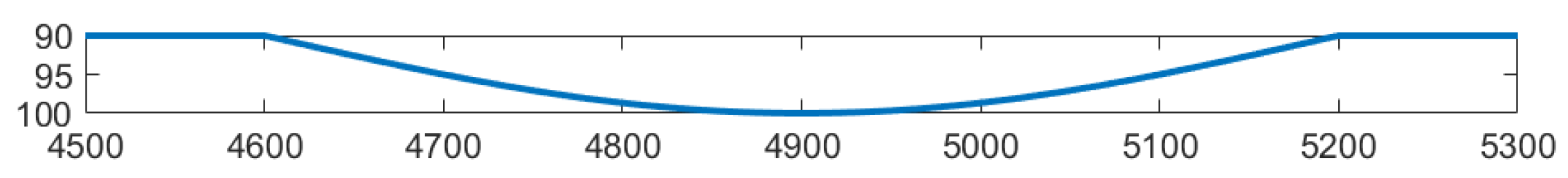
An example of a waveguide with the following parameters is considered. The water depth $h_0$ outside the inhomogeneity is equal to 90 m. The sound speed in the water is $c_1=1500\hspace{0.17em}\mathrm{m}/\mathrm{s}$, and the sound speed in the bottom is $c_2=2000\hspace{0.17em}\mathrm{m}/\mathrm{s}$. It is assumed that the density of the water is ${\rho }_1=1\hspace{0.17em}{\mathrm{g}/\mathrm{cm}}^3$ and the density of the bottom is ${\rho }_2=2\hspace{0.17em}{\mathrm{g}/\mathrm{cm}}^3$. The frequency of the source is $f=50\hspace{0.17em}\mathrm{Hz}$. The lower boundary of the computational domain was set to $H_{max}=200\hspace{0.17em}\mathrm{m}$. For the specified problem parameters, the source excites four waterborne modes for $h=h_0$. We first take into account 20 modes excited by the source, and this number is sufficient to ensure the convergence of the obtained solution.

The depth change associated with the inhomogeneity is varied from 1 to 10 m. The profile of the bottom-relief inhomogeneity is described by the formula

$$h\left(x\right)=h_0+\Delta hsin\left(\pi \frac{x-L_0}{L-L_0}\right),$$

(18)

where $L_0=4600$ m and $L=5200$ m. This is shown in Figure 2.

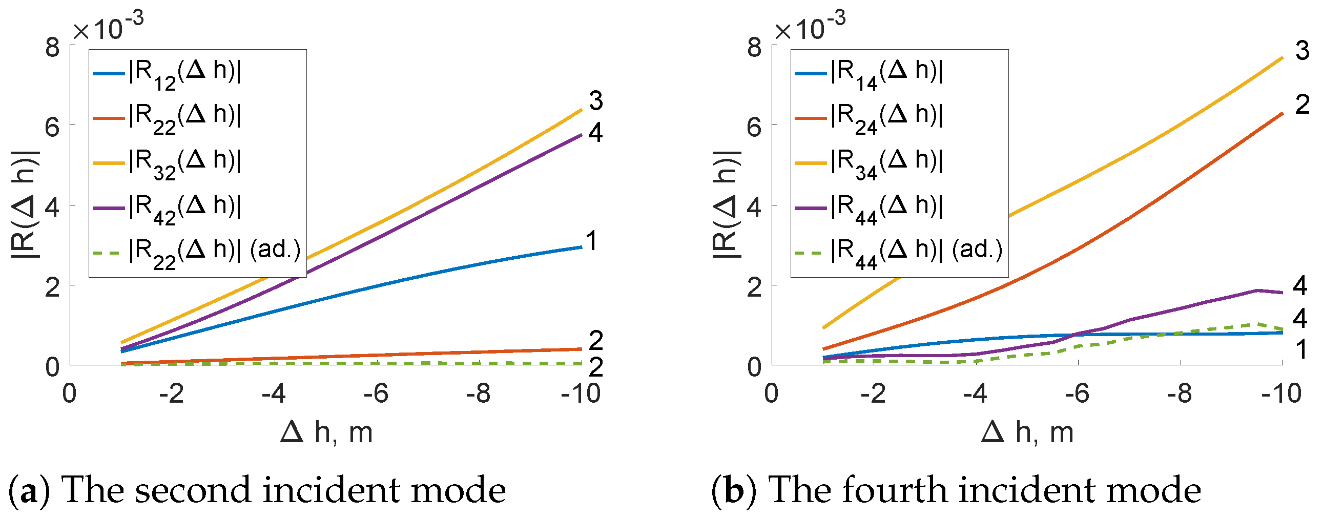
Figure 3a was obtained for the second incident mode. The solid lines represent the excitation of different modes in the reflected field, and the dashed line represents the reflection coefficient computed under the adiabatic assumption (that is, neglecting the mode coupling).

It is easy to see that the values of non-adiabatic reflection coefficient are much larger than the respective quantities obtained in the adiabatic approximation. In addition, the incident modes excite modes with different numbers in the reflected field (the reflected amplitude of the incident mode is relatively small). Thus, we conclude that the back-scattering of acoustic waves in range-dependent environments cannot be considered separately from the mode-coupling effect.

Note that, in fact, all coefficients have relatively small values, since the back-scattering in shallow-water environments with smooth bathymetry variations is not very pronounced. In Figure 3b (which corresponds to the incidence of the fourth mode), one can see that the relations between the values of the reflection coefficients are similar.

The second example of a waveguide is shown in Figure 4. The waveguide has the same parameters, but the depth of the inhomogeneity is varied from −1 to −10 m. Basically, this is a small underwater mountain.

Figure 5a,b were created for this case.

The relations between the mode amplitudes in the reflected field are almost the same as those in the previous example. Again, the energy of the incident modes transforms into the energy of modes with other numbers in the reflected field.

4. Conclusions

In this study, we generalized the invariant imbedding method to the case of a BVP for a vector function. In this case, the derivation results in imbedding equations for a matrix-valued function. In particular, we obtained a matrix Riccati equation for the reflection coefficients. The solution of this equation can be easily obtained with standard ODE integration tools, e.g., with numerical Runge–Kutta schemes. Note that, in the present work, we restricted our attention to the computation of the reflection coefficients from the solution of Equation (15), whereas the computation of the mode amplitudes also requires the solution of Equation (13) (together, they are called imbedding equations by the analogy with the respective scalar equations from the pioneering work [9]). Note that the former is a nonlinear first-order ODE for a matrix-valued function, while the latter equation is linear and, therefore, much easier to solve. We do not present its solution here, as the magnitude of the back-scattered field would anyway be too small to see against the forward-propagating wave (it would be interesting, however, to compute the field, e.g., in 3D environments with rotational symmetry in the horizontal plane by using our approach).

The generalized invariant imbedding method proposed here was applied to the investigation of the modal content of a back-scattered acoustic field in a waveguide with a bottom-relief inhomogeneity. More precisely, we obtained the imbedding equations describing coupled mode amplitudes and computed the modal decomposition coefficients for the reflected field in the case in which the incident wave consisted of a single normal mode. Our results indicate that back-scattering is inevitably accompanied by strong mode coupling, and the reflected field is mostly formed by modes that are different from the incident one. In particular, the latter fact implies that one can always opt for a one-way propagation model once the adiabatic approximation is invoked.

Although in the idealized example considered here, back-scattering occurs only due to the variations in the water depth, the proposed technique can be also used in the case of more realistic environments with a lossy bottom, multiple interfaces (i.e., several layers of the bottom with finite jumps in sound speed and density at the respective boundaries), and range-dependent sound speed profiles. Such cases will be studied in future work. It would be also interesting to use the generalized invariant imbedding equations to solve 3D sound propagation problems in shallow-water waveguides.