Three-Dimensional Sound Propagation in the South China Sea with the Presence of Seamount

Abstract

Seamounts have important effects on sound propagation in deep water. A sound propagation experiment was conducted in the South China Sea in 2016. The three-dimensional (3D) effects of a seamount on sound propagation are observed in different propagation tracks. Ray methods (BELLHOP N×2D and 3D models) are used to analyze and explain the phenomena. The results show that 3D effects have obvious impacts on a sound field within a horizontal refraction zone behind the seamount because some sound beams cannot reach the receiver for the horizontal refraction effects, which impacts the sound field within a certain angle range behind the seamount. The arrival structure results show that the eigenrays after horizontal reflection will arrive at the receiver earlier than those obtained from the two-dimensional (2D) model within the horizontal refraction zone behind the seamount. This means that the horizontal reflection effect of a seamount will cause the shortening of sound propagation paths. Finally, in the reflection zone in front of the seamount, the 2D and 3D TL results show that the shape of the reflection zone is similar to an “arch” type, and the horizontal refraction of sound waves has little effect on the TLs in the reflection zone of a seamount.

1. Introduction

Seamounts have important effects on sound propagation. Physical experiments and theoretical approaches have been explored over the past several decades. Since the effects of seamounts are complex and the efficiency of numerical methods is usually low, previous studies on the sound propagation of seamounts mostly used 2D or N×2D models. With the deepening of ocean acoustics research, the focus gradually shifted to research about the 3D sound propagation phenomena of seamounts [1,2,3,4,5,6,7,8,9].

Weston proposed the concept of horizontal refraction first and found that continental slopes and seamounts would cause strong horizontal refraction effects [1]. Since then, many scholars tried to explain the physical mechanism of the horizontal refraction phenomena.

Harrison found that horizontal curvature of long-range underwater sound rays can be caused by repeated reflection from a sloping or undulating seabed [2,3]. Ray invariants are used to calculate the horizontal projection of ray paths analytically. Analytical ray paths and shadow zone boundaries are derived for some bottom topographies, including wedges, ridges, and seamounts.

The experiments were carried out near Dickins Seamount in the northeast Pacific Ocean in 1975 [4,5] using explosive shots and CW sources. The results showed that the TL increased up to about 15 dB because the deep refracted waves would be blocked by the seamount, and the shadowing loss behind seamount was an f^1/2 dependence at frequencies greater than 50 Hz.

Kim studied the mechanisms of sound propagation around seamounts [6]. The BASSEX experiment carried out in the Northeast Pacific around the Kermit Roosevelt seamounts in 2004 measured the broadband pulses and found that the convergence and shadow zones behind the seamounts were matched well between the experiment data and 3D sound propagation model results. The reconciliation of the broadband pulses behind the seamount was challenging because of the complicated environment.

A spectral coupled mode model developed by Luo [7] was applied to analyze the propagation and scattering around conical seamounts. The numerical results showed that the shadow zone behind the seamount was broadened by horizontal refraction when the azimuthal variation was strong, and azimuthal coupling could not be ignored.

The propagation experiment was conducted in 2014 in the South China Sea with a flat bottom and a seamount by using explosive sources [8]. The effects of seamounts on sound propagation were analyzed using broadband signals. It was observed that the transmission losses (TLs) decreased up to 7 dB for the signals in the first shadow zone due to seamount reflection. Moreover, the TLs might have increased more than 30 dB in the convergence zone due to the shadowing by the seamounts.

The 3D effects of the seamounts on sound propagation were investigated in a sound propagation experiment which was conducted in the South China Sea in 2016 [9]. The experimental sound field structure behind the seamount was obviously different from the N×2D model’s numerical results. The width of the shadow zone, based on the experimental data, was wider than that calculated by the N×2D model, and the TLs calculated by the N×2D model was about 10 dB less than the experimental results in the horizontal refraction zone. This was because some of the sound beams could not reach the receiver as a result of the horizontal refraction effects, which led to the experimental TLs being larger than the numerical results calculated by the N×2D model. However, the 3D effects of seamounts on the arrival structures and reflection zone were not studied.

In this paper, a sound propagation experiment around the seamount conducted in the South China Sea in 2016 is introduced first. Secondly, the mechanisms of some 3D sound propagation phenomena of the seamount in deep water are analyzed by using N×2D and 3D ray models. In the end, we make a conclusion.

2. Experiment Description

In 2016, an experiment of sound propagation was conducted in the deep water seamount area of the South China Sea. The configuration of the experiment is shown in Figure 1. The vertical linear array (VLA) made up of 20 hydrophones and distributed underwater signal recorders (USRs) from 123 m to 1960 m with different intervals was moored at the bottom, and the depths of the hydrophones were 123 m, 164 m, 203 m, 241 m, 281 m, 322 m, 398 m, 440 m, 482 m, 525 m, 608 m, 723 m, 827 m, 931 m, 1036 m, 1128 m, 1243 m, 1551 m, 1869 m, and 1961 m. The sensitivity of the hydrophones was −170 dB. The sample rate of the hydrophones was 16 kHz. The speed of Shi Yan 1 of the Institute of Acoustics at the Chinese Academy of Sciences was about 10 kn. The wide band signals (WBSs) charged with 1 kg TNT were dropped every 6 min (about every 1.85 km) along different propagation tracks, which were the trajectories of the ship. The nominal detonation depth of the WBSs was 200 m.

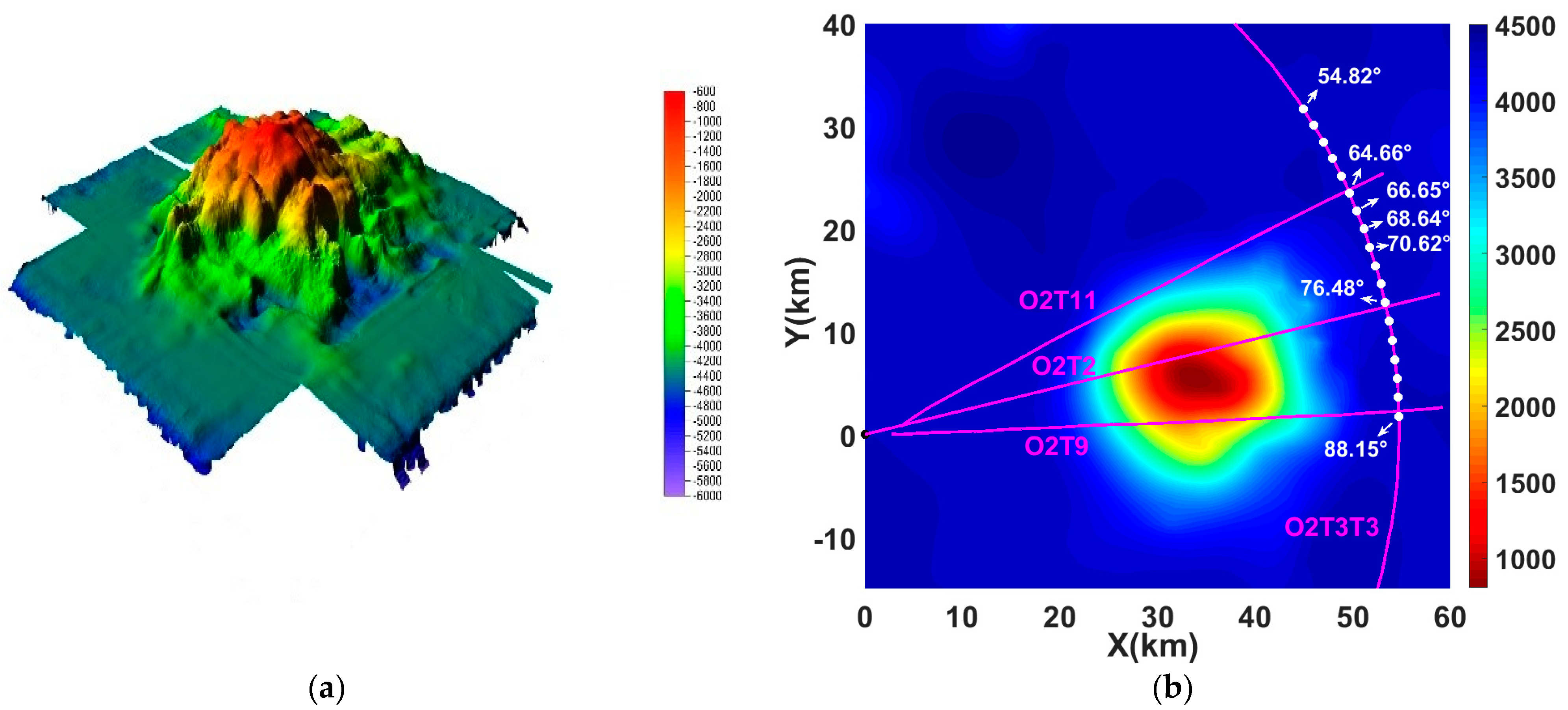
Figure 2a provides the 3D bathymetries measured by a multibeam echosounder in the experiment, but the data were incomplete. Figure 2b gives the 3D bathymetries combined with a database, and the propagation tracks marked by solid pink lines are the trajectories followed by the ship during the experiment, which include the O2T3T3 track that made a circle around the receiver with the distance of the first convergence zone (about 55 km) as the radius. Since the main purpose of the research was to study the 3D effect of a seamount on sound propagation, only part of the O2T3T3 track behind the seamount was applied in the research. In the experiment, the O2T11 track, the O2T2 track, and the O2T9 track passed through the seamount area. It can be found that the top of the seamount along the O2T2 track was about 1000 m below the sea surface and about 33 km from the receiving array. The smallest seabed depth along the O2T11 and O2T9 tracks was about 3300 m and 1500 m, respectively. The average depth of the flat seabed was about 4350 m. Figure 2b also illustrates that the positions of the WBSs measured by a GPS within the range of 54.82–88.15° at the O2T3T3 track, which are marked by white dots. Since the distances between the sound sources and the receiver were basically same, the signals at the O2T3T3 track behind the seamount could be applied to study the 3D effect. The sound sources at 54.82°, 66.65° and 70.62° were used to investigate the 3D effect of the seamount on the arrival structures of the sound signals.

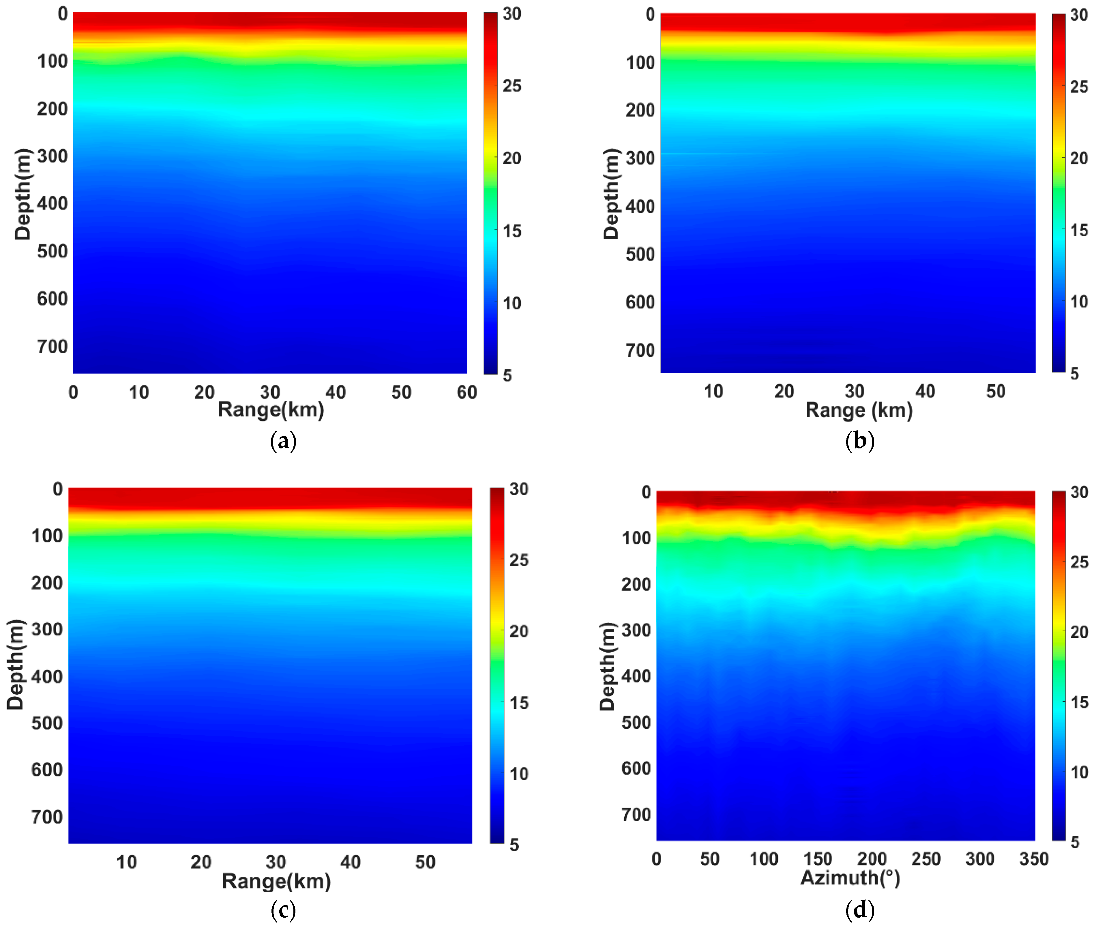
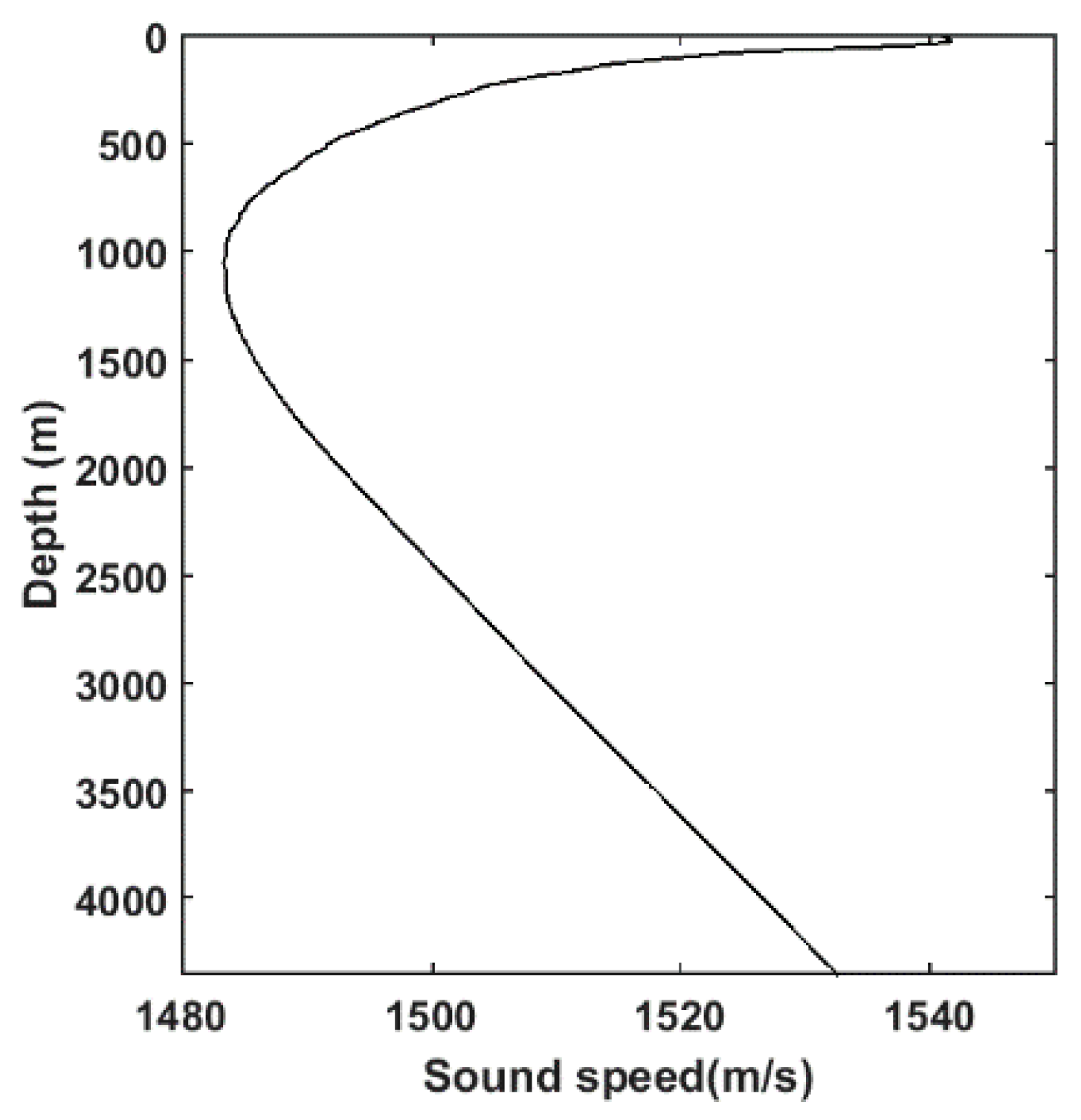
The Expendable Bathy Thermograph (XBT) sensors were used to measure the temperature profiles along the propagation tracks every 10 km. The results in Figure 3 show the variation of the seawater temperature with the depth, distance and azimuth along the O2T2, O2T11, O2T9, and O2T3T3 tracks. It can be found that there was no abnormal heterogeneity during the experiment and the temperature profiles in different tracks were stable and similar. Thus, this was a range-independent environment for the sound speed profile of the water volume during the experiment. The sound speed profile showed in Figure 4 was measured with the Expendable Conductivity Temperature Depth (XCTD) system casted near the receiving array in the experiment. This could be used to calculate the 3D sound field because of the range-independent environment. The depth of the sound channel axis was about 1050 m, and the sound speed at the deepest depth in the water column was 1533 m/s, which was less than that at the sea’s surface (1541 m/s).

The experimental transmission losses (TLs) could be calculated by signal processing [8]. The measured spectrums were averaged in a 1/3-octave bandwidth. The narrow band energy of the propagation signal is represented as

$$E\left(f_0\right)=\frac{2}{F{s}^2}\frac{1}{n{f}_2-n{f}_1+1}{{\displaystyle \sum }}_{i=n{f}_1}^{n{f}_2}{\left|X_i\right|}^2,$$

(1)

where X_i represents the FFT spectrum of the signal x(t) at the ith frequency bin, $f_0$ is the central frequency, F_s is the sample rate, and nf₁ and nf₁ are the start and end frequency numbers for the frequency band, respectively.

The transmission loss (TL) can be denoted as

$$TL\left(f_0\right)=S\left(f_0\right)-\left(10\log \left(E\left(f_0\right)\right)-b\right),$$

(2)

where S is the source level and b is the sensitivity of the hydrophones.

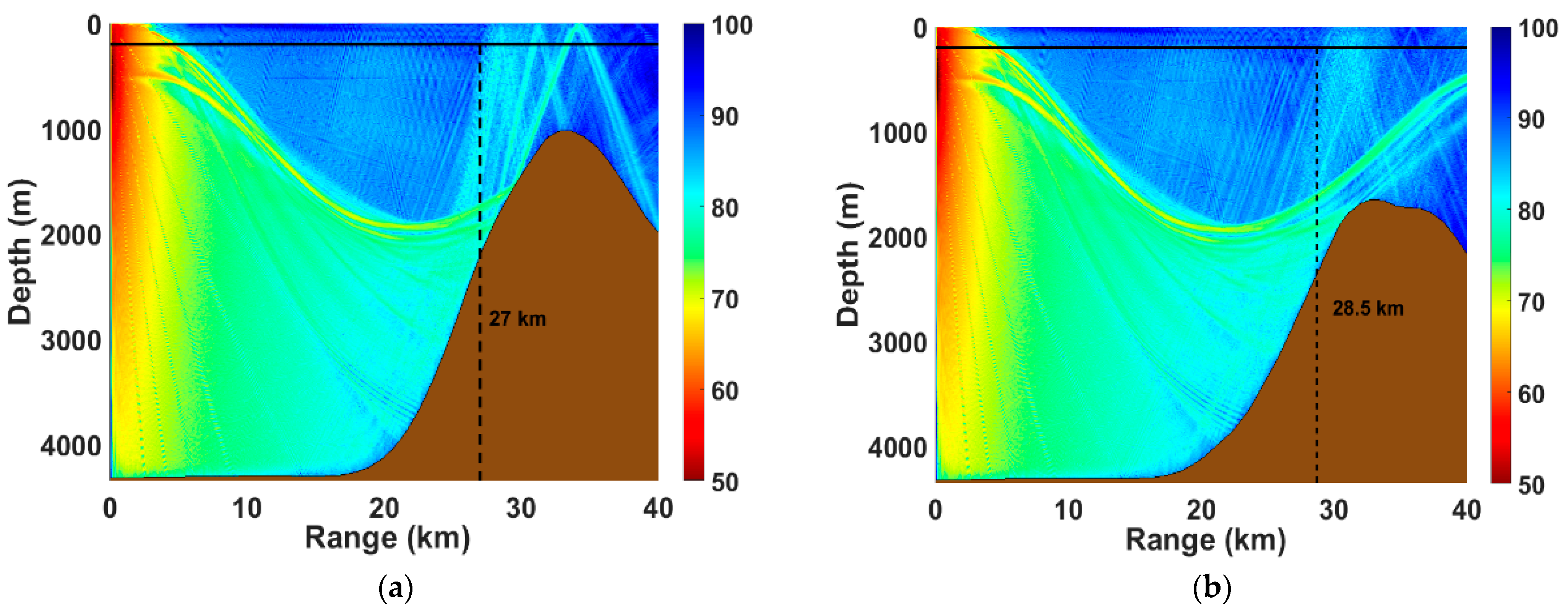
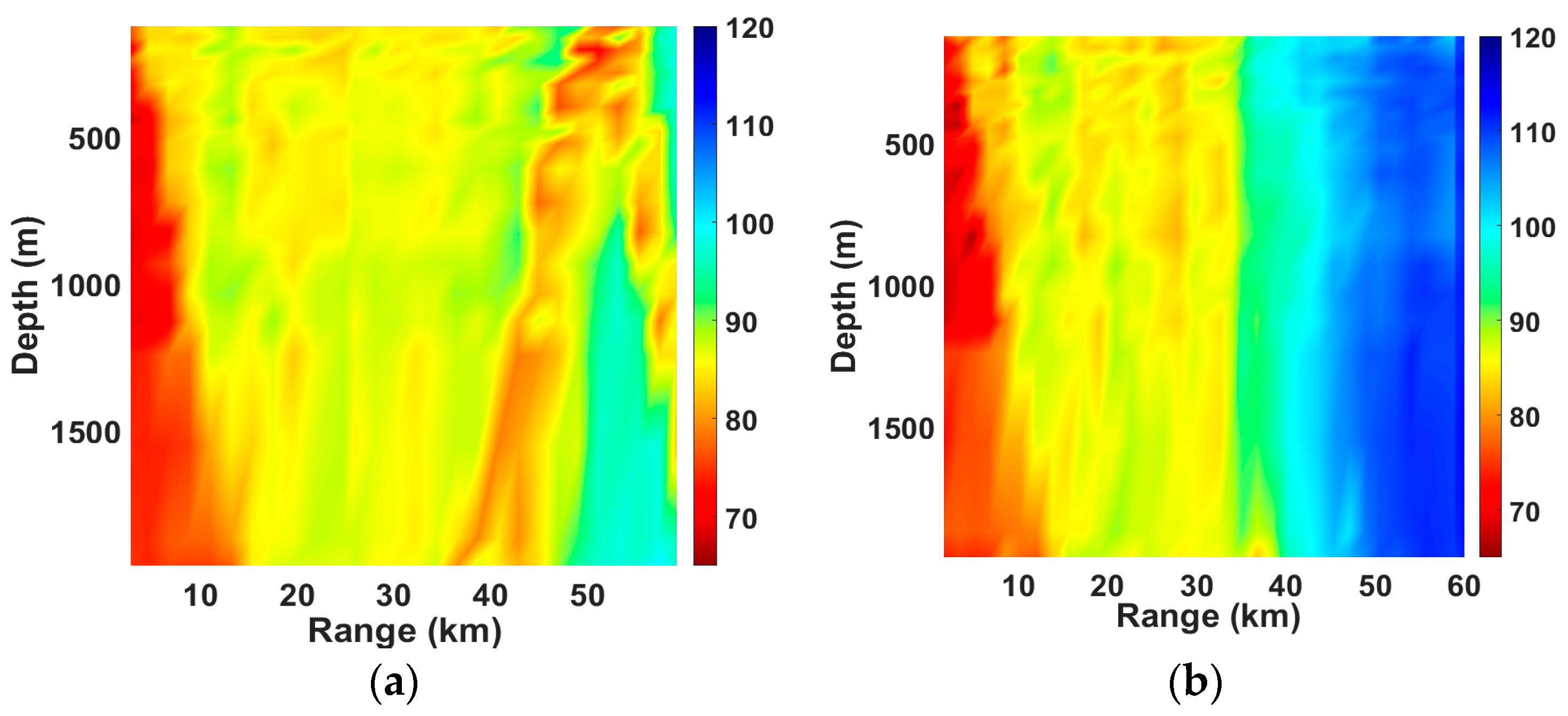
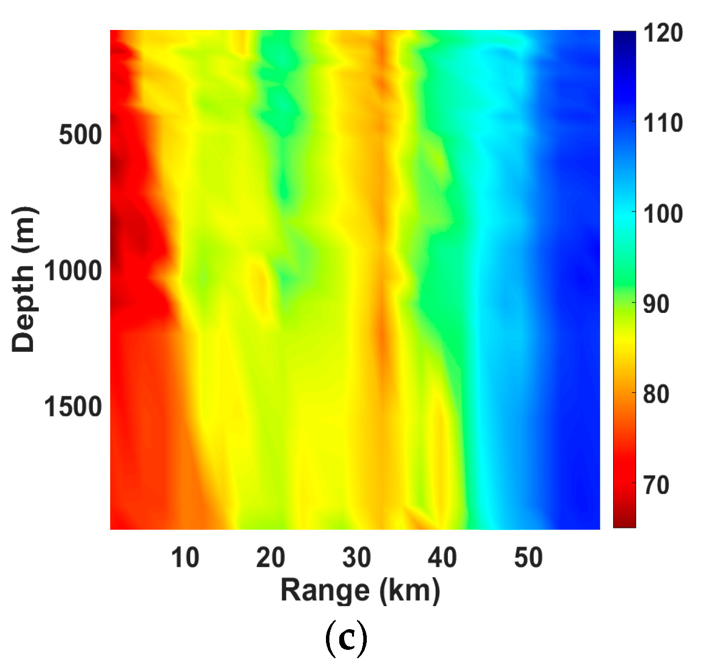
The experimental TL results of the O2T11, O2T2, and O2T9 tracks are given in Figure 5, where the central frequency was 300 Hz and the receiver depths varied from 123 m to 1960 m. It can be observed that the experimental TL results were different along the O2T11, O2T2, and O2T9 tracks passing through the seamount area. In the O2T11 track, the convergence zone structure of the deep sea was not destroyed, which indicates that the direct waves from the source were not completely blocked by the seamount because the height of the seamount in the O2T11 direction was not high enough. In the O2T2 and O2T9 tracks, the existence of a seamount caused destruction of the convergence zone because sound energy was shadowed by the seamount and formed the acoustic shadow zone behind the seamount, which made the TLs behind the seamount increase more than 30 dB [8]. It could also be found that the experimental TL results decreased up to about 7 dB in the range of about 27–35 km in front of the seamount in the O2T2 and O2T9 tracks due to the seamount reflection, which is in good agreement with the conclusion of prior research [8], while it can be observed that the ranges of the reflection areas were different in the O2T2 and O2T9 tracks by comparing the difference of the TLs between the two propagation tracks. In the O2T2 track, the range of the reflection area was about 27–33 km, and in the O2T9 track, the range of the reflection area was about 28.5–35 km.

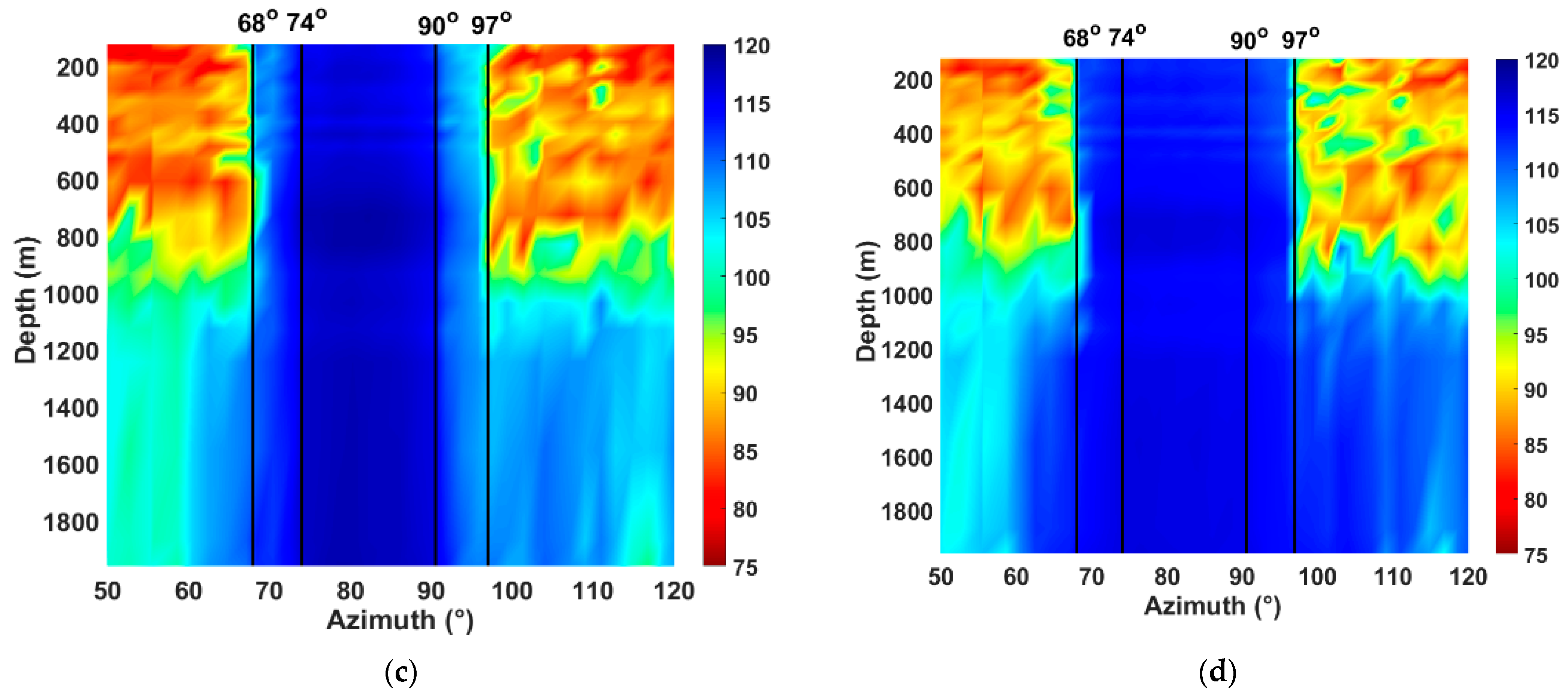
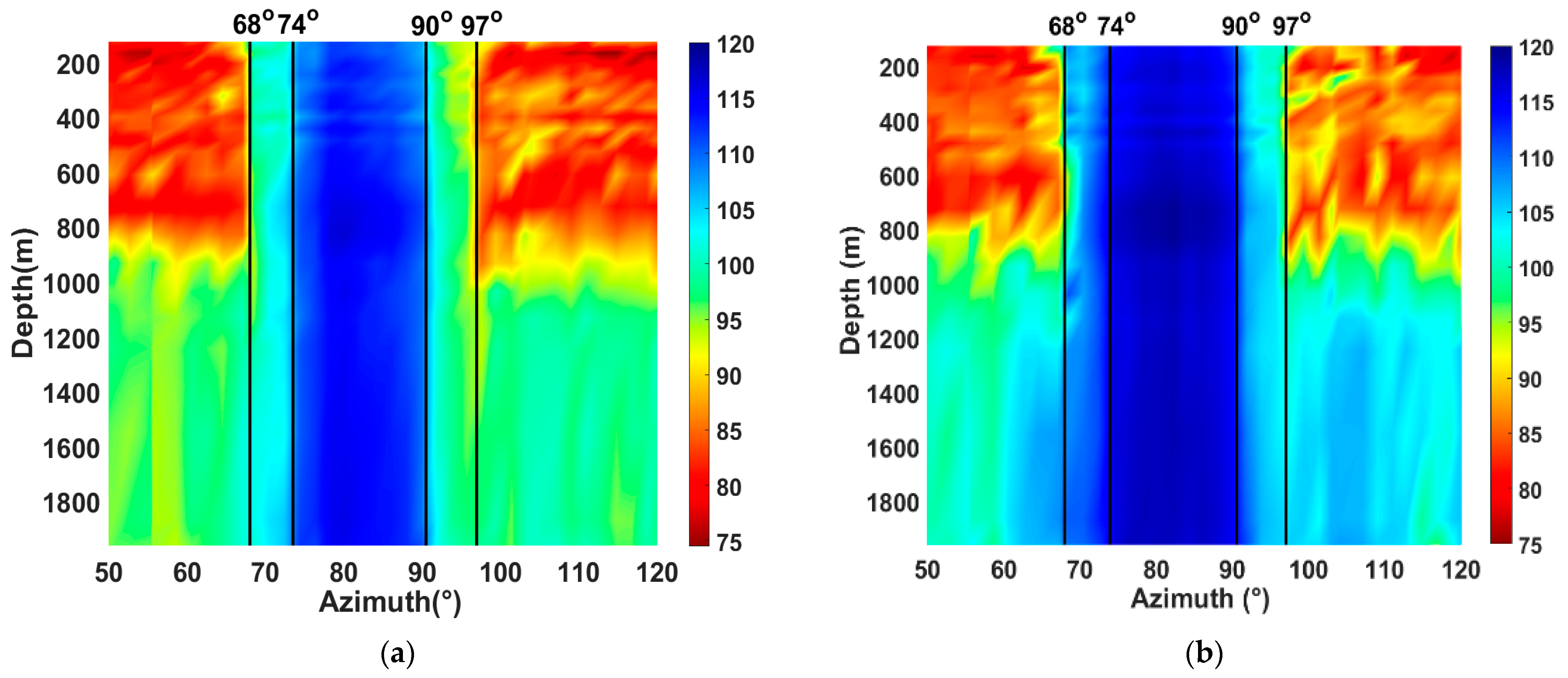
Figure 6 shows the experimental TLs varying with the azimuth and depth in the O2T3T3 track, where the azimuth angle ranged from 50° to 120° and the central frequencies were 300 Hz, 1000 Hz, 1500 Hz, and 3000 Hz. It can be observed from Figure 6a that the high sound intensity zone was formed in the range of 50–68° and 97–120°, and the structure of the convergence zone was destroyed in the range of 68–97°. In the range of 74–90°, the seamount had a more obvious influence on sound propagation, which caused the acoustic shadow zone behind the seamount, and the horizontal refraction zone with obvious boundaries between the high sound intensity zone and shadow zone appeared in the range of 68–74° and 90–97°. It can be seen from Figure 6a that the TLs in the shadow zone were 10–15 dB larger than those in the horizontal refraction zone and 30–40 dB larger than the TLs in the high sound intensity zone. In Figure 6b–d, it can be found that the horizontal refraction zone decreased gradually as the frequency increased because of the absorption of sea water and the sea bottom. It was difficult to observe obvious 3D effect phenomena when the frequency increased. In order to facilitate the subsequent analysis of the 3D effect phenomena, the low frequency (300 Hz) was selected as the analysis object in this paper.

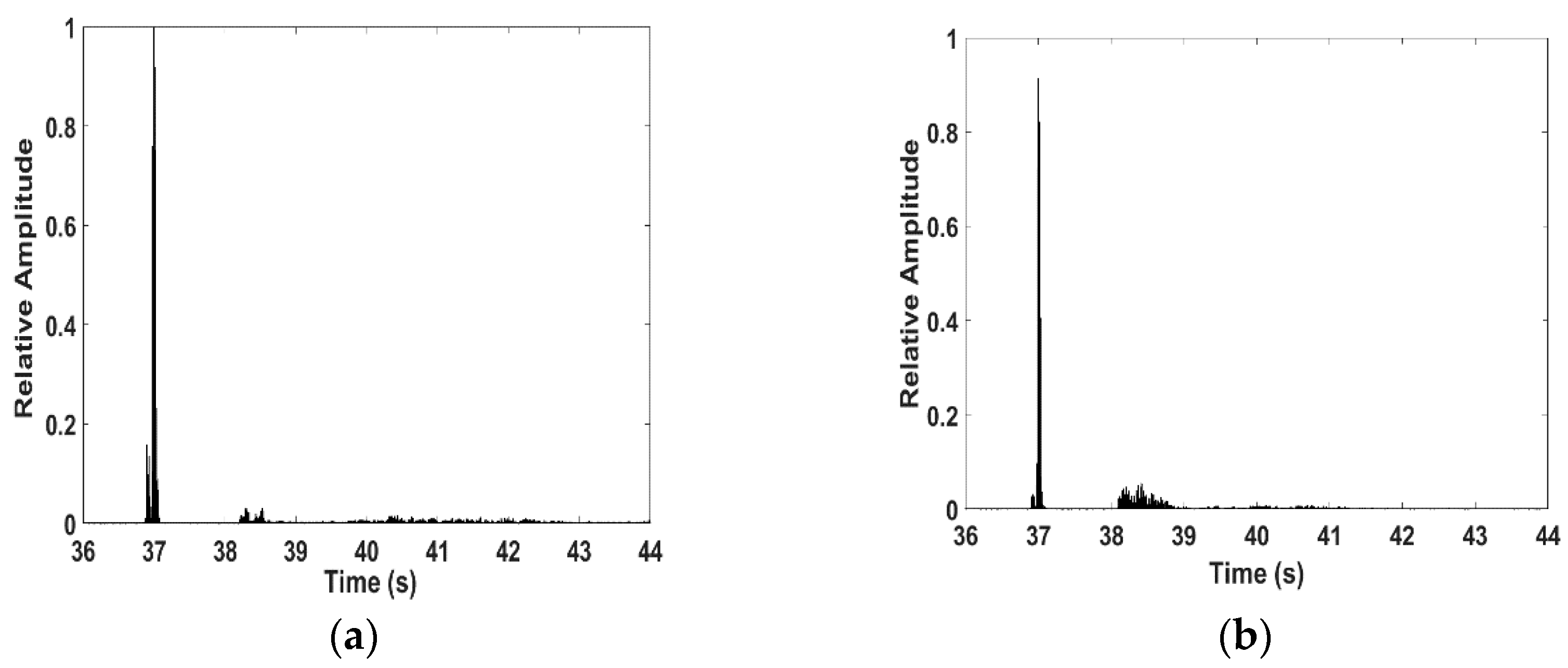
Figure 7 gives the experimental sound signals in the time domain received by the hydrophone when the explosive sources were located at 54.82°, 64.66°, 66.65°, and 70.62° in the O2T3T3 track, and the center frequency was 300 Hz with a bandwidth of a 1/3 octave band, where the receiver depth was 525 m. The Y-axis represents the relative amplitudes of the sound signals, and the signal of 54.82° was selected as a benchmark for normalization processing because the sound waves propagated in the flat bottom. The effect of the seamount in different directions on the sound signals in the time domain could be observed intuitively by comparing the relative amplitudes of the signals. It could be found that the influence was increasingly significant for the signals as the height of the seamount increased, and the relative amplitudes of the sound signals and the arrival time interval between the direct wave and the pulse arriving at the receiver after the reflections decreased gradually.

3. Explanation of the 3D Effects

In order to study the 3D effects of a seamount on sound propagation, the BELLHOP N×2D and 3D ray models [10] were used to calculate and analyze the sound field of the seamount. According to the principle of reciprocity [11], the positions of the source and receiver are exchanged in the calculation. In 2014, the sediments of the seabed surface were sampled in an experiment of sound propagation which was conducted in this area. The results of the sample analysis are shown in the

Table 1. The results of the seabed sediment samples.

Sound Speed (m/s)	Density (g/cm3)	Porosity (%)	Grain Size (mm)	Sediment Type
1508–1695	1.21–1.65	62.60–85.55	0.0046–0.0287	Clay-silty

, and the results are discrete. The sediment type of the seabed surface was clay-silty. Two layers of the fluid bottom model were established with a sediment thickness of 5 m, a sediment sound speed of 1565 m/s, a sediment density of 1.6 g/cm³, a sediment attenuation coefficient of 0.09 dB/m, a basement sound speed of 1650 m/s, a basement density of 1.8 g/cm³, and a basement attenuation coefficient of $0.4\times {(f/1000)}^{0.9}$ dB/$\lambda$, where $f$ is expressed in kHz [8].

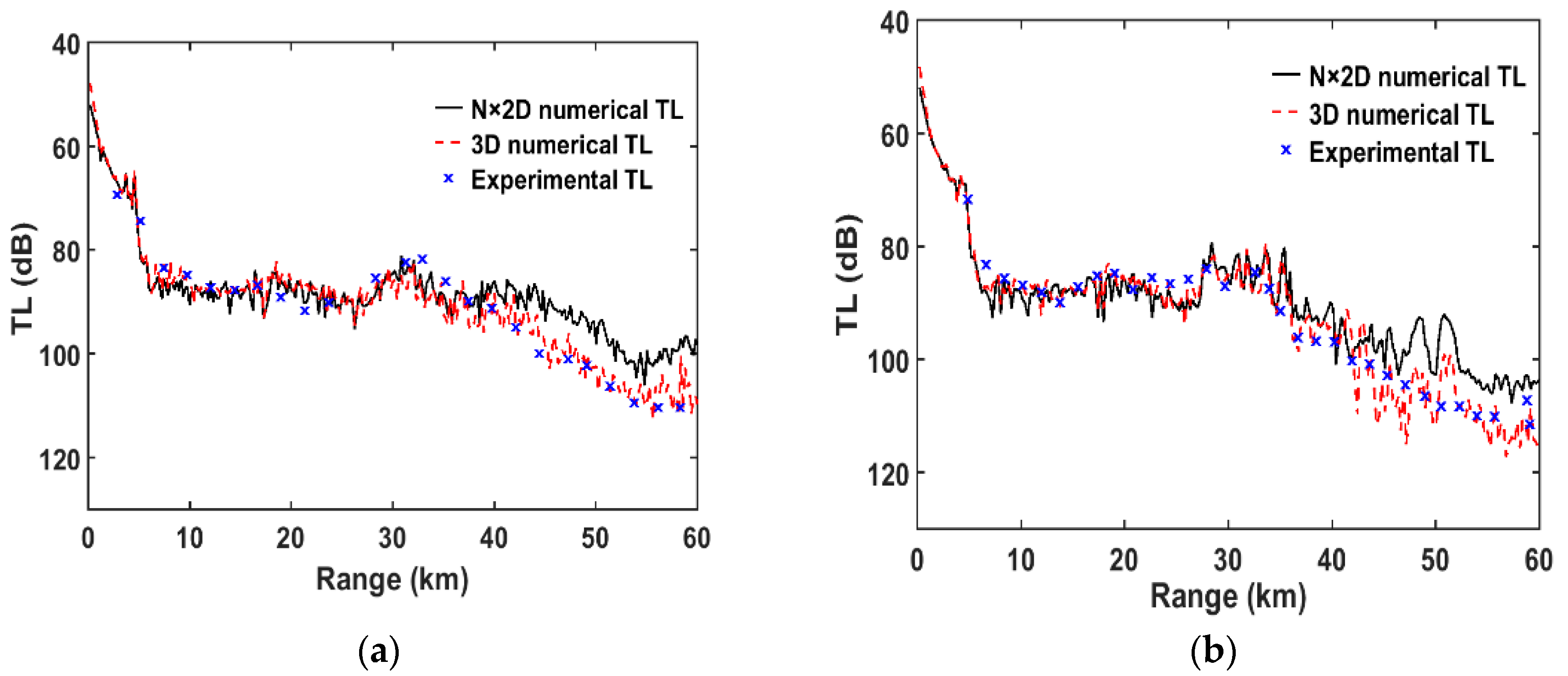
The comparison of the numerical and experimental TLs calculated by the N×2D and 3D models along the O2T9 and O2T2 tracks is given in Figure 8, where the central frequency is 300 Hz and the receiver depth is 525 m. It is of note in Figure 8a that the TLs calculated by the 3D model were consistent with the experimental TLs in the O2T9 track. At a range of 0–38 km, the N×2D and 3D model TL results were similar, which indicates that the 3D effect was not obvious in this area. However, in the rear of the seamount on the O2T9 track, the TLs calculated by the N×2D model were about 10 dB smaller than the 3D model results, which represents that the 3D effect of the seamount had impacts on sound propagation in this area. A similar conclusion can be observed for the O2T2 track in Figure 8b.

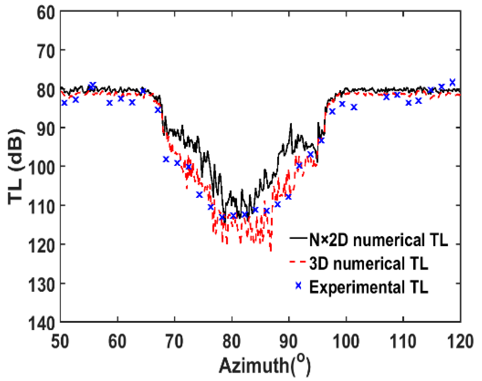
Figure 9 shows the comparison of the numerical and experimental TLs along the O2T3T3 track in the range of 50–120°, where the central frequency is 300 Hz and the receiver depth is 525 m. It can be found that the TLs calculated by the 3D model basically matched the experimental results, but the TLs calculated by the N×2D model were about 5–10 dB smaller than the 3D model results, which represents that the 3D effect of the seamount had an impact on the horizontal refraction zone and shadow zone behind the seamount.

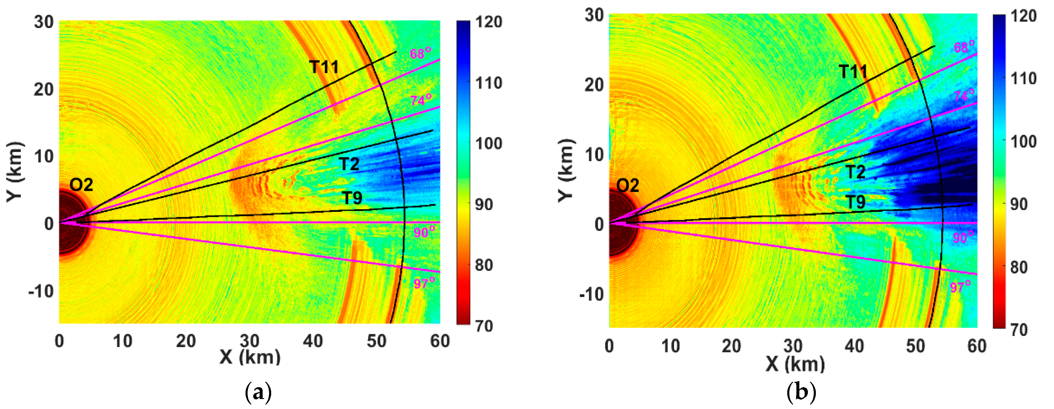
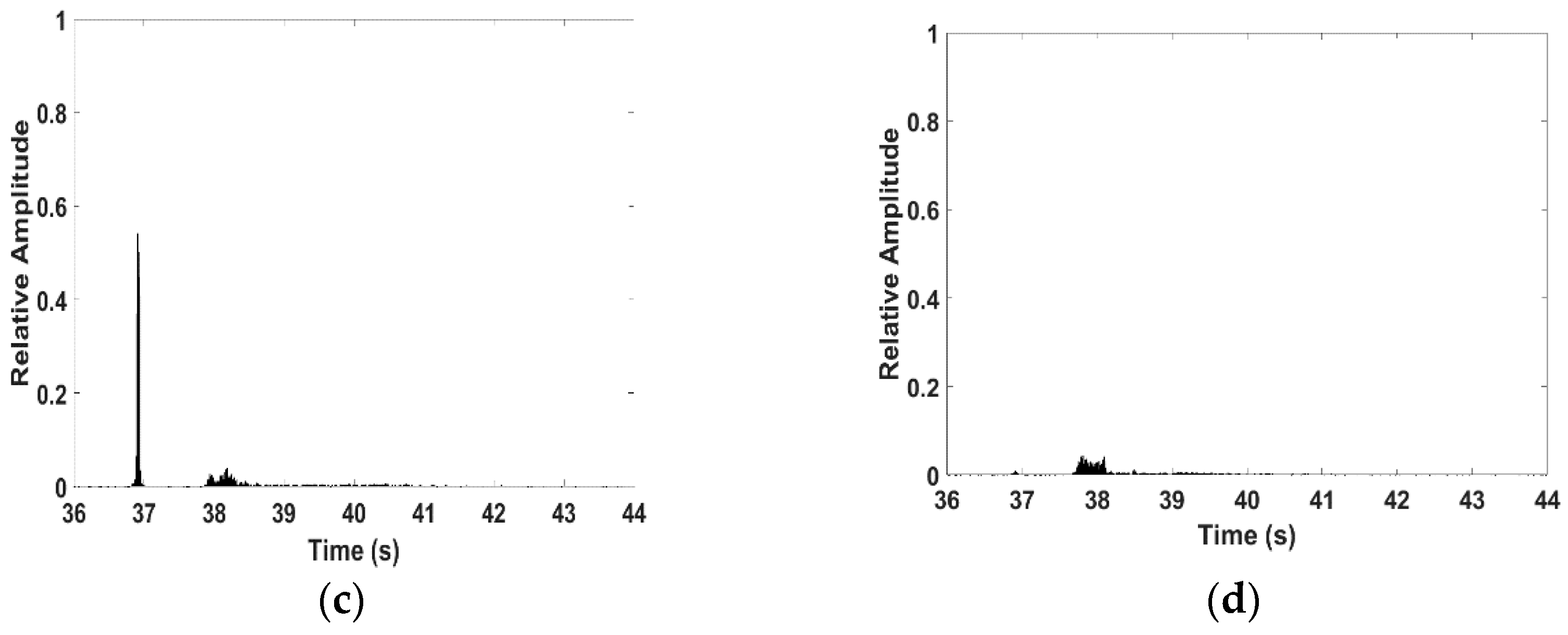
The numerical TLs obtained by the N×2D and 3D models are illustrated in Figure 10a,b, where the central frequency is 300 Hz and the receiver depth is 525 m. It can be seen from Figure 10 that the convergent zone structures were destroyed by the direct blockage of the seamount, which led to the increase in the TLs. Shadow zones and horizontal refraction zones which existed between the shadow zone and high sound intensity area appeared behind the seamount. The difference between the TLs in the shadow zone and the horizontal refraction zone was about 10–15 dB. The numerical sound field structure behind the seamount obtained by the 3D model was different from the N×2D model’s result, in which the width of the shadow zone calculated by the 3D model was wider than that calculated for the N×2D model, and the width of the horizontal refraction zone from the 3D model was narrower than the N×2D model’s result, while the TLs were similar at other positions.

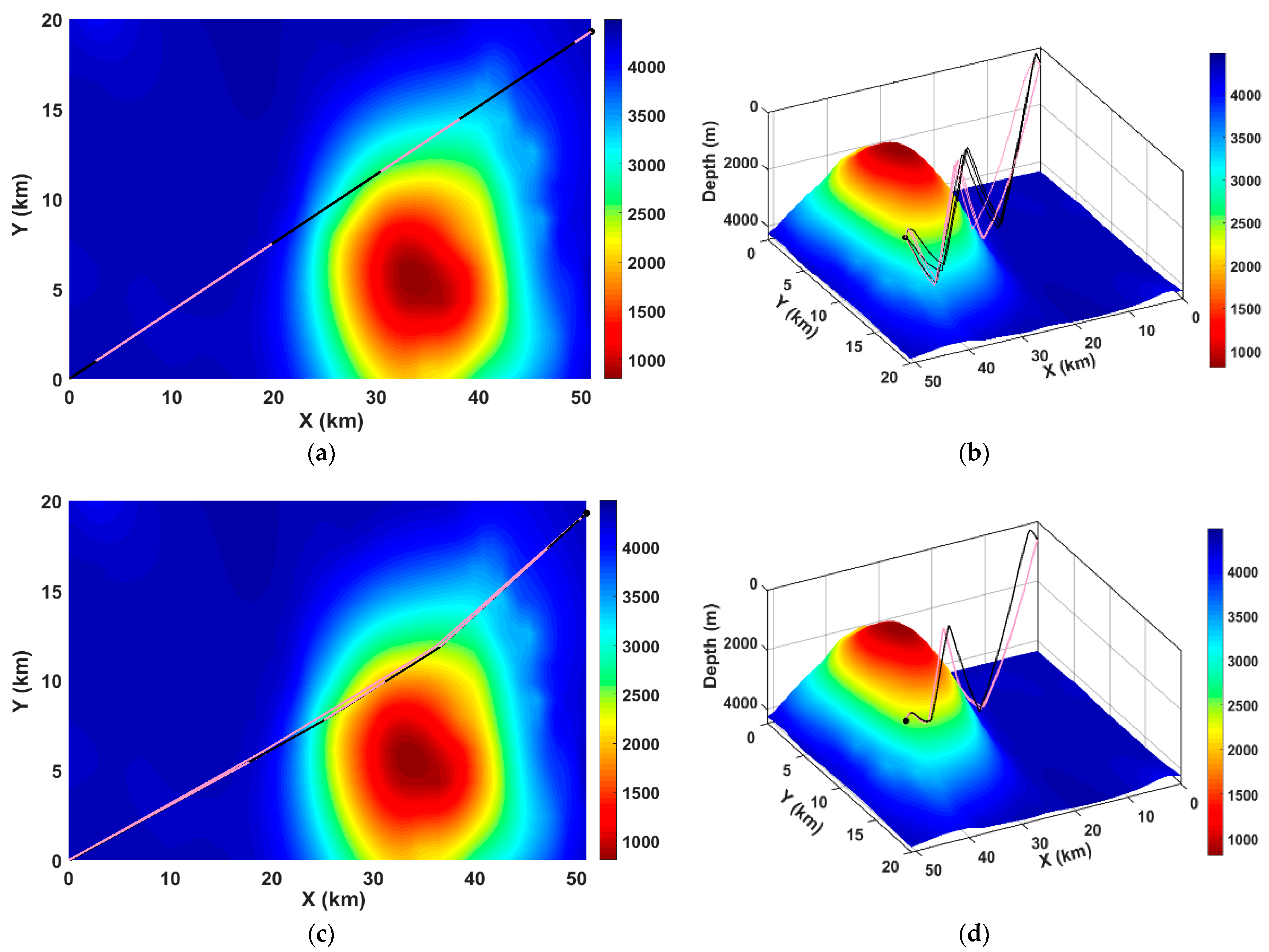
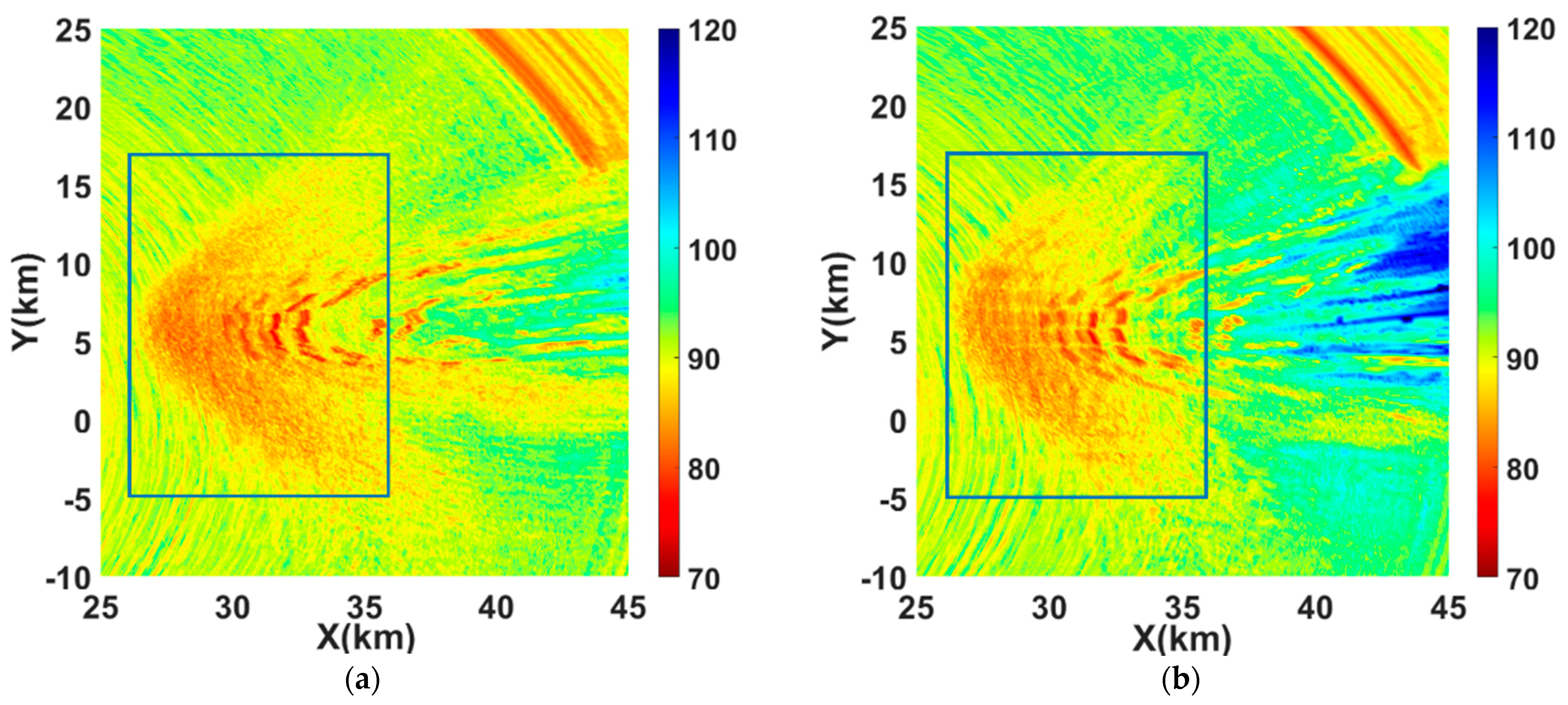
Figure 11 shows the eigenrays calculated by the N×2D and 3D models when the sound source was located in the refraction zone, where the sound source was located at X = 51 km, Y = 19 km, Z = 200 m and the receiver was located at X = 0 km, Y = 0 km, Z = 525 m. It can be seen from Figure 11a,b that the eigenrays obtained from the N×2D model propagated in a straight direction. There were no direct waves reaching the receiver due to the blockage of the seamount, and there were only eigenrays which interacted with the seamount once or twice before reaching the receiver. Figure 11c,d shows the eigenrays obtained from the 3D model, reaching the receiver after horizontal refraction of the seamount. The eigenrays also consisted of which interacted with the seamount once or twice, but the eigenrays obtained from the 3D model are lesser than those obtained from the N×2D model. Therefore, the sound energy calculated by the N×2D model would be greater than the results of the 3D model, which could explain the phenomenon of the TL results calculated by the N×2D model being about 10 dB larger than the 3D model results in the horizontal refraction zone. The 3D effect of the seamount had a certain influence on the sound field in the horizontal refraction zone.

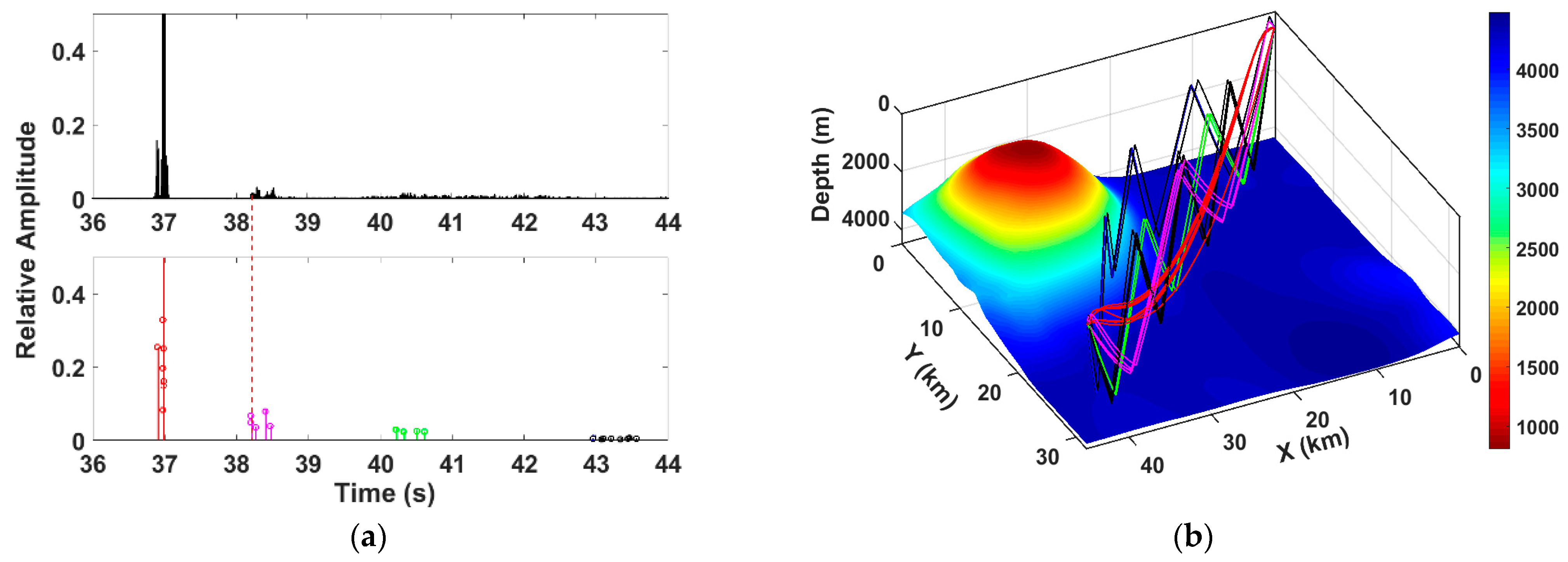
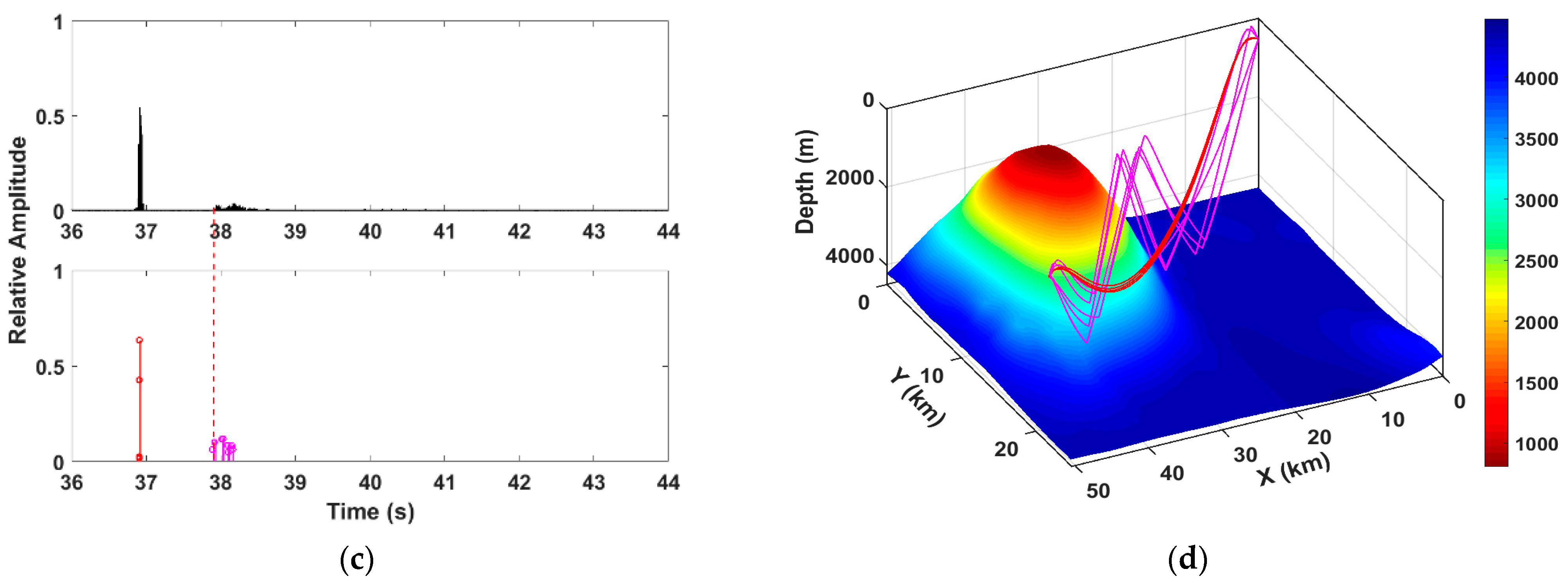
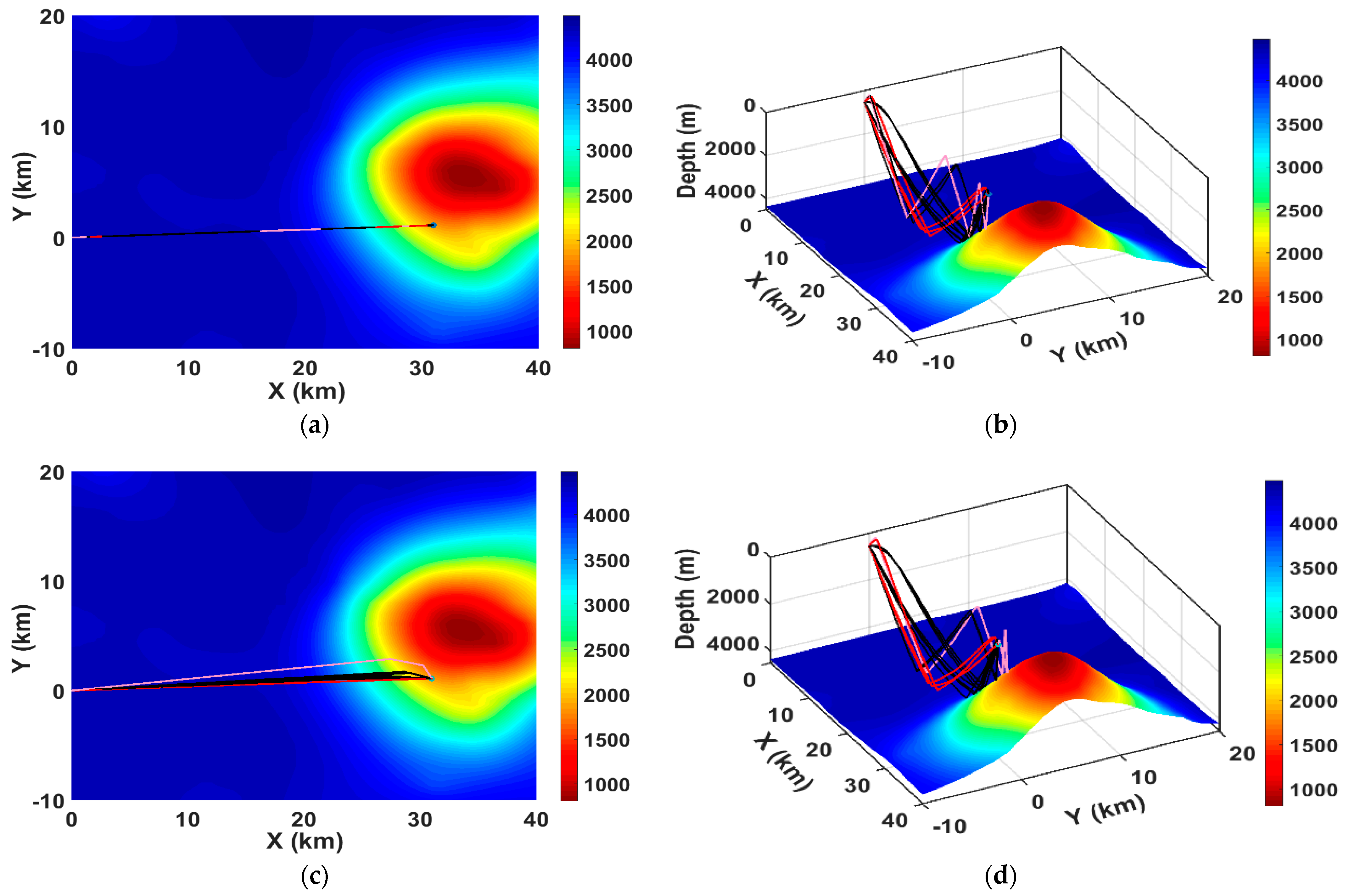
Next, the horizontal refraction effects of the seamount on the arrival structures were investigated. Figure 12 shows the arrival structures and the eigenrays obtained by the 3D model at an azimuth angle of 54.82° and 66.65°, where the source depth was 200 m and the receiver depth was 525 m. In Figure 12a,c, the above images give the experimental signals, and the images below give the numerical arrival structure results. The eigenrays obtained by the 3D model are shown in Figure 12b,d. It can be found that the arrival structures calculated by the 3D model were consistent with the experimental signals. The wave paths after reflection would be gradually shortened as the height of the seamount increased, which made the arrival time interval between the direct wave and the pulse arriving after reflections decrease gradually.

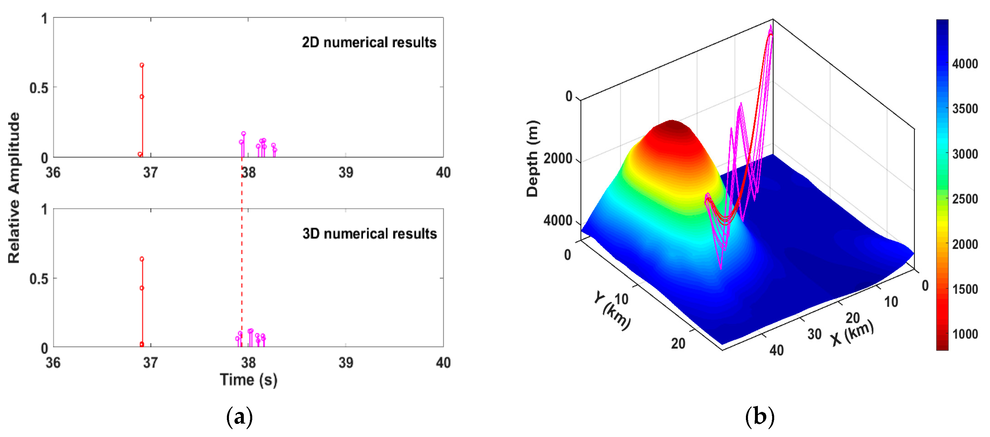
In terms of the sound source at 66.65°, the comparison of the arrival structure obtained from the 2D and 3D ray models and 2D results of the eigenrays are shown in Figure 13, where the source and the receiver depth are 200 m and 525 m, respectively. It can be found that the propagation path of the sound rays would be shortened due to the refraction effect of the seamount, which caused some rays obtained from the 3D model to reach the receiver about 0.05 s earlier than the sound rays of the 2D model.

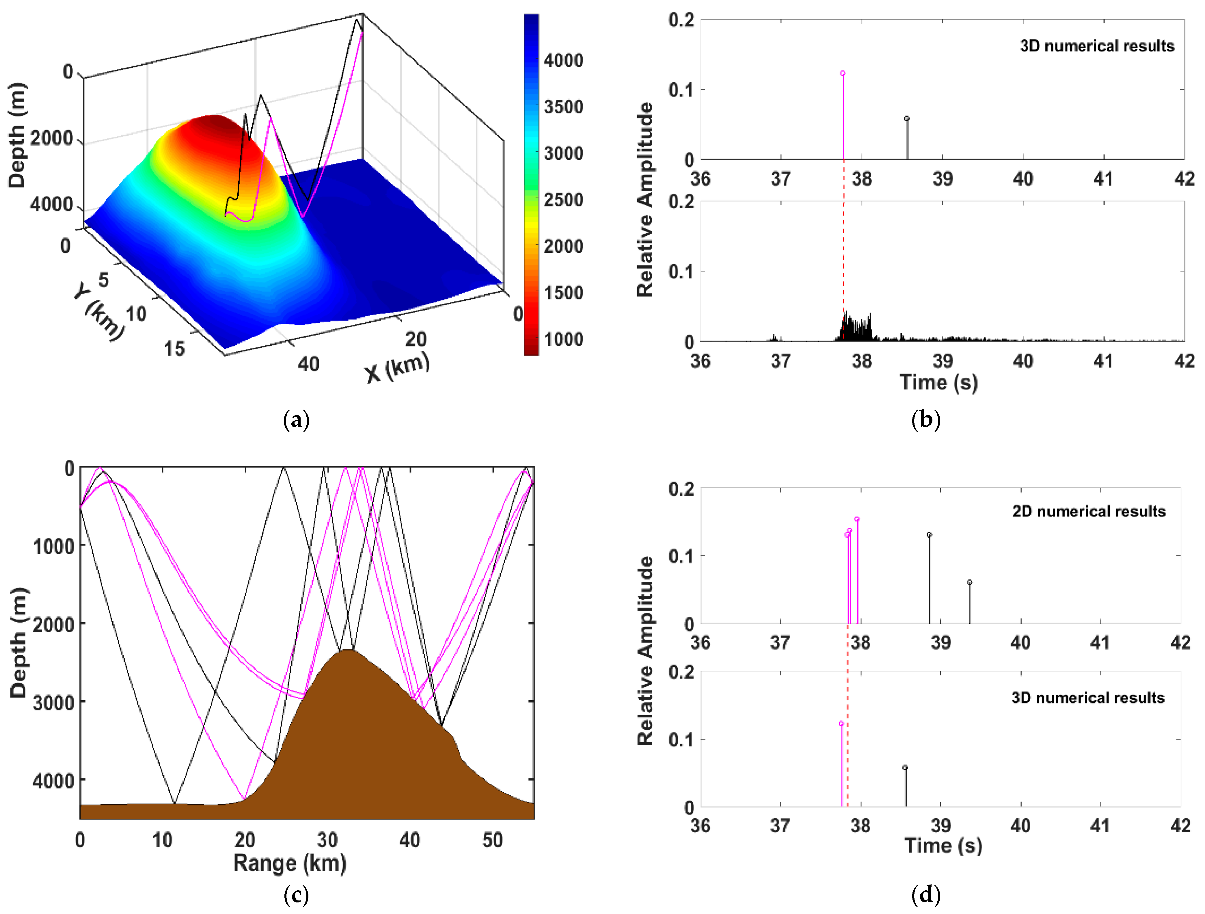
Figure 14 shows the 3D and 2D results of the eigenrays and the comparison of the 2D and 3D arrival structures when the is source located at 70.62°. It can be seen from Figure 14 that the arrival structures obtained by the 3D model were less than those obtained by the 2D model. Figure 14b gives the comparison of the 3D arrival structures and the experimental signal, and it can be found that the simulated arrival times were consistent with the experimental results. Moreover, the arrival structures of the experimental signal were greater than those of the numerical results, which may have been due to the surface of the seamount not being smooth and there being other arrival structures. In Figure 14d, the eigenrays after horizontal reflection arrived at the receiver earlier than those obtained from the two-dimensional (2D) model within the horizontal refraction zone behind the seamount. This means that the horizontal reflection effect of the seamount would shorten the sound propagation paths.

Finally, the 3D effect of the seamount on the reflection zone of the seamount was studied. Figure 15a,b shows the numerical TL results obtained from the N×2D and 3D models in the reflection zone of the seamount. It is obvious that the reflection zone of the seamount within the range of 26–36 km seemed like an “arch” type, which was the shape of the reflection zone of the seamount, and the distances between the reflection area and the receiver were different. It can be seen from the comparison of the N×2D and 3D numerical TL results that the horizontal refraction of sound waves had little effect on the TLs in the reflection zone of the seamount.

To give a theoretical explanation, Figure 16 shows the 2D and 3D eigenray results of the acoustic reflection zone. It can be found that the horizontal refraction effect of the eigenrays interacting with the seamount once was little, and the wave paths could be approximated as propagating along a straight direction. Aside from that, the compositions of the 2D and 3D eigenrays were basically same, which proved that the horizontal refraction of sound waves had little effect on the TLs in the reflection zone of the seamount.

In the end, the 2D numerical TL results of different tracks are shown in Figure 17a,b with a source depth of 200 m, receiver depth of 525 m, and central frequency of 300 Hz. It can be seen that the ranges of the reflection areas of the seamount were different because the slopes, heights, and distances of the seamount from the receiver had differences. In the direction of the O2T2 track, the distance between the seamount and the receiver was smaller than that in the direction of the O2T9 track, and the slope of the seamount was steeper than that in the direction of the O2T9 track, which caused the reflection zone of the O2T2 track to be about 1.5 km closer than that in the direction of the O2T9 track. Therefore, the difference in the cross-section of the conical seamount made the shape of the reflection zone seem like an “arch” type.

4. Conclusions

An experiment was conducted to investigate the effects of seamounts on sound propagation in deep water. The effects of seamount on sound propagation in deep water were investigated. Three-dimensional propagation phenomena due to the seamounts were observed. The propagation mechanism was analyzed by using the ray theory. The 3D effects of the seamounts had obvious impacts on the sound field within a certain angle range behind the seamount. Some of the sound beams could not reach the receiver because of the horizontal refraction effects. The rays obtained from the 3D model arrived at the receiver earlier than those obtained from the 2D model, which means that the horizontal reflection effect of the seamount would shorten the sound propagation paths, and the arrival structures obtained by the 3D model were lesser than those in the 2D model simulation results when the source was located in the horizontal refraction zone. Finally, it can be found that the horizontal refraction of sound waves had little effect on the TLs in the reflection zone of the seamount. The shape of the TLs in the reflection zone of the conical seamount seemed like an “arch” type, which was due to the different cross-sections of the seamounts causing changes in the horizontal position of the reflection area in different directions.