Double-Loop Sliding Mode Controller with An Ocean Current Observer for the Trajectory Tracking of ROV

Abstract

To solve the trajectory tracking problem of insufficient response and the large tracking error of remotely operated vehicles (ROVs) under the interference of large ocean currents, this paper proposes a double-loop sliding mode controller with an ocean current observer. The designed controller consisted of an outer-loop controller (the position controller) and an inner-loop controller (the velocity controller): the outer controller was designed by the position error, and a reference velocity was created for the inner loop to achieve accurate positioning and attitude tracking. The reference control input was treated as a new target to design the inner-loop controller, enabling the ROV to achieve accurate reference velocity tracking. Based on the theoretical idea of active disturbance rejection control, a kinematic equation-based ocean current observer was designed to estimate and compensate for large unknown currents to ensure accurate trajectory tracking performance under large currents. The simulation results proved that the double-loop sliding-mode control scheme with an ocean current observer always showed good tracking performance, demonstrating the excellent control performance and high robustness of the scheme. Compared with the high-complexity control schemes such as neural network-based PID control or fuzzy sliding mode control, it effectively improves the robustness to ocean current disturbances without increasing the computational effort excessively, and is more practical in ROV systems with limited computational power.

1. Introduction

With the explore and exploit process of marine resources, remote operation vehicles (ROVs) play an important role in many marine production activities. ROVs are most commonly used for the inspection of underwater structures, pollutant detection and localization, marine resource exploration, oceanographic mapping [1,2], etc. In practical applications, light-weight-observation ROVs have become a powerful tool for offshore observation due to their advantages of low-cost manufacture, reliable performance, and flexible usage. Unlike the deep-sea environment, currents and tides are the dominant environmental factors in coastal oceans. Therefore, observation-type ROVs for coastal ocean tasks should be capable of bearing the interference of ocean current. In recent years, relevant scholars [3,4] have conducted a series of effective research attempts on ROV control under the interference of ocean currents. In most regions, the average current speed in offshore operation areas is about 2.0 knots, and the extreme current speed even reaches more than 6.0 knots [5]. Therefore, it is necessary to develop the trajectory tracking controller of ROVs according to the conditions of ocean currents.

In order to eliminate current interference, many outstanding control methods have been adapted for ROVs’ control, such as PID control [6,7], adaptive control [8,9,10], backstep control [11,12], and sliding mode control (SMC) [13,14,15,16]. In addition, fuzzy logic control [13,17,18] and neural network control [7,19,20] are often used in combination with other control methods. Among the mentioned control methods, SMC is increasingly used for the trajectory tracking control of ROVs under complex sea conditions because of its robustness to parameter changes and good suppression of external disturbances. However, traditional SMC faces the significant problem of chatter. Researchers often try to use a combination of different control methods when applying sliding control. Xu et al. [16] proposed a novel adaptive dynamical sliding mode control model, which combines backstepping control with traditional SMC. This model enhances the robustness of ROVs under the conditions of systematical uncertainty and environmental disturbances. Yan and Yu [15] designed a finite-time disturbance observer to observe the unknown time-varying disturbances for autonomous underwater vehicles (AUVs), and the scheme attempts to account for quantization effects in the AUV control design. Valdovinos et al. [14] proposed a second-order sliding mode control in combination with a backpropagation neural network (BP-NN) control scheme for ROVs to deal with external disturbances. Vu et al. [21] designed a position-keeping control scheme based on SMC theory and a thrust distribution algorithm with the lowest energy consumption to effectively ensure the stability and better performance of ROVs. Methods such as the adaptive sliding mode scheme [22] and adaptive fast terminal sliding mode scheme [23] for nonlinear systems also greatly expand the application scenarios of the sliding mode control and show the scientific potential and application value of SMC. Considering the actual operating environment of ROVs, ocean currents are often random and difficult to model [24]. Therefore, most current controllers for ROVs are based on the assumptions that the currents are nonspinning and constant or slowly changing [25,26]. Based on this assumption, dual-loop control structures and active disturbance rejection control may be solutions worth considering.

The active disturbance rejection control (ADRC) presented by Han [27] has shown its unique value in suppressing interference by considering the disturbance of large ocean currents as an external disturbance to be suppressed. Habib and Zhu [28] presented a generalized extended-state observer (ESO) and harmonic ESO for path tracking control of ROVs to improve ADRC performance. Two path-tracking controllers were designed to ensure an outstanding performance under significant fast-varying disturbances caused by waves and sea currents. A robust control method based on lumped perturbation observer was proposed by Thanh et al. [29] for a system with matched and unmatched uncertainties. The scheme applies the multiple surfaces to approximate the unknown lumped perturbations simultaneously influencing a nonlinear system. This demonstrates the great significance of state observers to improve the control performance of the system. Zhang et al. [3] presented a position-tracking controller and a current observer by using the backstepping technique in the presence of unknown ocean currents, and the final controlled system was proved to be globally K-exponentially stable by stability criteria for the cascade system. Although the study was limited to non-time-varying currents, it also showed that the ADRC scheme is an effective way to consider for ROV control under ocean currents.

In the research of the interference suppression of complex control systems, the double-loop control structure has been successfully used in permanent-magnet synchronous motors [30], piezoelectric-actuated inertial stick-slip devices [31], automotive electronic throttle control [32], etc. In recent years, there have been many attempts in the field of ocean engineering. Mu et al. [33,34] proposed an improved double PD control method for typical nonlinear and large-time-delay systems (profiling float). The low-power control strategy for the floating process and the real-time prediction of position were proposed, which resulted in favorable robustness and stability for nonlinear time-varying floating systems. Qiao and Zhang [35] proposed two adaptive integral terminal SMC schemes based on integral terminal sliding mode (ITSM) and fast ITSM (FITSM). An adaptive mechanism was introduced to estimate the uncertainty parameters of the lumped system, which consists of dynamic uncertainties and time-varying external disturbances. Huang and Yang [36] applied a double-loop SMC to work-class ROVs’ trajectory tracking. Singular perturbation theory and the concept of speed variation were used to separate the ROV’s state into two systems with different rates. Considering the practical situations where systematic parametric uncertainties and external disturbances exist, Yan et al. [37] presented an adaptive integral SMC for underactuated AUVs. Moreover, a novel direct adaptive neural network controller combined with a conditional integrator was presented, which provides the robustness and adaptation for the vehicle. The aforementioned studies showed that, for the control of nonlinear and complex systems in the field of offshore engineering, the double-loop control structure exhibited strong robustness against external disturbances through the natural advantage of hierarchical control.

Effective control of ROVs under disturbing conditions of large ocean currents is a challenging task. SMC has become a hot topic in ROV trajectory tracking control due to its robustness and excellent control performance. The essence of trajectory tracking is to achieve perfect control of position and velocity, but traditional sliding mode control tends to consider only position matching, so the dual-loop control structure has become our target solution. To achieve the effective control of ROV systems, Rojsiraphisal and Vu [38] et al. proposed the idea of combining the state observer and terminal sliding mode control, which greatly inspired the present scheme. We tried to construct a double-loop control structure for the trajectory tracking control of ROVs. Furthermore, the role of ocean currents with the ROV system is often complex and difficult to define clearly. A kinematic equation-based ocean current observer was designed to estimate and compensate for large unknown currents to ensure accurate trajectory tracking performance under large currents. Expectedly, the response difference between the velocity loop and the position loop helped to improve trajectory tracking performance and shorten the controller response time.

The rest of this paper is organized as follows: Section 2 introduces and describes a simplified mathematical model of the underwater robot and an ocean current model. Section 3 introduces the structure of a double-loop SMC scheme with an ocean current observer module. In Section 4, numerical simulation experiments are conducted based on the self-developed ROV model for submarine cable detection. The performance analysis and robustness comparison of different control schemes are carried out for the two trajectory tasks under different ocean currents. Finally, Section 5 summarizes the conclusions of the paper.

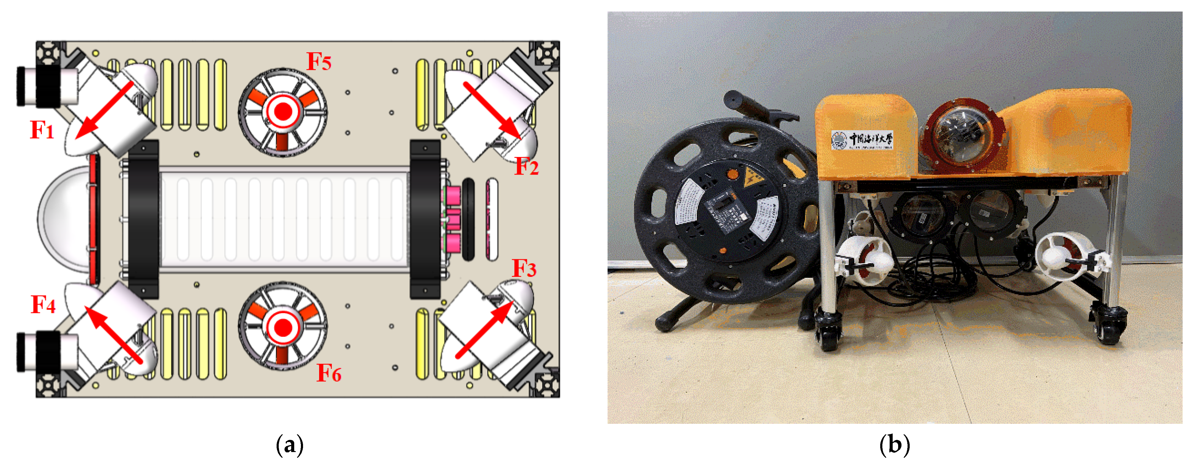
2. Hydrodynamic Model and Simplification

2.1. Assumptions

To accurately describe the motion of ROVs in 3D space, we usually define two coordinate systems, as shown in Figure 1. The positive direction of the inertial frame is specified as the main heading of ROVs. The origin of the body-fixed frame coincides with the center of gravity of the ROV’s body structure. Both are defined as right-handed Cartesian coordinate frames. The actual motion model of ROVs is highly nonlinear and difficult to model, so we have made some simplifications with reference to the convention. These simplifications are as follows:

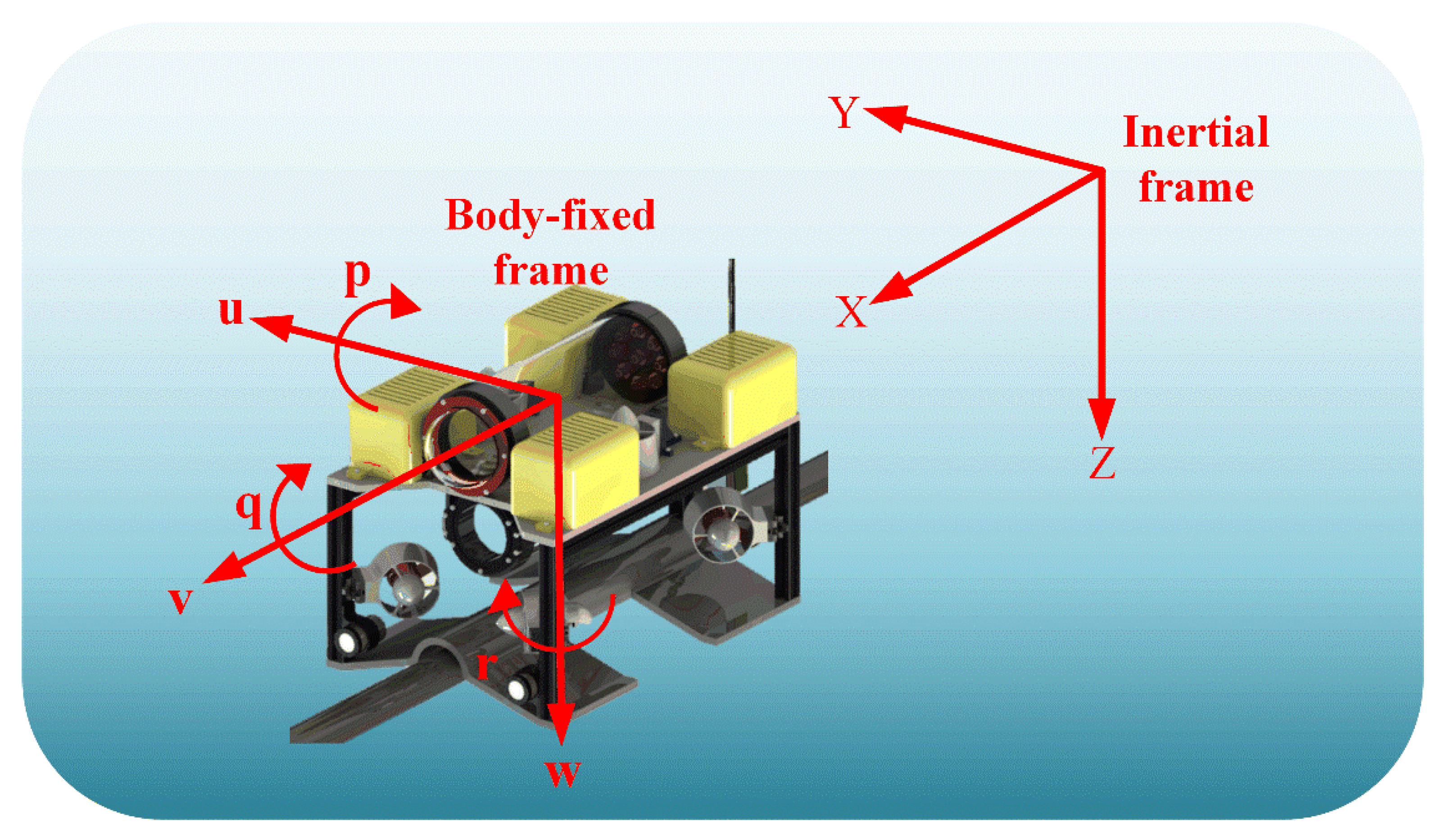
• ROVs are retained in only four degrees of freedom: sway, surge, heave, and yaw;
• The floating center of ROVs is on the same line as the center of mass;
• The nonlinear response of the thruster is not considered;
• The unmentioned disturbances are not considered in the dynamical equations.

2.2. Kinematic Model

The position and orientations with respect to the inertial frame are denoted by $\eta ={\left[x,y,z,\phi ,\theta ,\psi \right]}^T$. The linear velocity and the angular velocity with respect to the body-fixed frame are represented by $v={\left[\mathrm{u},v,w,p,q,r\right]}^T$. By using a Jacobian transformation matrix, the relationship between the derivatives of the linear and angular velocities in the inertial coordinate frame and those in the body-fixed frame can be expressed as:

$$\dot{\eta }=J\left(\eta \right)v=\left[\begin{array}{cc}{J}_1\left(\eta \right)& 0\\ 0& J_2\left(\eta \right)\end{array}\right]\nu$$

(1)

where

$$J_1\left(\eta \right)=\left[\begin{array}{ccc}\mathrm{c}\gamma \mathrm{c}\theta & \mathrm{c}\gamma \mathrm{s}\theta \mathrm{s}\phi -\mathrm{s}\gamma \mathrm{c}\phi & \mathrm{c}\gamma \mathrm{s}\theta \mathrm{c}\phi +\mathrm{s}\gamma \mathrm{s}\phi \\ \mathrm{s}\gamma \mathrm{c}\theta & \mathrm{s}\gamma \mathrm{s}\theta \mathrm{s}\phi +\mathrm{c}\gamma \mathrm{c}\phi & \mathrm{s}\gamma \mathrm{s}\theta \mathrm{c}\phi -\mathrm{c}\gamma \mathrm{s}\phi \\ -\mathrm{s}\theta & \mathrm{c}\theta \mathrm{s}\phi & \mathrm{c}\theta \mathrm{c}\phi \end{array}\right]$$

(2)

$$J_2\left(\eta \right)=\left[\begin{array}{ccc}1& \frac{\mathrm{s}\phi \mathrm{s}\theta }{\mathrm{c}\theta }& \frac{\mathrm{c}\phi \mathrm{s}\theta }{\mathrm{c}\theta }\\ 0& \mathrm{c}\phi & -\mathrm{s}\phi \\ 0& \frac{\mathrm{s}\phi }{\mathrm{c}\theta }& \frac{\mathrm{c}\phi }{\mathrm{c}\theta }\end{array}\right]$$

(3)

where the symbols s and c represent trigonometric functions $s=\sin (\cdot )$ and $c=\cos (\cdot )$, respectively. The ROVs are usually capable of self-equilibration in the XZ and YZ planes, due to a strong buoyancy recovery torque. Therefore, the assumption that $\varphi =\theta =0$ is satisfied. Hence, the 6 degree-of-freedom equation (Equation (1)) for ROVs can be simplified to a 4-DOF model.

$$\left[\begin{array}{c}\dot{x}\\ \dot{y}\\ \dot{z}\\ \dot{\psi }\end{array}\right]=\left[\begin{array}{cccc}\mathrm{c}\psi & -\mathrm{s}\psi & 0& 0\\ \mathrm{s}\psi & \mathrm{c}\psi & 0& 0\\ 0& 0& 1& 0\\ 0& 0& 0& 1\end{array}\right]\left[\begin{array}{c}u\\ v\\ w\\ r\end{array}\right]$$

(4)

2.3. Hydrodynamic Model

The motion of an ROV can be considered as the general motion of a rigid body in a fluid subjected to gravity and hydrodynamic forces. The kinetic equation of an ROV in an inertial coordinate system [24] can be expressed by Equation (5).

$$M\dot{v}+C\left(v\right)v+D\left(v\right)v+g\left(\eta \right)=\tau$$

(5)

where rigid mass and added mass form the mass matrix denoted by $M\in R^{4\times 4}$, $C\left(v\right)\in R^{4\times 4}$ is the Coriolis and centripetal force matrix, $D\left(v\right)\in R^{4\times 4}$ is the damping matrix, and $g\left(\eta \right)\in R^{4\times 4}$ is the restoring force matrix. $\tau \in R^{4\times 4}$ is the control force and moment vector.

The mass matrix M contains two parts: the mass matrix of the rigid body M_RB and the added mass matrix M_A. Thus, it can be simplified as:

$$M=\left[\begin{array}{cccc}m-X_{\dot{u}}& 0& 0& 0\\ 0& m-Y_{\dot{v}}& 0& 0\\ 0& 0& m-Z_{\dot{w}}& 0\\ 0& 0& 0& I_Z-N_{\dot{r}}\end{array}\right]$$

(6)

where m represents the mass of the ROV, and the ROV moment of inertia about the Z-axis is represented by $I_z$. $X_{\dot{u}},\begin{array}{c}\end{array}{Y}_{\dot{v}},\begin{array}{c}\end{array}{Z}_{\dot{w}}$, and $N_{\dot{r}}$ represent the corresponding added mass and additional inertia.

The Coriolis and centripetal force matrices in the motion equations can be suitably simplified to meet the needs of numerical simulations. Considering the model assumptions of ROVs and the lower cruising speed, it can be obtained that,

$$C\left(v\right)=\left[\begin{array}{cccc}0& 0& 0& -\left(m-Y_{\dot{v}}\right)v\\ 0& 0& 0& \left(m-X_{\dot{u}}\right)u\\ 0& 0& 0& 0\\ \left(m-Y_{\dot{v}}\right)v& -\left(m-X_{\dot{u}}\right)u& 0& 0\end{array}\right]$$

(7)

The main reasons for the appearance of the damping term are: potential flow damping due to motion in the fluid; frictional damping due to the relative motion of the ROV surface and the fluid; wave-making damping caused by generating waves; and vortex shedding damping due to the vortex generated when the fluid flows through the ROV. If the underwater robot has three symmetrical surfaces, a linear approximation can be made so that the second-order terms and above can be neglected. Therefore, the calculation of the damping term can be summarized as linear damping and nonlinear damping, where the nonlinear component will account for a larger percentage. The following equation is expressed as:

$$D\left(v\right)=-\left[\begin{array}{cccc}{X}_u+X_{u\left|u\right|}\left|u\right|& 0& 0& 0\\ 0& Y_v+Y_{v\left|v\right|}\left|v\right|& 0& 0\\ 0& 0& Z_w+Z_{w\left|w\right|}\left|w\right|& 0\\ 0& 0& 0& N_r+N_{r\left|r\right|}\left|r\right|\end{array}\right]$$

(8)

The ROV’s orientation in the water is constantly changing, and the moments generated by buoyancy and gravity are also constantly changing. The ROV is designed to be positively buoyant for convenience of control, so the restoring force and moment matrix can be expressed as follows:

$$g\left(\eta \right)={\left[\begin{array}{cccc}0& 0& -\left(W-B\right)& 0\end{array}\right]}^T$$

(9)

where W is the gravity of the underwater robot and B is the buoyancy.

Due to the complexity of the physical sea conditions and the omission of some higher-order terms in the modeling process, it is difficult to ensure the accuracy of the parameters. Meanwhile, related studies [39,40] have also shown that the umbilical cable effect also affects the ROV kinetic model to a larger extent. As these factors are difficult to be listed by specific modeling, there are unknown kinetic terms in the kinetic equations that include the above-mentioned influencing factors. Assuming that the unknown dynamics is a higher-order term with respect to velocity and acceleration, the equation for the existence of uncertainty in the model can be expressed as follows:

$$\left(M_0+\Delta M\right)\dot{v}+\left[C_0\left(v\right)+\Delta C\left(v\right)\right]v+\left[D_0\left(v\right)+\Delta D\left(v\right)\right]v+\left[g_0\left(\eta \right)+\Delta g\left(\eta \right)\right]=\tau$$

(10)

To make the model concise, the model can be expressed as

$$M_0\dot{v}+C_0\left(v\right)v+D_0\left(v\right)v+g_0\left(\eta \right)=\tau +{\tau }_d$$

(11)

where the model uncertainty is ${\tau }_d=-\left[\Delta M\dot{v}+\Delta C\left(v\right)v+\Delta D\left(v\right)v+\Delta g\left(\eta \right)\right]$.

2.4. Ocean Currents

Ocean currents can affect and change the kinematic state and system response of the ROV, so the effect of current factors should be taken into consideration when calculating the kinematic response of the submersible. There are two general ways to factor in current disturbances to the ROV’s motion equation: the first [41,42] is to calculate the current as an independent disturbance force separately and then to add it to the dynamic equation as a part of the interference force. Another approach [43] is to consider the velocity of the ROV in a current environment as a combination of the principal motion velocity and the ocean current velocity, so that the relative velocity can be substituted for the corresponding velocity term in the kinetic equation.

As the current disturbance force is caused by the extremely complex hydrodynamic fluid, there is no precise mathematical model and mature theory for the calculation of the current disturbance force. Therefore, in general, the second modeling approach tends to be more recommended. Hence, Equation (1) can be expressed as follows:

$$\dot{\eta }=J\left(\eta \right)v_r+v_c$$

(12)

Owing to the relatively limited sailing time and operation range of the ROV, the water environment, including temperature and salinity, is relatively stable. Therefore, it is assumed that the current in the local area is a constant horizontal current, namely, the magnitude and direction of the horizontal velocity is constant and the vertical velocity is zero. The slowly variable flow field model is used to approximate the flow field of the ROV. For the four-degree-of-freedom model, assuming that the incoming flow is parallel to the horizontal plane of the geodetic coordinate system and the current velocity is constant, the relative velocity is obtained as follows:

$$\{\begin{array}{l}{u}_r=u-U_c\cos \left({\alpha }_c-\psi \right)\\ v_r=v-U_c\sin \left({\alpha }_c-\psi \right)\\ w_r=w\end{array}$$

(13)

where $U_c$ is the current velocity and ${\alpha }_c$ is the angle of current direction. As there is no rotation of the current itself, there is no angular velocity of the current.

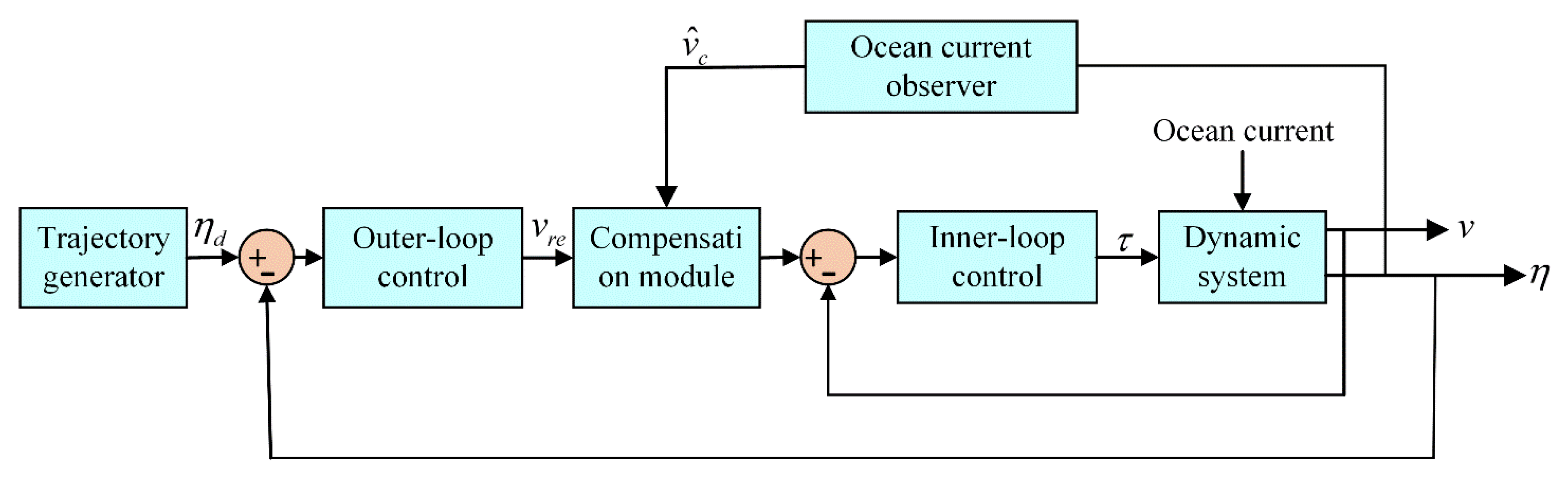
3. Controller Design

3.1. Sliding Mode Control

Conventional SMC is known for its robustness to uncertainty and external disturbances. Let ${\eta }_d$ be the desired position and attitude path of the ROV; the tracking error can be defined as follows:

$${\eta }_e={\eta }_d-\eta$$

(14)

First, the conventional sliding surface is defined by the following equation:

$$S=K{\eta }_e+{\dot{\eta }}_e$$

(15)

where $K\in R^{4\times 4}$ is a constant and positive definite diagonal matrix.

The standard SMC law [44] can be expressed with an equivalent control law and a switching term as

$$\tau ={\tau }_{eq}+{\tau }_{sw}$$

(16)

where τ represents the controllable force acting on the ROVs, and τ_eq and τ_sw symbolize the equivalent control law and the switching term, respectively. The equivalent control law mainly reflects the model information and intuitively represents the dynamics of the controlled object. However, the presence of external disturbances and model uncertainties make the equivalent control law not fully applicable. Hence, the switching term is used to eliminate the difference between the target position and the actual position.

The equivalent control part can be obtained by assuming that the motion is confined to the slipform surface, namely, by deriving Equation (15) and solving for the solution when it is equal to zero, i.e.,

$${\tau }_{eq}=C\left(v\right)v+D\left(v\right)v+g\left(\eta \right)+J\left(\eta \right)M^{-1}\left[c{\dot{\eta }}_e+{\ddot{\eta }}_d-{\dot{J}}_{\psi }\left(\eta \right)v\right]$$

(17)

The switching term of sliding mode control usually uses the switching property of the signum function to eliminate the influence of model uncertainty, but this is also the source of the generation of the chattering phenomenon. To ensure the validity of the subsequent comparison, we choose the hyperbolic tangent function to construct the switching term.

$${\tau }_{sw}=\tanh \left(S/\sigma \right)$$

(18)

The presence of the switching term on the sliding surface causes the chattering problem of the sliding mode control. Therefore, we choose σ to define the thickness of the boundary layer to eliminate the chattering phenomenon. Hence, the construction of the conventional sliding mode control scheme is completed.

$$\tau =C\left(v\right)v+D\left(v\right)v+g\left(\eta \right)+J\left(\eta \right)M^{-1}\left[\rho \arctan \left(S/\sigma \right)+c{\dot{\eta }}_e+{\ddot{\eta }}_d-{\dot{J}}_{\psi }\left(\eta \right)v\right]$$

(19)

Next, a double-loop SMC with an ocean current observer is proposed, and the logic block diagram of the control scheme is shown in Figure 2. The designed control scheme consists of three parts: the reference velocity is generated in the outer-loop controller desired by the error of current position to the target trajectory. Second, the reference velocity is used as the actual control input of the inner-loop controller in order to achieve accurate tracking of the actual position and the reference velocity. Finally, based on the idea of ADRC, we add an ocean current observer between the inner-loop and outer-loop controller to estimate and compensate the disturbance of unknown velocity.

3.2. Outer-Loop (Position Loop) Controller

In the outer loop, the reference velocity is designed to ensure accurate position tracking and is used as a virtual input for velocity tracking in the inner loop. Therefore, the outer-loop sliding surface is defined as

$$S_{\eta }={\eta }_e+K_{\eta }{\displaystyle {\int }_0^t{\eta }_{e}dt}$$

(20)

where $K_{\eta }\in R^{4\times 4}$ is a constant and positive definite diagonal matrix. Choosing the appropriate gain matrix $K_{\eta }$ stabilizes the tracking error on the ideal sliding surface. The derivation of Equation (20) can be obtained as:

$${\dot{S}}_{\eta }={\dot{\eta }}_e+K_{\eta }{\eta }_e$$

(21)

The purpose of designing the outer-loop controller is to generate a virtual control input for the inner-loop controller. The error between the reference velocity $v_{re}$ and true velocity v is $v_e$, as shown in Equation (22).

$$v_e=v_{re}-v$$

(22)

Substituting Equation (22) into Equation (1), we have

$$\dot{\eta }=J\left(\eta \right)v_{re}-J\left(\eta \right)v_e$$

(23)

Combining Equations (21) and (23),

$${\dot{S}}_{\eta }={\dot{\eta }}_d-J\left(\eta \right)v_{re}+J\left(\eta \right)v_e+K_{\eta }{\eta }_e$$

(24)

The virtual control input $v_{re}$, which acts as the reference velocity for the inner loop, is designed as:

$$v_{re}=J^{-1}\left(\eta \right)\left({\dot{\eta }}_d+K_{\eta }{\eta }_e\right)+J^{-1}\left(\eta \right)\rho \tanh \left(S_{\eta }/\sigma \right)$$

(25)

where $\rho \in R^{4\times 4}$ is a definite diagonal matrix that is constant and positive. As with the conventional sliding mode control scheme, σ is defined as the boundary layer thickness of the position loop controller. The stability of the controller is demonstrated in detail in Appendix A.

In the next step, the inner-loop controller is designed such that it will ultimately make the entire system stable.

3.3. Inner-Loop (Velocity Loop) Controller

In the inner loop, the real control input is designed to make the vehicle’s actual velocity precisely track the reference velocity. The inner-loop sliding surface is defined as:

$$s_v=v_e+K_v{\displaystyle {\int }_0^t{v}_{e}dt}$$

(26)

where $K_v\in R^{4\times 4}$ is a constant and positive definite diagonal matrix.

Disregarding the effect of unknown dynamics, deriving Equation (26) and relating it to Equation (5) yields

$$\begin{array}{l}{\dot{s}}_v={\dot{v}}_e+K_v{v}_e\\ ={\dot{v}}_{re}+M^{-1}\left(C_0\left(v\right)v+D_0\left(v\right)v+g_0\left(\eta \right)+\tau \right)+K_v{v}_e\end{array}$$

(27)

Letting ${\dot{s}}_v=0$ and solving the equivalent control law ${\tau }_{eq}$, We can obtain

$${\tau }_{eq}=M_0\left({\dot{v}}_{re}+K_v{v}_e\right)+C_0\left(v\right)v+D_0\left(v\right)v+g_0\left(\eta \right)$$

(28)

Conventional sliding mode control can suffer from chattering problems, which are essentially caused by the discontinuity of the switching term of the controller. Researchers have tried many alternative functions as switching terms and achieved good control results, such as the saturation function, inverse tangent function, and hyperbolic tangent function [36]. In this paper, we apply the hyperbolic tangent function as the switching term:

$${\tau }_{sw}=\Gamma \tanh \left(s_v/\theta \right)$$

(29)

where $\Gamma \in R^{4\times 4}$ is a matrix of diagonal positive definite constants, which are related to the convergence rate of the controller. θ can be regarded as the boundary layer thickness of the inner-loop controller.

If the unknown dynamics and external disturbances are considered, the control equation of ROV is as in Equation (11). However, the effect of unknown dynamics is not considered in the above control process. In order to better achieve precise control effects, we assume that ${\widehat{\tau }}_d$ is an estimate of the unknown dynamics ${\tau }_d$ [45]. Thus, the formula is given as follows:

$${\dot{\widehat{\tau }}}_d=\mathsf{\Psi }{s}_v$$

(30)

where $\mathsf{\Psi }\in R^{4\times 4}$ is a matrix of positive definite diagonal constant. The adaptive term relates the error measure function to the unknown dynamics, and the estimated dynamics will more realistically reflect the actual dynamics than the simple switching term does.

Therefore, the inner-loop controller consists of three components: equivalent control rate (28), unknown kinetic estimation (30), and switching control rate (29). Namely,

$$\tau =M_0\left({\dot{v}}_{re}+K_v{v}_e\right)+C_0\left(v\right)v+D_0\left(v\right)v+g_0\left(\eta \right)+{\displaystyle {\int }_0^t\mathsf{\Psi }{s}_{v}dt}+\Gamma \tanh \left(s_v/\theta \right)$$

(31)

The stability of the inner-loop controller is demonstrated in detail in Appendix B.

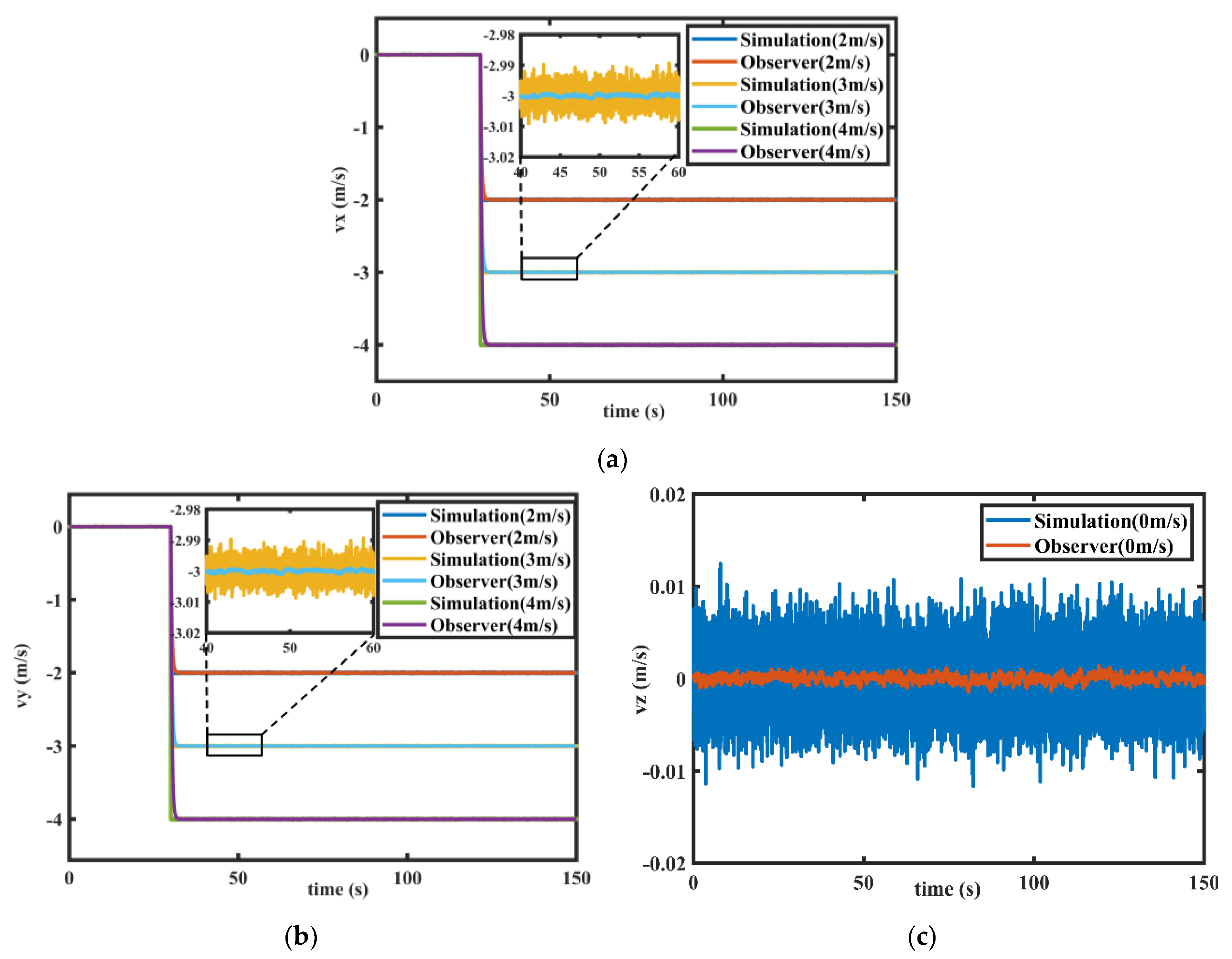
3.4. Ocean Current Observer

From the analysis of the ocean current model, the effect of ocean currents on the ROV body is mainly reflected in the motion of the ROV, which consists of the motion of the body and that of the current. Therefore, the reference velocity $v_{re}$ generated by solving the ROV position of the outer-loop controller also contains two velocity elements. Based on the idea of ADRC, we can design an observer for ocean currents that is unknown and time-varying, so that its estimated ${\widehat{v}}_c$ converge on the unknown current velocity $v_c$. Subsequently, the effect of ocean currents between the inner- and outer-ring controllers is compensated in advance, resulting in highly robust control under large ocean currents.

Adjustment by Equation (12) yields,

$$v_c=\dot{\eta }-J\left(\eta \right)v_r$$

(32)

Therefore, it can be assumed that

$${\dot{\widehat{v}}}_c=\alpha \left[\dot{\eta }-J\left(\eta \right)v_r\right]-\alpha {\widehat{v}}_c$$

(33)

where α is the unknown normal number to be determined, and the slow time-varying current satisfies the assumptions that ${\dot{v}}_c=0m/s^2$, we can derive:

$${\dot{v}}_c^e={\dot{v}}_c-{\dot{\widehat{v}}}_c=0-\left\{\alpha \left[\dot{\eta }-J\left(\eta \right)v_r\right]-\alpha {\widehat{v}}_c\right\}=-\alpha v_c^e$$

(34)

Therefore, the observer designed in this section is exponentially stable. However, it is assumed that the translation velocity of the ROV is only measurable for the surrounding fluid, namely, the inertial system variable $\dot{\eta }$ is not known. Thus, the dummy auxiliary variables are defined here as

$$\omega ={\widehat{v}}_c-\alpha \eta$$

(35)

Similarly, if we define

$$\dot{\omega }=\alpha \left(-\alpha \eta -J\left(\eta \right)v_r\right)-\alpha \omega$$

(36)

eventually, there will be

$$\begin{array}{l}{\dot{v}}_c^e={\dot{v}}_c-{\dot{\widehat{v}}}_c\\ =0-\left(\dot{\omega }+\alpha \dot{\eta }\right)\\ =\left\{\alpha \left(\alpha \eta +J\left(\eta \right)v_r\right)+\alpha \omega \right\}-\alpha \dot{\eta }\\ =\alpha \left(\left(\alpha \eta +\omega \right)-\left(\dot{\eta }-J\left(\eta \right)v_r\right)\right)\\ =\alpha {\widehat{v}}_c-\alpha v_c\\ =-\alpha v_c^e\end{array}$$

(37)

In summary, the designed ocean current observer is

$$\{\begin{array}{l}{\widehat{v}}_c=\omega +\alpha \eta \\ \dot{\omega }=\alpha \left(-\alpha \eta -J\left(\eta \right)v_r\right)-\alpha \omega \end{array}$$

(38)

As the observed value is related to the initial value of the expected position, as shown in Equation (38), the initial value of the expected trajectory can cause excessive initial error of the observer. However, the ROV control position is usually calculated from the origin, so this problem does not affect the control results excessively.

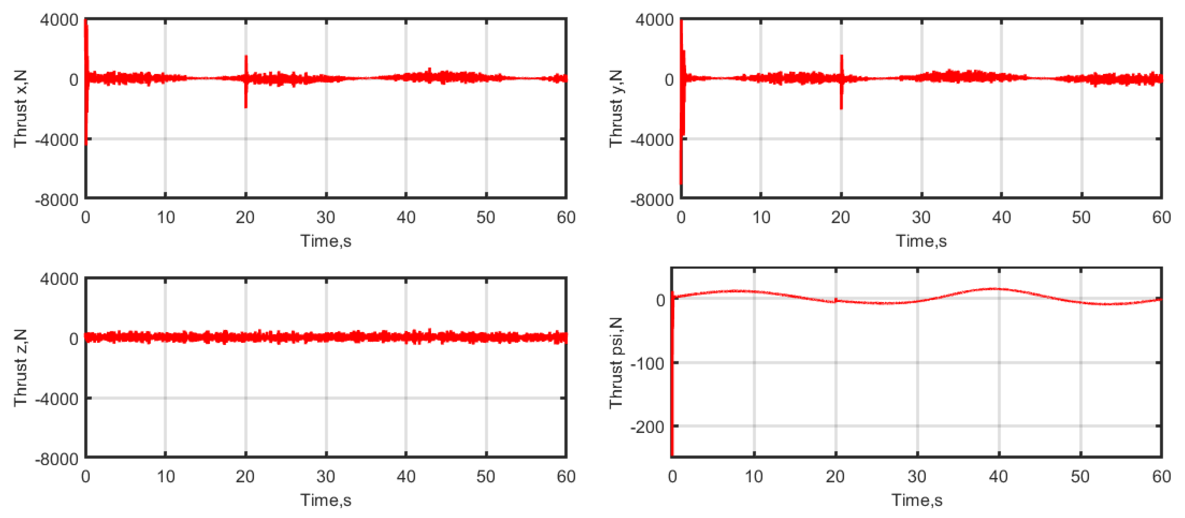
4. Simulation Results and Discussion

The “Lingrui” ROV is an underwater robot independently developed by the research group for underwater cable inspection in the offshore environment. The three-dimensional model and physical prototype of the ROV design are shown in Figure 3, and the actual design parameters are shown in

Table 1. The ROV-designed specifications.

Parameter	Values
dimensions	0.44 m × 0.33 m × 0.30 m
weight	20 kg
volumes	0.0208 m3
operation depth	100 m
communication	power line communication
SoC	raspberry Pi and MK66 microcontroller

. According to the task requirements of submarine cable detection, the ROV is equipped with a GPS positioning module, bathymetry sensor, acceleration sensor, and gyroscope, which can achieve the basic functions of precision navigation, depth perception, attitude perception, automatic control, and video/image acquisition, etc. Hydrodynamic simulation and empirical metric methods were used to obtain the relevant properties of the submarine cable inspection robot, as shown in

Table 2. Nominal parameters of the “Lingrui” ROV.

Parameter	Values	Parameter	Values
$I_z$	4.68 Nms2	$Z_w$	−102.22 N/s
$X_u$	−35.17 N/s	$Z_{\dot{w}}$	−32.73 kg
$X_{\dot{u}}$	−17.25 kg	$Z_{w\left|w\right|}$	−35.62 N2/m2
$X_{u\left|u\right|}$	−9.44 N2/m2	$N_r$	−7.869 N/s
$Y_v$	−42.58 N/s	$N_{\dot{r}}$	−1.538 kg
$Y_{\dot{v}}$	−20.22 kg	$N_{r\left|r\right|}$	−10.65 N2/m2
$Y_{v\left|v\right|}$	−13.53 N2/m2

.

In this section, a simulation was carried out using MATLAB/Simulink^® to demonstrate the effectiveness of the proposed controller. In order to simulate the ROV kinematic process in a real marine environment, the unknown dynamics ${\tau }_d$ in different axes are defined as

$${\tau }_d({\tau }_{dx},{\tau }_{dy},{\tau }_{dz},{\tau }_{dr})=-10\sin \left(0.2t\right)$$

(39)

A slowly variable rheological model is used to approximate the flow field, which can generally be modeled using a first-order Markov process [41]. The velocity of the current in a fixed coordinate system is given by the following equation.

$${\dot{v}}_c\left(t\right)+\mu v_c\left(t\right)=\omega \left(t\right)$$

(40)

where $\mu$ is a positive constant and $\omega \left(t\right)$ is white Gaussian noise. In the simulation, the current velocity is composed of the Gaussian white noise signal and the step signal, and the parameter of the slowly varying current flow field is defined as $\mu =1$. The power spectral density of zero-mean white Gaussian noise is 10⁻⁵.

To illustrate the effectiveness of the proposed control schemes more comprehensively, two trajectory tracking cases were performed: one with a spatial helical desired trajectory and the other with a three-dimensional Dubins desired trajectory, which consists of a vertical straight-line trajectory and a horizontal comb-shaped trajectory. We proceeded as follows.

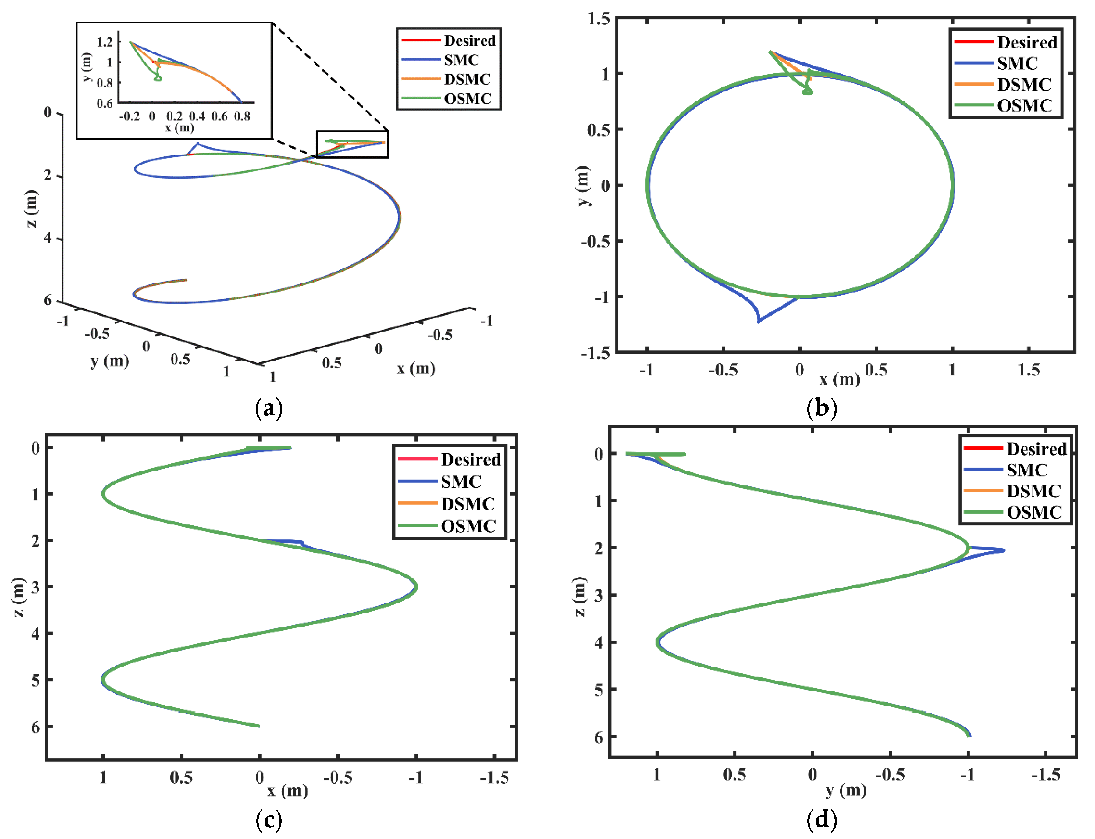
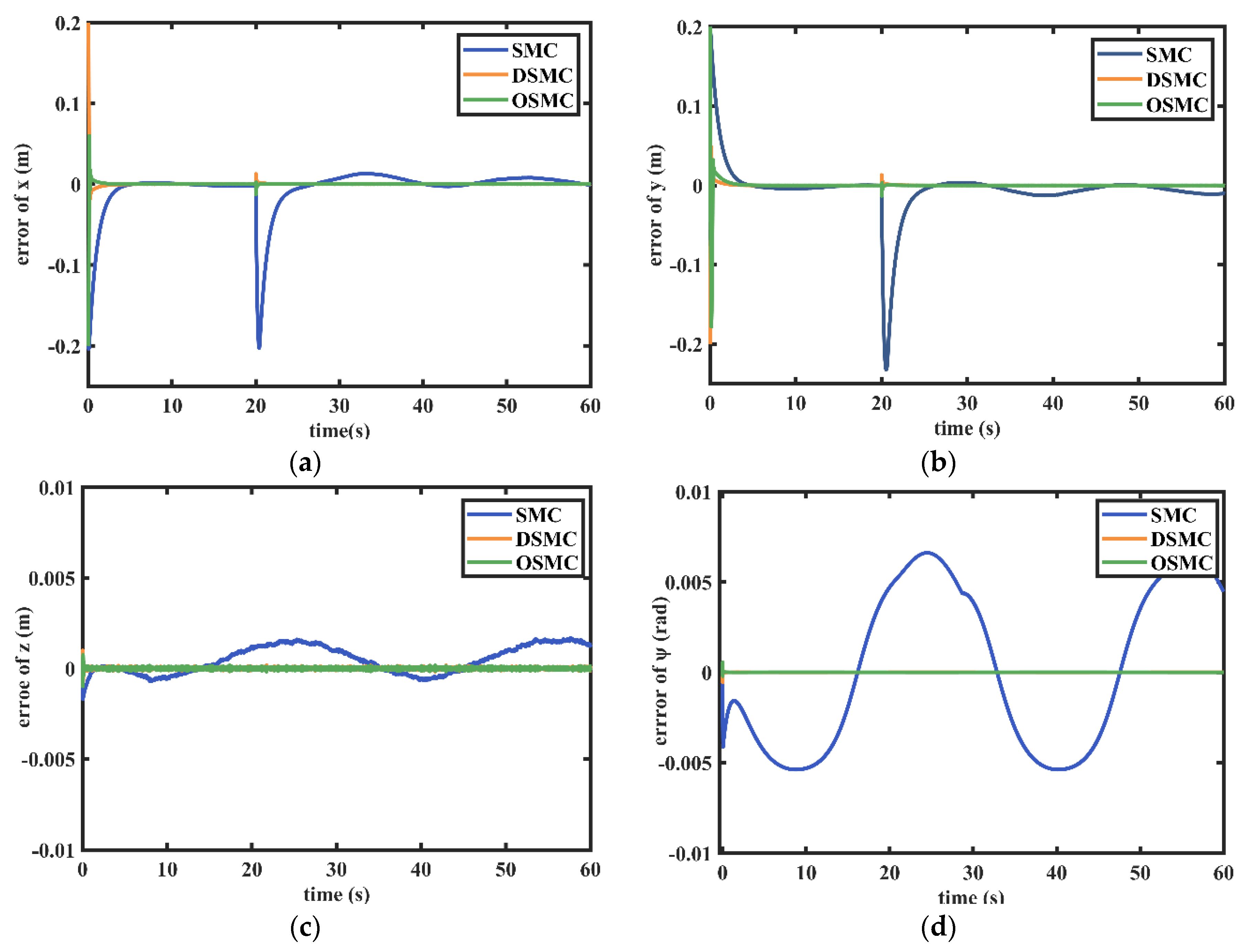
4.1. Controller Performance Comparison

The purpose of this section is to verify that the control method proposed in this paper can effectively control the ROV. The performance of three control schemes were compared under the influence of ocean currents in the marine environment, namely, SMC, double-loop SMC scheme (DSMC), and double-loop SMC scheme with an ocean current observer (OSMC). The desired trajectory in the inertial frame is described as:

$$\{\begin{array}{l}{x}_d\left(t\right)=\sin \left(0.05\pi t\right)m\\ y_d\left(t\right)=\cos \left(0.05\pi t\right)m\\ z_d\left(t\right)=\left(0.1t\right)m\\ {\psi }_d\left(t\right)=\left(0.05\pi t\right)rad\end{array}$$

(41)

The initial position of the ROV is set as $x\left(0\right)=0.2m$, $y\left(0\right)=0.8m$, $z\left(0\right)=0m$, and $\psi \left(0\right)=0rad$, and the other initial conditions are defined as zero at the initial time. In order to ensure the safety of offshore workers, it is generally required that the operation is under sea conditions not exceeding Level 5. Therefore, the ROV simulation is set to run for 60 s, and the simulation step size is 0.001 s. The ocean current velocity is 1.0 m/s, and a slowly variable current disturbance is applied at 30 s. To make the comparison fair and persuasive, corresponding controller parameters for the three control schemes are chosen as the same values: the outer-loop controller parameters are set as $K_p=I_{4\times 4}$ and $\rho =3I_{4\times 4}$; the inner-loop controller parameters are set as $K_v=I_{4\times 4}$, $\mathsf{\Psi }=20I_{4\times 4}$, and $\Gamma =1000I_{4\times 4}$; the ocean current observer parameters are set as $\alpha =3$, and the boundary layer thickness of the sliding mold controller is set as $\theta =0.01$. The conventional SMC parameters are identical to those of the outer-loop controller in the double-loop SMC scheme.

The 3D trajectory of the ROV under the three control schemes and the corresponding position and attitude errors for each degree of freedom are shown in Figure 4 and Figure 5, respectively. It is observed that all three control schemes can achieve accurate trajectory tracking in the presence of a small disturbance of ocean currents. The position and attitude tracking errors are stable in the small boundary region. From the position and attitude tracking errors, it shows that DSMC and OSMC converge to the steady states faster with smaller steady-state errors than the conventional SMC does. In addition, the two schemes have better robustness to the disturbance of ocean currents. Figure 6 shows the thrust output in the four directions controllable by the ROV. It can be seen that the output thrust signal is relatively smooth. After the increase in the ocean current disturbance at 20 s, the output thrust recovers quickly after producing a small fluctuation. This means that the designed controller can effectively eliminate the chattering effect. Due to the shortcomings of the current observer itself, the initial value of the expected trajectory can cause excessive initial error of the observer at the beginning of the simulation. However, the additional error magnitude is small and acceptable.

In order to compare the tracking performance of different control schemes more accurately, this paper defines the following four measurement parameters. The overshoot is defined as the maximum value of the distance between the tracked trajectory and the preset trajectory in 3D space, namely

$$overshoot=\max \left({\eta }_i-{\eta }_{di}\right)$$

(42)

As the goal of trajectory tracking is a time-dependent path, there is no explicit definition of a steady state. We define the boundary layer concept in the process of improving SMC, so we simply assume that the system is in a steady state when the trajectory tracking error is always less than the thickness of the boundary layer. Therefore, the adjustment time is defined as the shortest time from the moment when the current disturbance is applied to the point where the error returns to within 0.01 m. In addition, in order to measure the control performance of the controller during the whole tracking process, the mean absolute error (MAE) and the root-mean-square error (RMSE) are, respectively, defined as,

$$MAE=\frac{1}{n}{\displaystyle \sum _{i=1}^n\left|{\eta }_i-{\eta }_{di}\right|}$$

(43)

$$RMSE=\sqrt{\frac{1}{n}{\displaystyle \sum _{i=1}^n{\left({\eta }_i-{\eta }_{di}\right)}^2}}$$

(44)

The performance parameters of the three control schemes under conventional current disturbance are shown in

Table 3. Comparison of performance of different control schemes under interference.

Performance Comparison	Values	Parameter	Values
Overshoot (m)	0.2038	0.0128	0.0127
Transient Time (s)	16.30	0.007	0.006
MEA (m)	0.0139	0.0005	0.0004
RMSE (m)	0.0315	0.0060	0.0059

. It can be seen that DSMC and OSMC have significant advantages over the common SMC scheme. In terms of response speed, the overshoot of the two double-loop SMC schemes is reduced by more than 93%, and the adjustment time is also reduced from 16.3 s to 0.07 s under conventional ocean current conditions. This effectively ensures fast stability and accurate trajectory tracking of the control schemes. In terms of the trajectory tracking effect, the MAE and RMSE of the two double-loop SMC schemes are reduced by 96% and 80%, respectively. This is crucial for the energy-saving performance of the whole tracking process. The addition of the ocean current observer results in larger tracking errors at the beginning of the simulation. However, with a smaller average tracking error in terms of the overall error, it is possible to achieve stable control and energy saving in the whole process.

4.2. Controller Robustness

In this section, the ROV’s predefined tracking trajectory is a 3-D Dubins desired trajectory. The observation-type ROVs usually operate close to the seafloor, where the geography is mostly complex and uneven terrain. Therefore, the simulated trajectory is chosen for the undulating seabed scenario to illustrate the effectiveness of the scheme. The simulated trajectory contains five parts: the ROV localizes the start position, dives in a straight line, reaches a specified depth, carries out a predefined comb-shaped cruise, and finally returns to the surface. This trajectory contains the common operating conditions for ROV operations, such as depth, fixed altitude, and fixed yaw angle. The desired trajectory in the inertial frame is described as follows:

$$\begin{array}{l}{x}_d\left(t\right)=\{\begin{array}{l}0m,\begin{array}{c}\end{array}0s\le t<30s\\ 0.2\left(t-30\right)m,\begin{array}{c}\end{array}30s\le t<50s\\ 4+\sin \left(0.05\pi \left(t-50\right)\right)m,\begin{array}{c}\end{array}50s\le t<70s\\ 4-0.2\left(t-70\right)m,\begin{array}{c}\end{array}70s\le t<90s\\ -\sin \left(0.05\pi \left(t-90\right)\right)m,\begin{array}{c}\end{array}90s\le t<110s\\ 0.2\left(t-110\right)m,\begin{array}{c}\end{array}110s\le t<130s\\ 4m,\begin{array}{c}\end{array}t\le 130s\end{array}\\ y_d\left(t\right)=\{\begin{array}{l}0.1tm,\begin{array}{c}\end{array}0s\le t<10s\\ 1m,\begin{array}{c}\end{array}10s\le t<50s\\ 2-\cos \left(0.05\pi \left(t-50\right)\right)m,\begin{array}{c}\end{array}50s\le t<70s\\ 3m,\begin{array}{c}\end{array}70s\le t<90s\\ 4-\cos \left(0.05\pi \left(t-90\right)\right)m,\begin{array}{c}\end{array}90s\le t<110s\\ 5m,\begin{array}{c}\end{array}t\le 110s\end{array}\\ z_d\left(t\right)=\{\begin{array}{l}0.2tm,\begin{array}{c}\end{array}0s\le t<30s\\ 6-4\cos \left(0.1\pi \right)+5\sin \left(0.1\pi x\right)+4\cos \left(0.1\pi y\right)m,\begin{array}{c}\end{array}30s\le t<130s\\ 6-4\cos \left(0.1\pi \right)+5\sin \left(0.4\pi \right)+4\cos \left(0.5\pi \right)-0.35\left(t-130\right)m,\begin{array}{c}\end{array}t\le 130s\end{array}\\ {\psi }_d\left(t\right)=\{\begin{array}{l}0rad,\begin{array}{c}\end{array}0s\le t<50s\\ 0.05\pi \left(t-50\right)rad,\begin{array}{c}\end{array}50s\le t<70s\\ \pi rad,\begin{array}{c}\end{array}70s\le t<90s\\ \pi -0.05\pi \left(t-90\right)rad,\begin{array}{c}\end{array}90s\le t<110s\\ 0rad,\begin{array}{c}\end{array}t\le 110s\end{array}\end{array}$$

(45)

The initial conditions of the simulation are set as $x\left(0\right)=0m$, $y\left(0\right)=0m$, $z\left(0\right)=0m$, $\psi \left(0\right)=0rad$, $u\left(0\right)=v\left(0\right)=w\left(0\right)=0m/s$, and $r\left(0\right)=0rad/s$. In order to demonstrate the universality of the control scheme in the marine environment, the simulations are conducted under different ocean currents. The ocean currents are applied when the ROV is moving to the seabed to comb cruise to evaluate the control performance of different controllers under different sizes of ocean currents.

Figure 7 illustrates the trajectories of the three control schemes to make the ROV complete the automatic navigation of a given path under different ocean current conditions. It can be observed that as the current disturbance increases, the conventional SMC scheme fails first, followed by the double-loop SMC scheme, and the double-loop SMC scheme with an ocean current observer remains effective all the time. It can also be noticed that the conventional SMC scheme fails completely in large currents with track tracking. The failure of the double-loop SMC scheme is mainly due to the presence of steady-state errors that cannot be eliminated. Figure 8 shows the comparison between the simulated imposed current disturbances and the estimated results of the current observer. The ocean current observer can achieve an accurate estimation of the ambient current based on the position of the ROV and accelerometer data. After that, velocity compensation is applied between the inner loop and outer loop of the double-loop SMC to achieve stable control of the ROV under uncertain large current disturbances.

Figure 9 summarizes the root-mean-square error (RMSE) of the trajectory tracking for different control schemes under the condition that the current disturbance is within 5 m/s. Compared with the completely failed sliding mode control and the double-loop sliding mode control scheme with large tracking errors, the overall tracking error increases with the ocean currents. However, by adding the current observer link, the overall tracking error is always kept within a small error range. The results show that the presence of disturbance force reduces the performance of the observer, and although the disturbance force modeling cannot fully characterize the control, due to the current disturbance, modeling the disturbance force and compensating the observer is an effective method to improve the observer accuracy without modifying the observer parameters. The sliding mode control scheme combining the idea of ADRC and the double-loop structure has better control accuracy and stability, and it effectively improves the robustness to ocean current disturbances without increasing the computational effort excessively. Huang and Yang’s study [36] shows that the complicated calculation process of the fuzzy sliding mode method causes an increase in computation time. Compared with the high-complexity control schemes such as neural network-based PID control or fuzzy sliding mode control with large computational effort, it is more practical in ROV systems with limited computational power at the present stage.

5. Conclusions

Achieving ROV trajectory tracking under large ocean current disturbances is challenging work. For this reason, a double-loop sliding mode control scheme with an ocean current observer was proposed in this paper. The main reason for the chattering phenomenon in the conventional SMC is that the position error and velocity error change at different rates. Unlike the conventional SMC that only considers velocity matching, the double-loop control structure could realize the simultaneous control effect of position and velocity. The dual-loop SMC scheme could reduce the overshoot error by 93% compared with the conventional SMC under conventional ocean current conditions. The adjustment time was also reduced from 16.3 s to 0.07 s, which effectively ensured that the ROV achieved accurate trajectory tracking performance and greatly improved the response time of the controller. Therefore, the combination of the double-loop structure and SMC has good adaptability and application prospects for the ROVs’ system.

In addition, the role of ocean currents with ROV systems is often complex and difficult to define clearly, so we defined ocean currents as the ambient velocity. This also made us pay extra attention to the velocity error problem in the control scheme. Based on this consideration, an ocean current observer designed according to the idea of ADRC was introduced to estimate and compensate for the unknown current disturbances. Simulation results showed that the current observer could effectively predict the magnitude of the currents and achieve the purpose of pre-compensation. It showed an excellent trajectory tracking effect under different sizes of current disturbances.

Regarding the future research work, the pool experiment and engineering practice of the control methods mentioned in this paper are certainly the most important elements. The experimental results will be a valid example for this paper and a basis for future research. In addition, the latest research related to ROVs and SMC, such as dynamic sliding mode control, multiple sliding modes, and other methods are also our future research interests.

References

1. Yuh, J. Design and Control of Autonomous Underwater Robots: A Survey. Auton. Robot. 2000, 8, 7–24. [Google Scholar] [CrossRef]
2. Sahoo, A.; Dwivedy, S.K.; Robi, P.S. Advancements in the field of autonomous underwater vehicle. Ocean Eng. 2019, 181, 145–160. [Google Scholar] [CrossRef]
3. Zhang, J.Z.; Wei, Y.J.; Bi, F.Y.; Cao, W. Position-tracking control of underactuated autonomous underwater vehicles in the presence of unknown ocean currents. IET Control Theory Appl. 2010, 4, 2369–2380. [Google Scholar] [CrossRef]
4. Alonge, F.; D’Ippolito, F.; Raimondi, F.M. Trajectory tracking of underactuated underwater vehicles. In Proceedings of the 40th IEEE Conference on Decision and Control, Orlando, FL, USA, 4–7 December 2001; pp. 4421–4426. [Google Scholar] [CrossRef]
5. Beccario, C. Ocean Currents Data in the OSCAR Archive. Available online: https://earth.nullschool.net/ (accessed on 28 November 2020).
6. Shome, S.N.; Nandy, S.; Pal, D.; Das, S.K.; Vadali, S.R.K.; Basu, J.; Ghosh, S. Development of Modular Shallow Water AUV: Issues & Trial Results. J. Inst. Eng. India Ser. C 2012, 93, 217–228. [Google Scholar] [CrossRef]
7. Hernández-Alvarado, R.; García-Valdovinos, L.; Salgado-Jiménez, T.; Gómez-Espinosa, A.; Fonseca-Navarro, F. Neural Network-Based Self-Tuning PID Control for Underwater Vehicles. Sensors 2016, 16, 1429. [Google Scholar] [CrossRef] [Green Version]
8. Chu, Z.; Xiang, X.; Zhu, D.; Luo, C.; Xie, D. Adaptive trajectory tracking control for remotely operated vehicles considering thruster dynamics and saturation constraints. Isa Trans. 2020, 100, 28–37. [Google Scholar] [CrossRef] [PubMed]
9. Maalouf, D.; Chemori, A.; Creuze, V. L1 Adaptive depth and pitch control of an underwater vehicle with real-time experiments. Ocean Eng. 2015, 98, 66–77. [Google Scholar] [CrossRef] [Green Version]
10. Do, K.D. Robust adaptive tracking control of underactuated ODINs under stochastic sea loads. Robot. Auton. Syst. 2015, 72, 152–163. [Google Scholar] [CrossRef]
11. Wang, Y.; Zhang, M.; Wilson, P.A.; Liu, X. Adaptive neural network-based backstepping fault tolerant control for underwater vehicles with thruster fault. Ocean Eng. 2015, 110, 15–24. [Google Scholar] [CrossRef]
12. Repoulias, F.; Papadopoulos, E. Planar trajectory planning and tracking control design for underactuated AUVs. Ocean Eng. 2007, 34, 1650–1667. [Google Scholar] [CrossRef]
13. Londhe, P.S.; Patre, B.M. Adaptive fuzzy sliding mode control for robust trajectory tracking control of an autonomous underwater vehicle. Intell. Serv. Robot. 2019, 12, 87–102. [Google Scholar] [CrossRef]
14. García-Valdovinos, L.G.; Fonseca-Navarro, F.; Aizpuru-Zinkunegi, J.; Salgado-Jiménez, T.; Gómez-Espinosa, A.; Cruz-Ledesma, J.A. Neuro-Sliding Control for Underwater ROV’s Subject to Unknown Disturbances. Sensors 2019, 19, 2943. [Google Scholar] [CrossRef] [PubMed] [Green Version]
15. Yan, Y.; Yu, S. Sliding mode tracking control of autonomous underwater vehicles with the effect of quantization. Ocean Eng. 2018, 151, 322–328. [Google Scholar] [CrossRef]
16. Xu, J.; Wang, M.; Qiao, L. Dynamical sliding mode control for the trajectory tracking of underactuated unmanned underwater vehicles. Ocean Eng. 2015, 105, 54–63. [Google Scholar] [CrossRef]
17. Yang, Y.; Yang, Y.; Mu, W.; Xing, S. Control strategy of low energy consumption rising and diving motion based on buoyancy actuation system. J. Huazhong Univ. Sci. Tech. Nat. Sci. Ed. 2019, 47, 57–62. [Google Scholar] [CrossRef]
18. Yu, C.; Xiang, X.; Lapierre, L.; Zhang, Q. Nonlinear guidance and fuzzy control for three-dimensional path following of an underactuated autonomous underwater vehicle. Ocean Eng. 2017, 146, 457–467. [Google Scholar] [CrossRef] [Green Version]
19. Shojaei, K. Three-dimensional neural network tracking control of a moving target by underactuated autonomous underwater vehicles. Neural Comput. Appl. 2019, 31, 509–521. [Google Scholar] [CrossRef]
20. Wang, Z.; Guo, S.; Shi, L.; Pan, S.; He, Y. The application of PID control in motion control of the spherical amphibious robot. In Proceedings of the 2014 IEEE International Conference on Mechatronics and Automation, Tianjin, China, 3–6 August 2014; pp. 1901–1906. [Google Scholar] [CrossRef]
21. Vu, M.T.; Le Thanh, H.N.N.; Huynh, T.; Thang, Q.; Duc, T.; Hoang, Q.; Le, T. Station-Keeping Control of a Hovering Over-Actuated Autonomous Underwater Vehicle Under Ocean Current Effects and Model Uncertainties in Horizontal Plane. IEEE Access 2021, 9, 6855–6867. [Google Scholar] [CrossRef]
22. Nhu Ngoc Thanh, H.L.; Vu, M.T.; Nguyen, N.P.; Mung, N.X.; Hong, S.K. Finite-Time Stability of MIMO Nonlinear Systems Based on Robust Adaptive Sliding Control: Methodology and Application to Stabilize Chaotic Motions. IEEE Access 2021, 9, 21759–21768. [Google Scholar] [CrossRef]
23. Alattas, K.A.; Mobayen, S.; Din, S.U.; Asad, J.H.; Fekih, A.; Assawinchaichote, W.; Vu, M.T. Design of a Non-Singular Adaptive Integral-Type Finite Time Tracking Control for Nonlinear Systems with External Disturbances. IEEE Access 2021, 9, 102091–102103. [Google Scholar] [CrossRef]
24. Fossen, T.I. Guidance and Control of Ocean Vehicles; John Wiley & Sons: New York, NY, USA, 1994. [Google Scholar]
25. Refsnes, J.E.; Sorensen, A.J.; Pettersen, K.Y. Model-Based Output Feedback Control of Slender-Body Underactuated AUVs: Theory and Experiments. IEEE T. Contr. Syst. T. 2008, 16, 930–946. [Google Scholar] [CrossRef]
26. Haghi, P.; Naraghi, M.; Vanini, S.A.S. Adaptive Position and Attitude Tracking of an AUV in the Presence of Ocean Current Disturbances. In Proceedings of the 16th IEEE International Conference on Control Applications, Singapore, 1–3 October 2007; pp. 741–746. [Google Scholar] [CrossRef]
27. Han, J. From PID to Active Disturbance Rejection Control. IEEE T. Ind. Electron. 2009, 56, 900–906. [Google Scholar] [CrossRef]
28. Lamraoui, H.C.; Qidan, Z. Path following control of fully-actuated autonomous underwater vehicle in presence of fast-varying disturbances. Appl. Ocean Res. 2019, 86, 40–46. [Google Scholar] [CrossRef]
29. Thanh, H.L.N.N.; Vu, M.T.; Mung, N.X.; Nguyen, N.P.; Phuong, N.T. Perturbation Observer-Based Robust Control Using a Multiple Sliding Surfaces for Nonlinear Systems with Influences of Matched and Unmatched Uncertainties. Mathematics 2020, 8, 1371. [Google Scholar] [CrossRef]
30. Jakovljević, B.; Lino, P.; Maione, G. Control of double-loop permanent magnet synchronous motor drives by optimized fractional and distributed-order PID controllers. Eur. J. Control 2021, 58, 232–244. [Google Scholar] [CrossRef]
31. Zhong, B.; Jin, Z.; Zhu, J.; Wang, Z.; Sun, L. Double closed-loop control of a trans-scale precision positioning stage based on the inertial stick-slip driving. Sens. Actuators A Phys. 2019, 297, 111547. [Google Scholar] [CrossRef]
32. Xue, J.; Jiao, X.; Sun, Z. ESO-Based Double Closed-loop Servo Control for Automobile Electronic Throttle. IFAC-Pap. 2018, 51, 979–983. [Google Scholar] [CrossRef]
33. Mu, W.; Zou, Z.; Liu, G.; Yang, Y.; Shi, L. Depth Control Method of Profiling Float Based on an Improved Double PD Controller. IEEE Access 2019, 7, 43258–43268. [Google Scholar] [CrossRef]
34. Mu, W.; Zou, Z.; Sun, H.; Yang, Y. A Control Strategy with Low Power Consumption for Buoyancy Regulation System of Submersibles. J. Xian Jiaotong Univ. 2018, 52, 44–49. [Google Scholar] [CrossRef]
35. Qiao, L.; Zhang, W. Double-Loop Integral Terminal Sliding Mode Tracking Control for UUVs With Adaptive Dynamic Compensation of Uncertainties and Disturbances. IEEE J. Ocean. Eng. 2019, 44, 29–53. [Google Scholar] [CrossRef]
36. Huang, B.; Yang, Q. Double-loop sliding mode controller with a novel switching term for the trajectory tracking of work-class ROVs. Ocean Eng. 2019, 178, 80–94. [Google Scholar] [CrossRef]
37. Yan, Z.; Wang, M.; Xu, J. Robust adaptive sliding mode control of underactuated autonomous underwater vehicles with uncertain dynamics. Ocean Eng. 2019, 173, 802–809. [Google Scholar] [CrossRef]
38. Rojsiraphisal, T.; Mobayen, S.; Asad, J.H.; Vu, M.T.; Chang, A.; Puangmalai, J. Fast Terminal Sliding Control of Underactuated Robotic Systems Based on Disturbance Observer with Experimental Validation. Mathematics 2021, 9, 1935. [Google Scholar] [CrossRef]
39. Vu, M.T.; Van, M.; Bui, D.H.P.; Do, Q.T.; Huynh, T.; Lee, S.; Choi, H. Study on Dynamic Behavior of Unmanned Surface Vehicle-Linked Unmanned Underwater Vehicle System for Underwater Exploration. Sensors 2020, 20, 1329. [Google Scholar] [CrossRef] [PubMed] [Green Version]
40. Vu, M.T.; Choi, H.S.; Kang, J.; Ji, D.H.; Jeong, S.K. A study on hovering motion of the underwater vehicle with umbilical cable. Ocean Eng. 2017, 135, 137–157. [Google Scholar] [CrossRef]
41. Li, X.; Zhao, M.; Ge, T. A Nonlinear Observer for Remotely Operated Vehicles with Cable Effect in Ocean Currents. Appl. Sci. 2018, 8, 867. [Google Scholar] [CrossRef] [Green Version]
42. Vu, M.T.; Le, T.; Thanh, H.L.N.N.; Huynh, T.; Van, M.; Hoang, Q.; Do, T.D. Robust Position Control of an Over-actuated Underwater Vehicle under Model Uncertainties and Ocean Current Effects Using Dynamic Sliding Mode Surface and Optimal Allocation Control. Sensors 2021, 21, 747. [Google Scholar] [CrossRef]
43. García-Valdovinos, L.G.; Salgado-Jiménez, T.; Bandala-Sánchez, M.; Nava-Balanzar, L.; Hernández-Alvarado, R.; Cruz-Ledesma, J.A. Modelling, Design and Robust Control of a Remotely Operated Underwater Vehicle. Int. J. Adv. Robot. Syst. 2014, 11, 1. [Google Scholar] [CrossRef] [Green Version]
44. Soylu, S.; Buckham, B.J.; Podhorodeski, R.P. A chattering-free sliding-mode controller for underwater vehicles with fault-tolerant infinity-norm thrust allocation. Ocean Eng. 2008, 35, 1647–1659. [Google Scholar] [CrossRef]
45. Qiao, L.; Zhang, W. Double-loop chattering-free adaptive integral sliding mode control for underwater vehicles. In Proceedings of the OCEANS 2016—Shanghai, Shanghai, China, 10–13 April 2016; pp. 1–6. [Google Scholar] [CrossRef]
Figure 1. Two coordinated frames used in the modeling and analysis of ROVs.
Jmse 09 01000 g001
Figure 2. The logic block diagram for the double-loop SMC with an ocean current observer.
Jmse 09 01000 g002
Figure 3. Model of “Lingrui” ROV: (a) 3D model with thruster arrangement; (b) physical model.
Jmse 09 01000 g003
Figure 4. The 3D trajectory tracking results of the ROV under the three control schemes: (a) XYZ 3D trajectory; (b) XY plane trajectory; (c) XZ plane trajectory; (d) YZ plane trajectory.
Jmse 09 01000 g004
Figure 5. Tracking errors for the position and attitude of the ROV associated with the three control schemes: (a) tracking error of position x; (b) tracking error of position y; (c) tracking error of position z; and (d) tracking error of attitude Ψ.
Jmse 09 01000 g005
Figure 6. Output thrust on four controllable degrees of freedom.
Jmse 09 01000 g006
Figure 7. The 3D trajectory tracking results of the ROV under different ocean current conditions: (a) trajectory tracking results under the condition of ocean current velocity of 2 m/s; (b) trajectory tracking results under the condition of ocean current velocity of 3 m/s; (c) trajectory tracking results under the condition of ocean current velocity of 4 m/s.
Jmse 09 01000 g007
Figure 8. The comparison of ocean current observer estimates with actual currents: (a) comparison of real and observed values of ocean currents of different sizes in the X-direction; (b) comparison of real and observed values of ocean currents of different sizes in the Y-direction; (c) comparison of real and observed values of ocean currents in the Z-direction.
Jmse 09 01000 g008
Figure 9. The variation in RMSE of the tracking trajectory for three control schemes, when ocean current velocities vary between 0 m/s and 5 m/s.
Jmse 09 01000 g009