
What Speleothems Tell Us about Long-Term Rainfall Oscillation throughout the Holocene on a Planetary Scale


Abstract
:1. Introduction
1.1. State of the Art
1.2. Rainfall Oscillation
1.3. Subtropical Gyres
1.4. The Speleothems, Witnesses of the Evolution of Precipitation
2. Materials and Methods
2.1. Methodological Approach
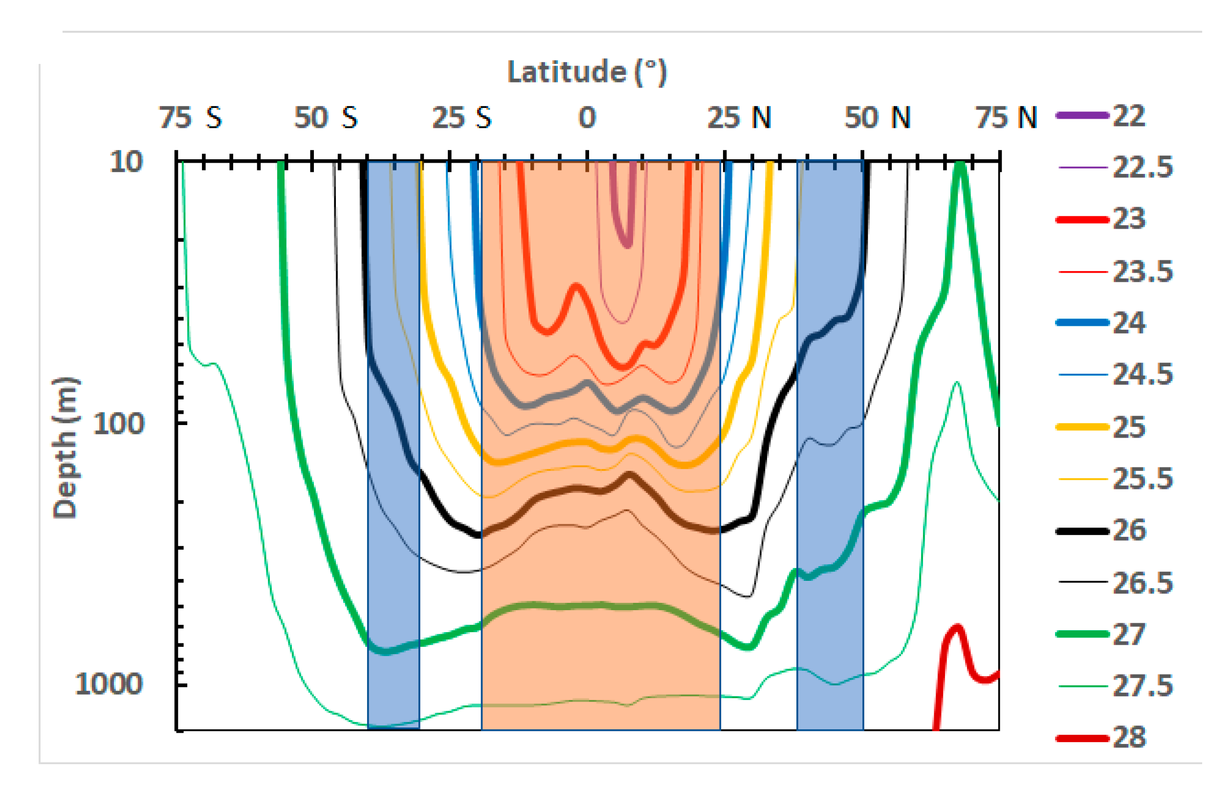
2.2. Ocean Stratification
2.3. Data
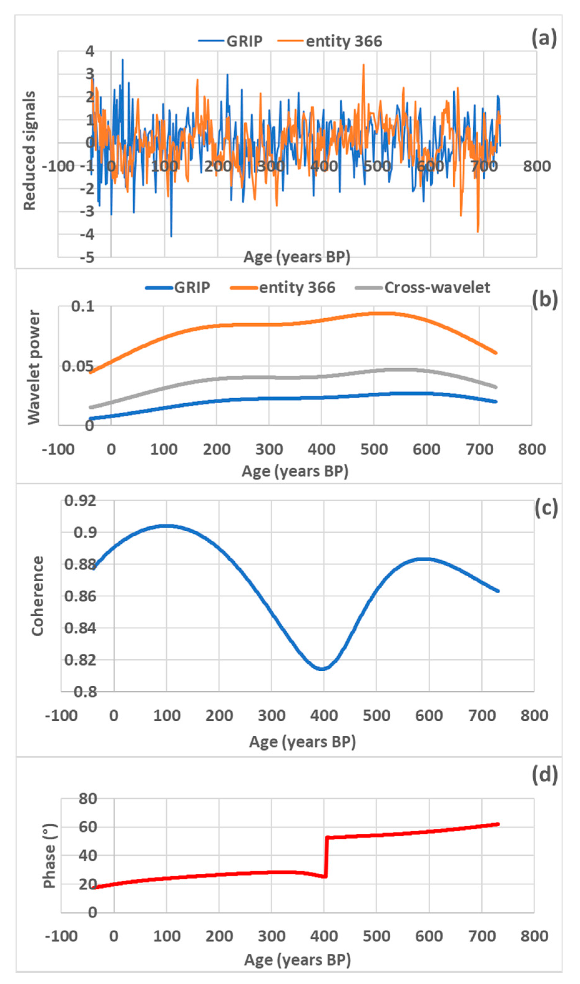
2.4. Wavelet Power, Coherence, and Phase Difference
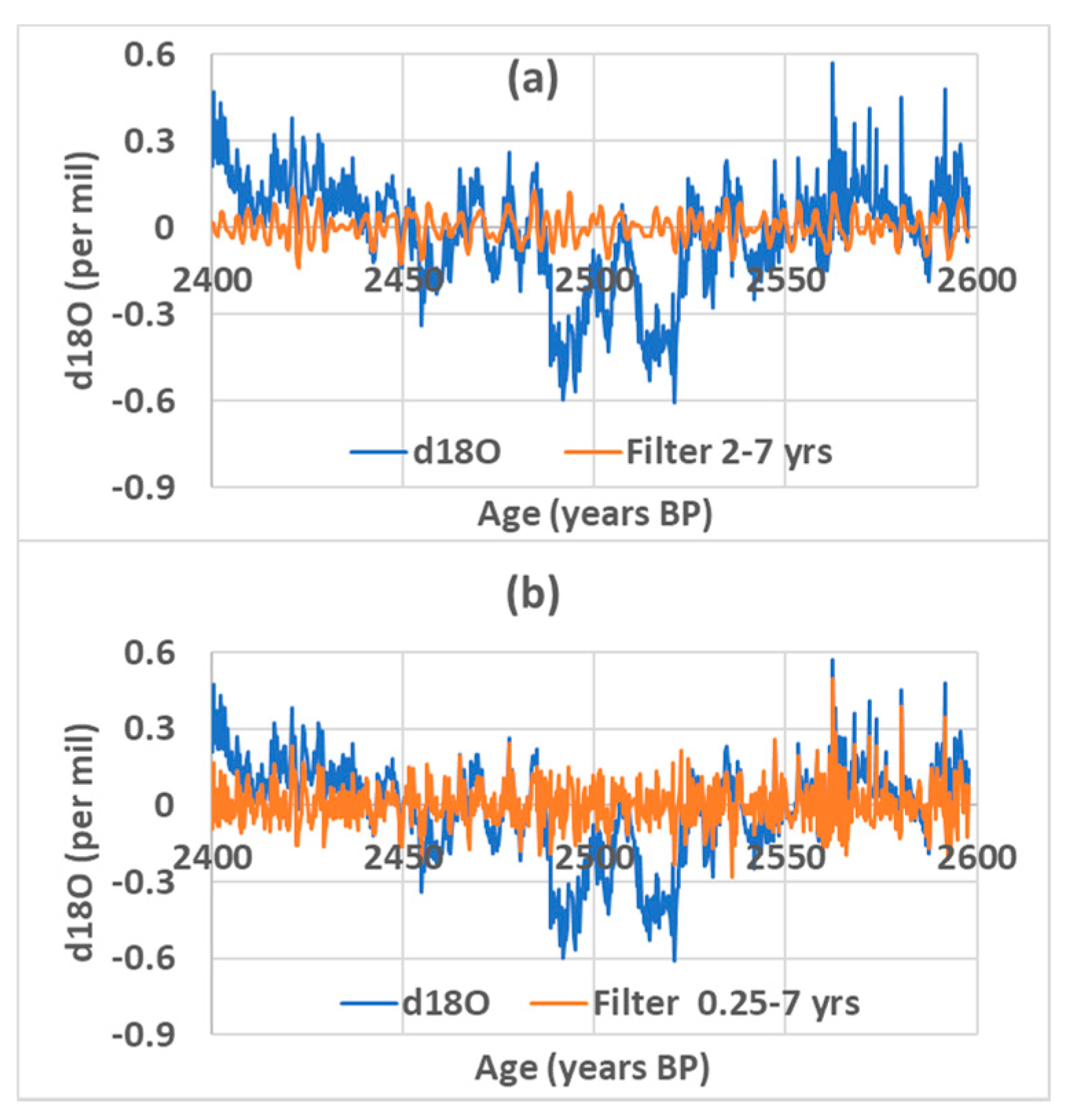
2.5. Filtering
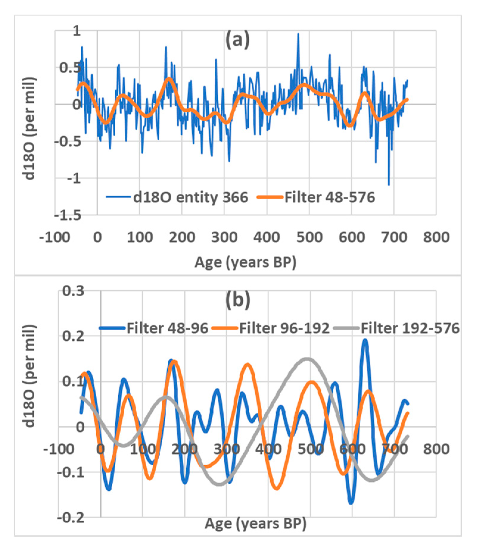
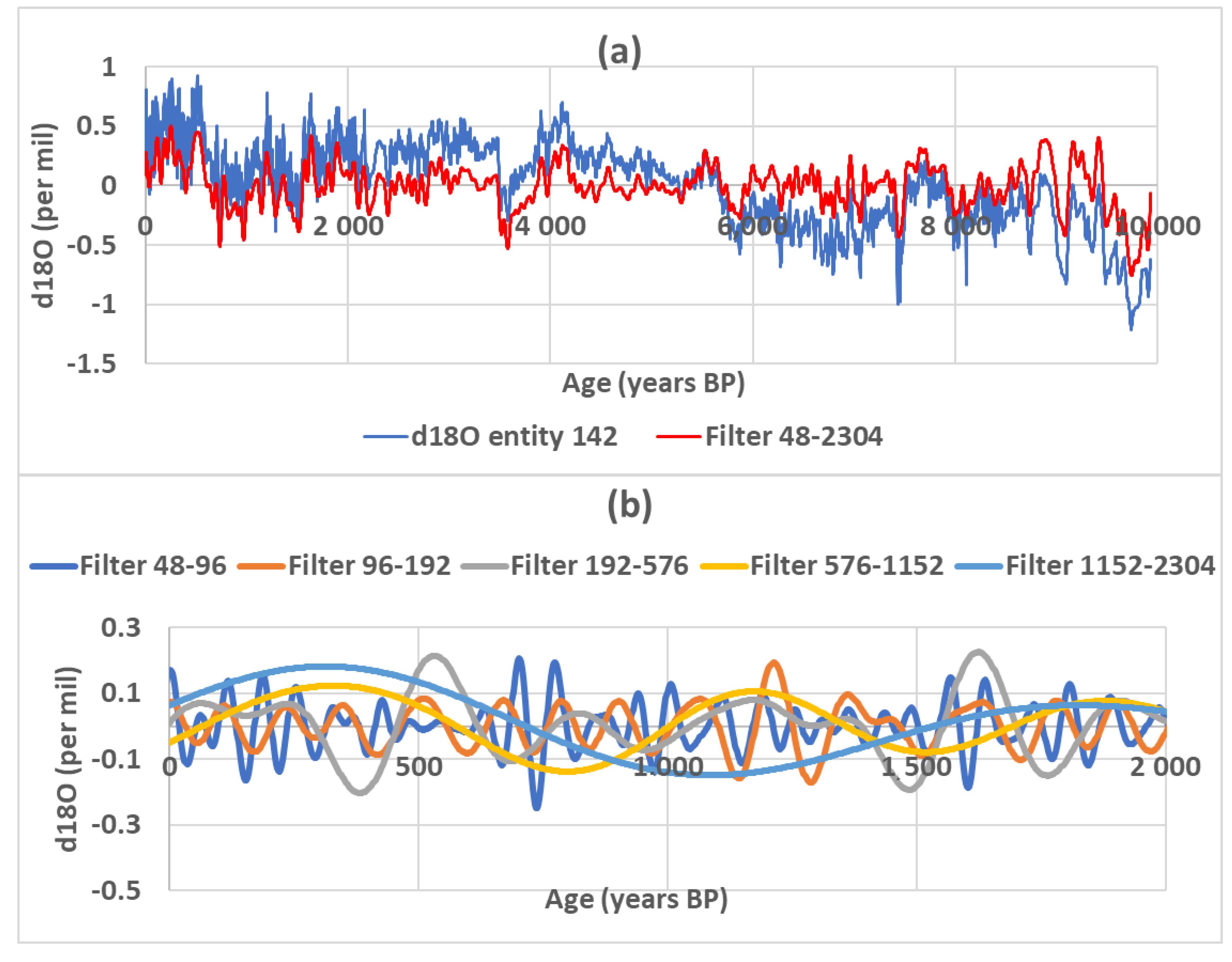
2.6. Examples
- entity 142 (COMNISPA II), site 58 (Spannagel cave), latitude 47.08° N, longitude 11.67° E, elevation 2310 m, geology marble, rock age Jurassic, Jens Fohlmeister [26];
- entity 366 (S3), site 170 (Defore cave), latitude 17.1667° N, longitude 54.0833° E, elevation 150 m, geology limestone, rock age unknown, Drew Lorrey [27];
- entity 285 (BA03_highres), site 116 (Bukit Assam cave), latitude 4.03° N, longitude 114.8° E, elevation 150 m, geology unknown, rock age unknown, Jun Hu [28].
2.6.1. Speleothems Reflecting Long-Period Rainfall Oscillation
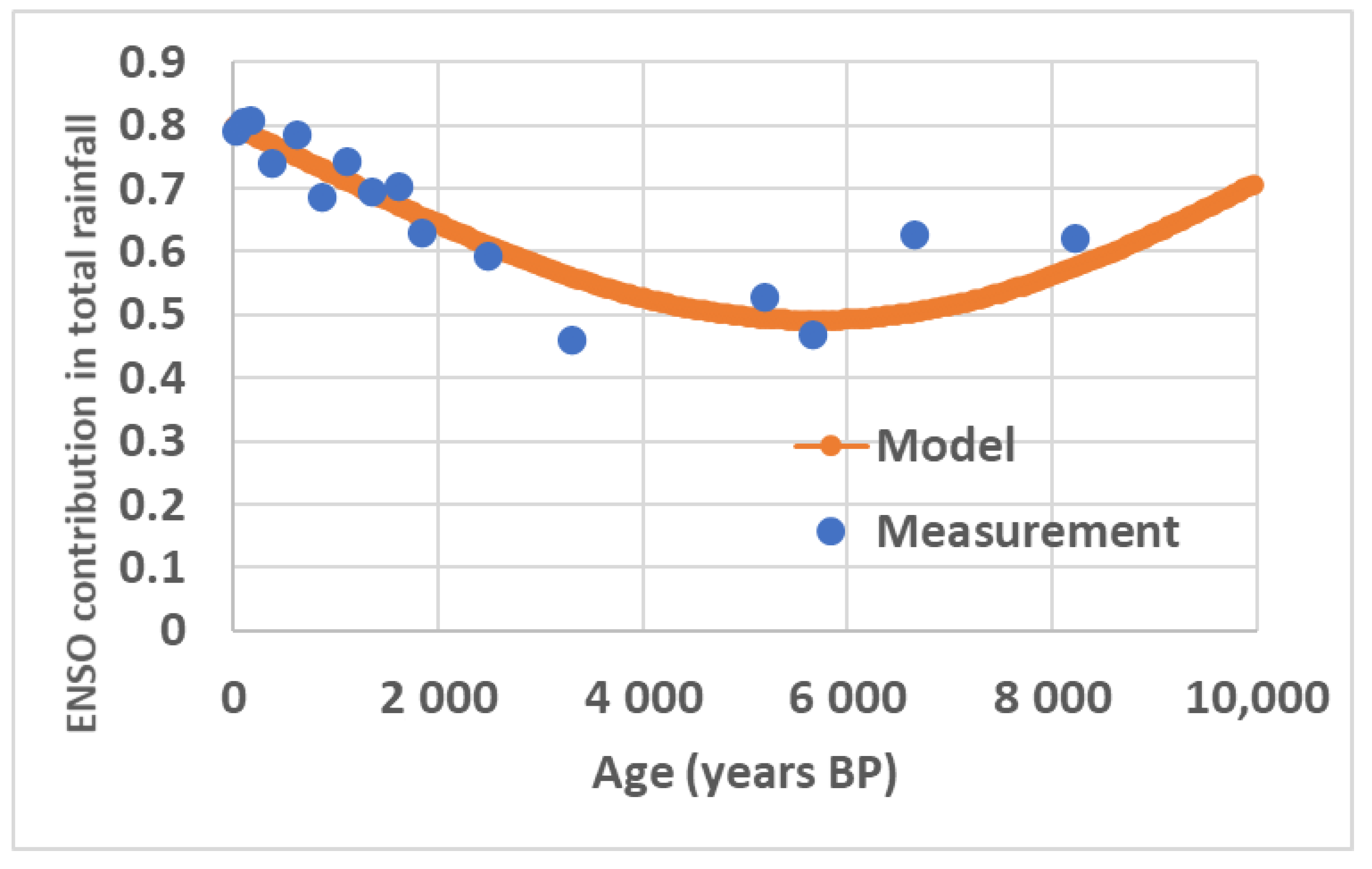
2.6.2. Speleothems Reflecting the Contribution of ENSO to Total Precipitation
2.7. The Scope of the Study
3. Results
3.1. Seven Regions to Result in the Climatic Response of Speleothems
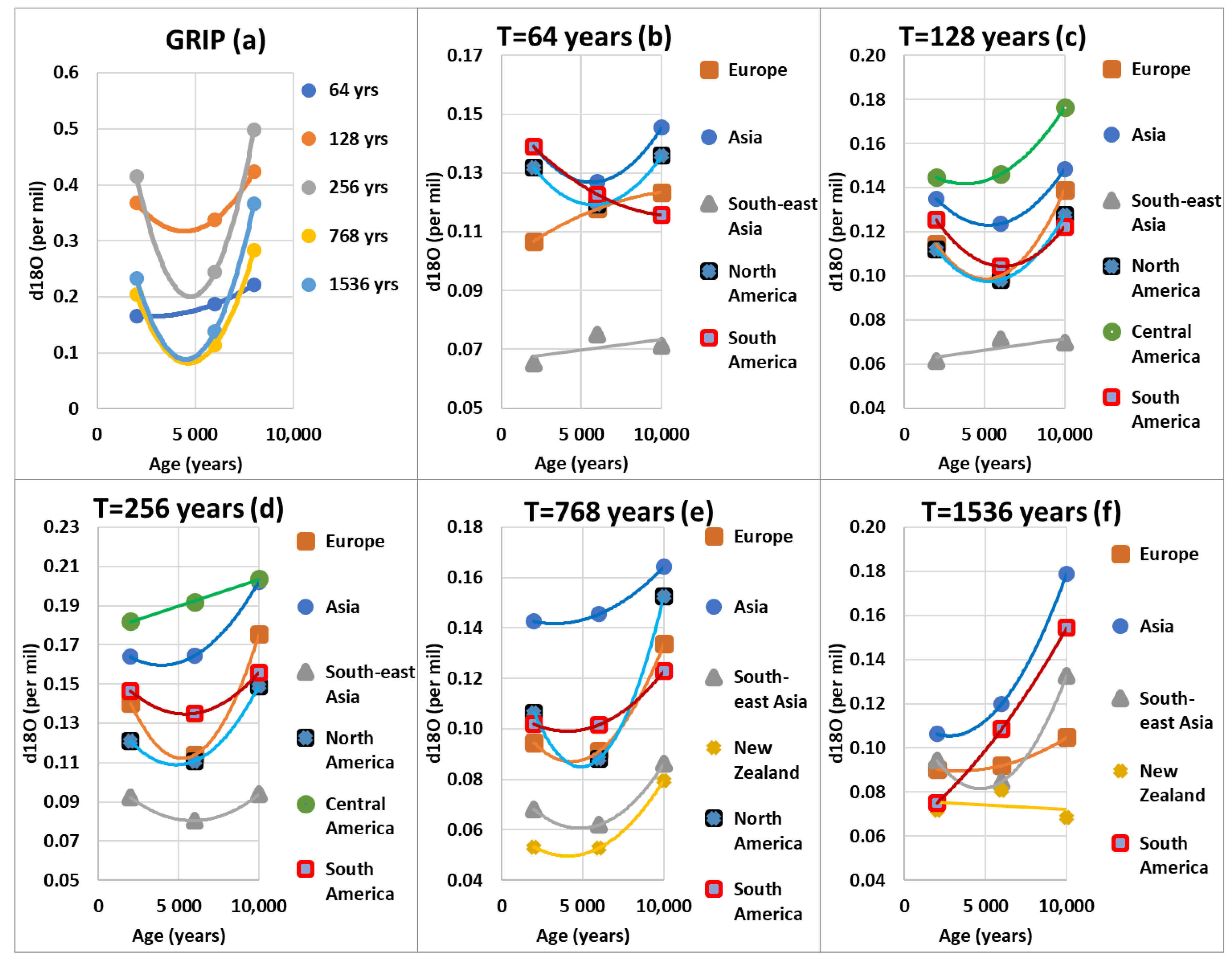
3.2. Variations in the δ18O Composition of Speleothems from the Seven Regions for the First Five Subharmonic Modes
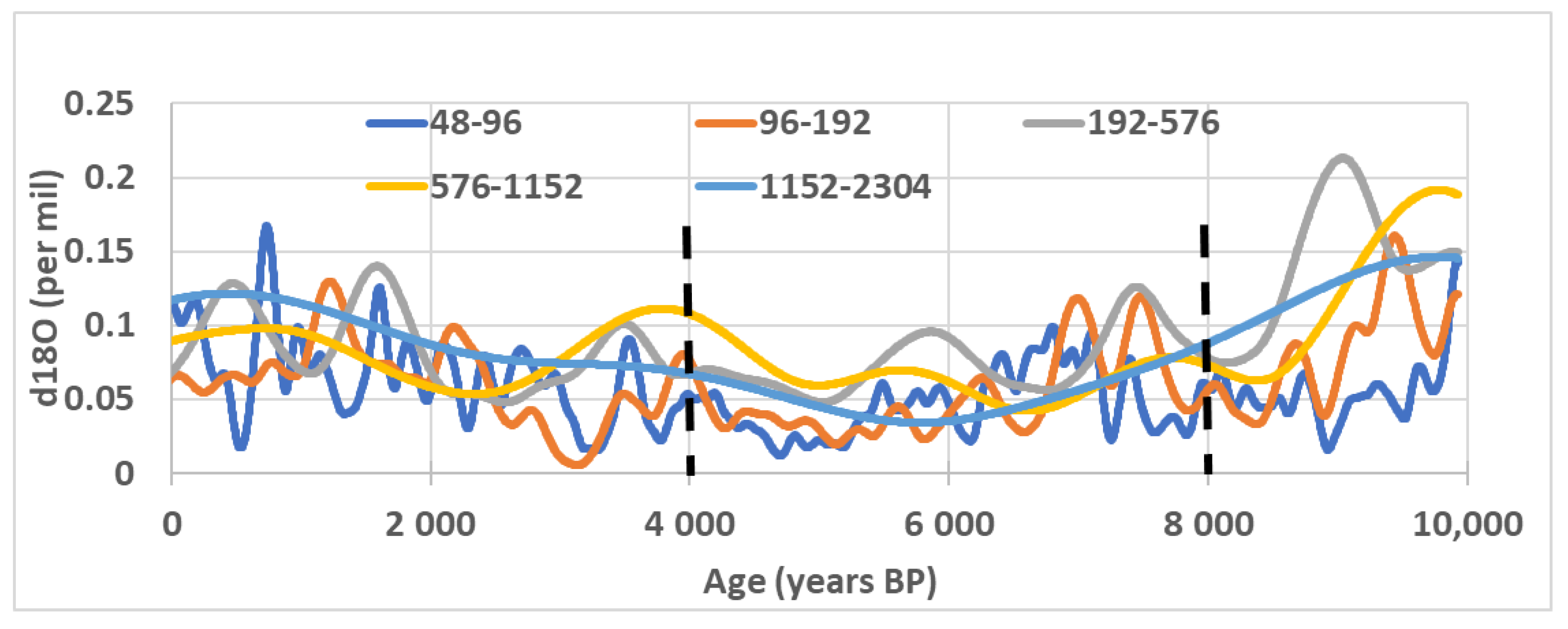
3.2.1. Subharmonic Mode (Band 48–96 Years, = 64 Years)
3.2.2. Subharmonic Mode (Band 96–192 Years, = 128 Years)
3.2.3. Subharmonic Mode (Band 192–576 Years, = 256 Years)
3.2.4. Subharmonic Mode (Band 576–1152 Years, = 768 Years)
3.2.5. Subharmonic Mode (Band 1152–2304 Years, = 1536 Years)
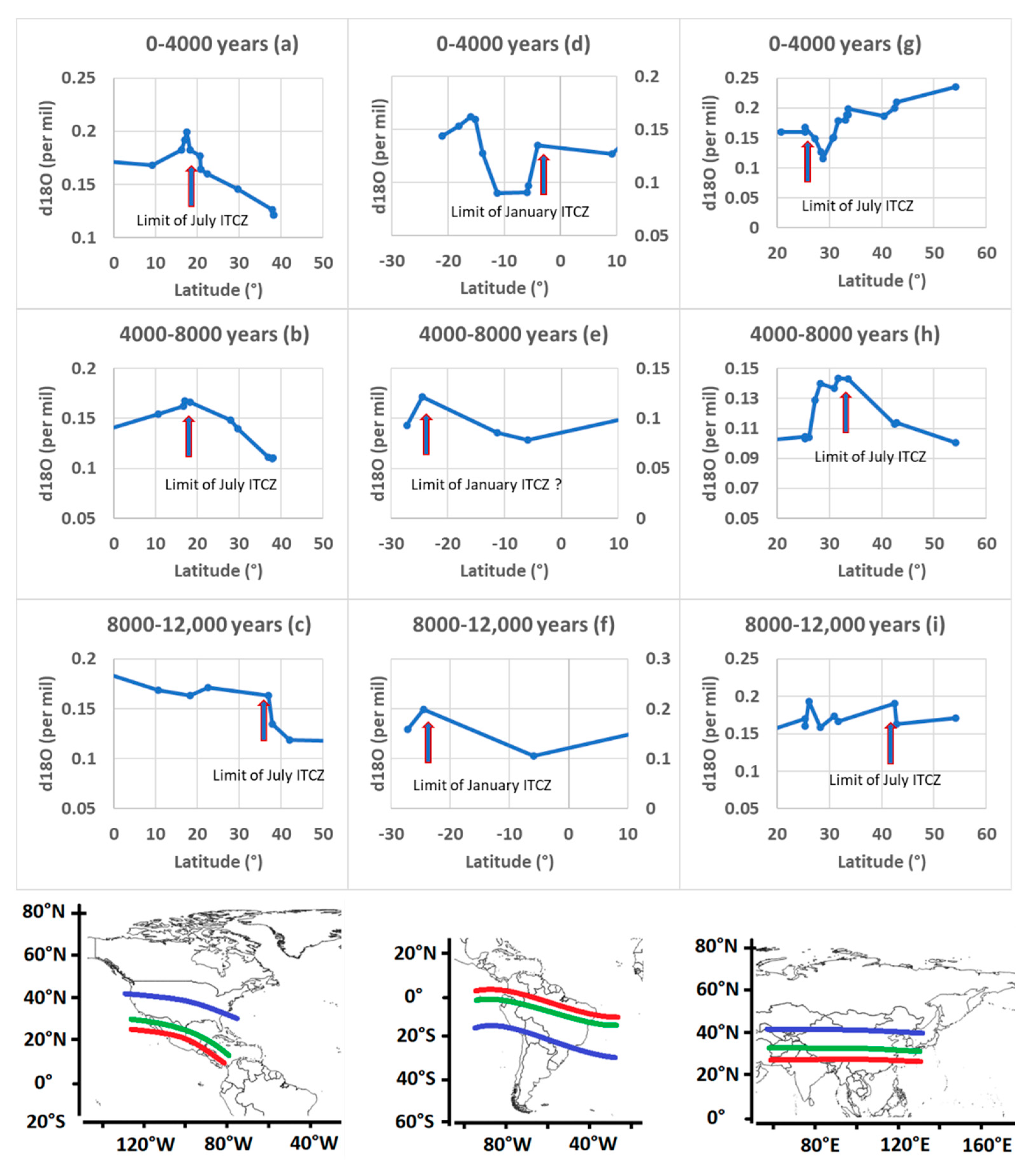
3.3. Variations in δ18O Concentration in Speleothems According to the Latitude
3.4. Variations in δ18O Concentration in Speleothems in the Tropical Pacific
4. Discussion
4.1. Decomposition in Subharmonic Modes
4.2. δ18O Concentration According to the Regions
4.2.1. Regions Located Outside the Hadley Cell
4.2.2. Regions Located Close to the Hadley Cell
4.3. The Atlantic Multidecadal Oscillation and the Subharmonic Mode
4.4. Latitudinal Shift of the Summer Intertropical Convergence Zone
4.5. Evolution of ENSO Activity during the Holocene
5. Conclusions
Author Contributions
Funding
Institutional Review Board Statement
Informed Consent Statement
Data Availability Statement
Acknowledgments
Conflicts of Interest
References
- Sadekov, A.Y.; Ganeshram, R.S.; Pichevin, L.; Berdin, R.; McClymont, E.; Elderfield, H.; Tudhope, A.W. Palaeoclimate reconstructions reveal a strong link between El Niño-Southern Oscillation and Tropical Pacific mean state. Nat. Commun. 2013, 4, 2692. [Google Scholar] [CrossRef] [Green Version]
- Barr, C.; Tibby, J.; Leng, M.J.; Tyler, J.; Henderson, A.C.G.; Overpeck, J.T.; Simpson, G.L.; Cole, J.E.; Phipps, S.J.; Marshall, J.C.; et al. Holocene El Niño–Southern Oscillation variability reflected in subtropical Australian precipitation. Sci. Rep. 2019, 9, 1627. [Google Scholar] [CrossRef]
- Qian, J. Multi-scale climate processes and rainfall variability in Sumatra and Malay Peninsula associated with ENSO in boreal fall and winter. Int. J. Clim. 2019, 40, 4171–4188. [Google Scholar] [CrossRef]
- Porter, S.E.; Mosley-Thompson, E.; Thompson, L.G.; Wilson, A.B. Reconstructing an Interdecadal Pacific Oscillation Index from a Pacific Basin–Wide Collection of Ice Core Records. J. Clim. 2021, 34, 3839–3852. [Google Scholar] [CrossRef]
- Reißig, S.; Nürnberg, D.; Bahr, A.; Poggemann, D.; Hoffmann, J. Southward Displacement of the North Atlantic Subtropical Gyre Circulation System During North Atlantic Cold Spells. Paleoceanogr. Paleoclimatol. 2019, 34, 866–885. [Google Scholar] [CrossRef]
- Pinault, J.-L. Long Wave Resonance in Tropical Oceans and Implications on Climate: The Pacific Ocean. Pure Appl. Geophys. Pageoph 2016, 173, 2119–2145. [Google Scholar] [CrossRef]
- Pinault, J.-L. Anticipation of ENSO: What teach us the resonantly forced baroclinic waves. Geophys. Astrophys. Fluid Dyn. 2016, 110, 518–528. [Google Scholar] [CrossRef]
- Pinault, J.-L. The Anticipation of the ENSO: What Resonantly Forced Baroclinic Waves Can Teach Us (Part II). J. Mar. Sci. Eng. 2018, 6, 63. [Google Scholar] [CrossRef] [Green Version]
- Pinault, J.-L. Regions Subject to Rainfall Oscillation in the 5–10 Year Band. Climate 2018, 6, 2. [Google Scholar] [CrossRef] [Green Version]
- Deininger, M.; McDermott, F.; Cruz, F.W.; Bernal, J.P.; Mudelsee, M.; Vonhof, H.; Millo, C.; Spötl, C.; Treble, P.C.; Pickering, R.; et al. Inter-hemispheric synchroneity of Holocene precipitation anomalies controlled by Earth’s latitudinal insolation gradients. Nat. Commun. 2020, 11, 5447. [Google Scholar] [CrossRef] [PubMed]
- Brahim, Y.A.; Wassenburg, J.A.; Cruz, F.; Sifeddine, A.; Scholz, D.; Bouchaou, L.; Dassie, E.; Jochum, K.P.; Edwards, R.L.; Cheng, H. Multi-decadal to centennial hydro-climate variability and linkage to solar forcing in the Western Mediterranean during the last 1000 years. Sci. Rep. 2018, 8, 17446. [Google Scholar] [CrossRef] [PubMed]
- Novello, V.F.; Vuille, M.; Cruz, F.; Stríkis, N.M.; de Paula, M.S.; Edwards, R.L.; Cheng, H.; Karmann, I.; Jaqueto, P.; Trindade, R.; et al. Centennial-scale solar forcing of the South American Monsoon System recorded in stalagmites. Sci. Rep. 2016, 6, 24762. [Google Scholar] [CrossRef] [PubMed]
- Pinault, J.-L. Resonantly Forced Baroclinic Waves in the Oceans: Subharmonic Modes. J. Mar. Sci. Eng. 2018, 6, 78. [Google Scholar] [CrossRef] [Green Version]
- Pinault, J.-L. Resonant Forcing of the Climate System in Subharmonic Modes. J. Mar. Sci. Eng. 2020, 8, 60. [Google Scholar] [CrossRef] [Green Version]
- Pinault, J.-L. Resonantly Forced Baroclinic Waves in the Oceans: A New Approach to Climate Variability. J. Mar. Sci. Eng. 2020, 9, 13. [Google Scholar] [CrossRef]
- Dansgaard, W. Stable isotopes in precipitation. Tellus 1964, 16, 438–468. [Google Scholar] [CrossRef]
- Rozanski, K.; Araguás-Araguás, L.; Gonfiantini, R. Isotopic patterns in modern global precipitation. In Climate Change in Continental Isotopic Records; Swart, P.K., Lohmann, K.L., McKenzie, J., Savin, S., Eds.; American Geophysical Union: Washington, DC, USA, 1993; pp. 1–37. [Google Scholar]
- Bony, S.; Risi, C.; Vimeux, F. Influence of convective processes on the isotopic composition (δ18O andδD) of precipitation and water vapor in the tropics: 1. Radiative-convective equilibrium and Tropical Ocean–Global Atmosphere–Coupled Ocean-Atmosphere Response Experiment (TOGA-COARE) simulations. J. Geophys. Res. Space Phys. 2008, 113, 19305. [Google Scholar] [CrossRef]
- Risi, C.; Bony, S.; Vimeux, F. Influence of convective processes on the isotopic composition (δ18O andδD) of precipitation and water vapor in the tropics: 2. Physical interpretation of the amount effect. J. Geophys. Res. Space Phys. 2008, 113, 19306. [Google Scholar] [CrossRef]
- Lachniet, M.S. Climatic and environmental controls on speleothem oxygen-isotope values. Quat. Sci. Rev. 2009, 28, 412–432. [Google Scholar] [CrossRef]
- Lachniet, M.S.; Patterson, W.P. Use of correlation and multiple stepwise regression to evaluate the climatic controls on the stable isotope values of Panamanian surface waters. J. Hydrol. 2006, 324, 115–140. [Google Scholar] [CrossRef]
- Li, G.; Cheng, L.; Zhu, J.; Trenberth, K.E.; Mann, M.E.; Abraham, J.P. Increasing ocean stratification over the past half-century. Nat. Clim. Chang. 2020, 10, 1116–1123. [Google Scholar] [CrossRef]
- Comas-Bru, L.; Atsawawaranunt, K.; Harrison, S.; SISAL Working Group Members. SISAL (Speleothem Isotopes Synthesis and AnaLysis Working Group) Database Version 2.0.; Dataset; University of Reading: Reading, UK, 2020. [Google Scholar] [CrossRef]
- GRIP Members. Climate Instability during the Last Interglacial Period Recorded in the GRIP Ice Core. Nature 1993, 364, 203–207. Available online: https://www.ncei.noaa.gov/pub/data/paleo/icecore/greenland/summit/grip/isotopes/gripd18o.txt (accessed on 5 August 2021). [CrossRef]
- Torrence, C.; Compo, G.P. A Practical Guide to Wavelet Analysis. Bull. Am. Meteorol. Soc. 1998, 79, 61–78. [Google Scholar] [CrossRef] [Green Version]
- Fohlmeister, J.; Vollweiler, N.; Spötl, C.; Mangini, A. COMNISPA II: Update of a mid-European isotope climate record, 11 ka to present. Holocene 2012, 23, 749–754. [Google Scholar] [CrossRef]
- Burns, S.J. A 780-year annually resolved record of Indian Ocean monsoon precipitation from a speleothem from south Oman. J. Geophys. Res. 2002, 107, ACL-9. Available online: https://agupubs.onlinelibrary.wiley.com/doi/full/10.1029/2001JD001281 (accessed on 5 August 2021). [CrossRef] [Green Version]
- Chen, S.; Hoffmann, S.S.; Lund, D.C.; Cobb, K.M.; Emile-Geay, J.; Adkins, J.F. A high-resolution speleothem record of western equatorial Pacific rainfall: Implications for Holocene ENSO evolution. Earth Planet. Sci. Lett. 2016, 442, 61–71. [Google Scholar] [CrossRef] [Green Version]
- Liu, X.; Guo, Q.; Guo, Z.; Yin, Z.-Y.; Dong, B.; Smith, R. Where were the monsoon regions and arid zones in Asia prior to the Tibetan Plateau uplift? Natl. Sci. Rev. 2015, 2, 403–416. [Google Scholar] [CrossRef]
- Partin, J.W.; Quinn, T.M.; Shen, C.-C.; Emile-Geay, J.; Taylor, F.W.; Maupin, C.R.; Lin, K.; Jackson, C.; Banner, J.L.; Sinclair, D.J.; et al. Multidecadal rainfall variability in South Pacific Convergence Zone as revealed by stalagmite geochemistry. Geology 2013, 41, 1143–1146. [Google Scholar] [CrossRef] [Green Version]
- Kennett, D.J.; Breitenbach, S.F.M.; Aquino, V.V.; Asmerom, Y.; Awe, J.; Baldini, J.U.; Bartlein, P.; Culleton, B.J.; Ebert, C.; Jazwa, C.; et al. Development and Disintegration of Maya Political Systems in Response to Climate Change. Science 2012, 338, 788–791. [Google Scholar] [CrossRef] [Green Version]
- Maupin, C.R.; Partin, J.W.; Shen, C.-C.; Quinn, T.M.; Lin, K.; Taylor, F.W.; Banner, J.L.; Thirumalai, K.; Sinclair, D.J. Persistent decadal-scale rainfall variability in the tropical South Pacific Convergence Zone through the past six centuries. Clim. Past 2014, 10, 1319–1332. [Google Scholar] [CrossRef] [Green Version]
- Winter, A.; Zanchettin, D.; Miller, T.; Kushnir, Y.; Black, D.; Lohmann, G.; Burnett, A.; Haug, G.H.; Estrella-Martínez, J.; Breitenbach, S.F.M.; et al. Persistent drying in the tropics linked to natural forcing. Nat. Commun. 2015, 6, 7627. [Google Scholar] [CrossRef] [PubMed]
- Pinault, J.-L. Modulated Response of Subtropical Gyres: Positive Feedback Loop, Subharmonic Modes, Resonant Solar and Orbital Forcing. J. Mar. Sci. Eng. 2018, 6, 107. [Google Scholar] [CrossRef] [Green Version]
- van Hengstum, P.; Donnelly, J.P.; Fall, P.L.; Toomey, M.R.; Albury, N.A.; Kakuk, B. The intertropical convergence zone modulates intense hurricane strikes on the western North Atlantic margin. Sci. Rep. 2016, 6, 21728. [Google Scholar] [CrossRef] [PubMed]
- Arbuszewski, J.A.; Demenocal, P.; Cléroux, C.; Bradtmiller, L.; Mix, A. Meridional shifts of the Atlantic intertropical convergence zone since the Last Glacial Maximum. Nat. Geosci. 2013, 6, 959–962. [Google Scholar] [CrossRef]
- Knudsen, M.F.; Seidenkrantz, M.-S.; Jacobsen, B.H.; Kuijpers, A. Tracking the Atlantic Multidecadal Oscillation through the last 8,000 years. Nat. Commun. 2011, 2, 178. [Google Scholar] [CrossRef]
- Haug, G.H.; Hughen, K.A.; Sigman, D.M.; Peterson, L.C.; Röhl, U. Southward Migration of the Intertropical Convergence Zone Through the Holocene. Science 2001, 293, 1304–1308. [Google Scholar] [CrossRef]
- Chiang, J.C.H.; Bitz, C.M. Influence of high latitude ice cover on the marine Intertropical Convergence Zone. Clim. Dyn. 2005, 25, 477–496. [Google Scholar] [CrossRef]
- Donohoe, A.; Marshall, J.; Ferreira, D.; McGee, D. The relationship between ITCZ location and cross equatorial atmospheric heat transport; from the seasonal cycle to the Last Glacial Maximum. J. Clim. 2013, 26, 3597–3618. [Google Scholar] [CrossRef]
- Collins, J.A.; Schefuß, E.; Heslop, D.; Mulitza, S.; Prange, M.; Zabel, M.; Tjallingii, R.; Dokken, T.M.; Huang, E.; Mackensen, A.; et al. Interhemispheric symmetry of the tropical African rainbelt over the past 23,000 years. Nat. Geosci. 2010, 4, 42–45. [Google Scholar] [CrossRef]
- Baker, P.A.; Seltzer, G.O.; Fritz, S.C.; Dunbar, R.B.; Grove, M.J.; Tapia, P.M.; Cross, S.L.; Rowe, H.D.; Broda, J.P. The History of South American Tropical Precipitation for the Past 25,000 Years. Science 2001, 291, 640–643. [Google Scholar] [CrossRef] [PubMed] [Green Version]
- Chiang, J.C.H.; Biasutti, M.; Battisti, D.S. Sensitivity of the Atlantic Intertropical Convergence Zone to Last Glacial Maximum boundary conditions. Paleoceanography 2003, 18, 1094. [Google Scholar] [CrossRef] [Green Version]
- Schmidt, M.W.; Spero, H.J. Meridional shifts in the marine ITCZ and the tropical hydrologic cycle over the last three glacial cycles. Paleoceanography 2011, 26, 1206. [Google Scholar] [CrossRef]


| Period (years) | Time (years) | Europe | Asia | Southeast Asia | New Zealand | North America | Central America | South America | ||||||||||||||
|---|---|---|---|---|---|---|---|---|---|---|---|---|---|---|---|---|---|---|---|---|---|---|
| M. | S.D. | N | M. | S.D. | N | M. | S.D. | N | M. | S.D. | N | M. | S.D. | N | M. | S.D. | N | M. | S.D. | N | ||
| 64 | 2000 | 0.11 | 0.01 | 20 | 0.14 | 0.02 | 31 | 0.07 | 0.01 | 6 | 0.15 | 1 | 0.13 | 0.03 | 2 | 0.14 | 0.02 | 11 | 0.14 | 0.01 | 25 | |
| 6000 | 0.12 | 0.02 | 14 | 0.13 | 0.02 | 19 | 0.08 | 1 | 0.12 | 1 | 0.15 | 0.03 | 4 | 0.12 | 0.04 | 8 | ||||||
| 10,000 | 0.12 | 0.02 | 7 | 0.15 | 0.03 | 13 | 0.07 | 1 | 0.14 | 0.05 | 2 | 0.12 | 0.03 | 3 | ||||||||
| 128 | 2000 | 0.11 | 0.01 | 27 | 0.14 | 0.02 | 35 | 0.06 | 0.00 | 5 | 0.15 | 1 | 0.11 | 0.03 | 4 | 0.14 | 0.02 | 10 | 0.13 | 0.01 | 21 | |
| 6000 | 0.10 | 0.01 | 20 | 0.12 | 0.01 | 25 | 0.07 | 1 | 0.10 | 0.01 | 3 | 0.15 | 0.03 | 5 | 0.10 | 0.01 | 7 | |||||
| 10,000 | 0.14 | 0.02 | 10 | 0.15 | 0.02 | 16 | 0.07 | 1 | 0.13 | 0.03 | 4 | 0.18 | 0.03 | 3 | 0.12 | 0.03 | 3 | |||||
| 256 | 2000 | 0.14 | 0.01 | 27 | 0.16 | 0.02 | 25 | 0.09 | 0.00 | 9 | 0.12 | 0.04 | 2 | 0.12 | 0.02 | 4 | 0.18 | 0.02 | 9 | 0.15 | 0.01 | 11 |
| 6000 | 0.11 | 0.01 | 21 | 0.16 | 0.02 | 23 | 0.08 | 0.01 | 7 | 0.11 | 1 | 0.11 | 0.02 | 5 | 0.19 | 0.03 | 6 | 0.13 | 0.01 | 10 | ||
| 10,000 | 0.18 | 0.01 | 12 | 0.20 | 0.02 | 18 | 0.09 | 0.01 | 8 | 0.17 | 1 | 0.15 | 0.02 | 4 | 0.20 | 0.01 | 3 | 0.16 | 0.04 | 5 | ||
| 768 | 2000 | 0.09 | 0.01 | 24 | 0.14 | 0.02 | 13 | 0.07 | 0.01 | 7 | 0.05 | 0.01 | 2 | 0.11 | 0.03 | 4 | 0.13 | 0.01 | 4 | 0.10 | 0.01 | 7 |
| 6000 | 0.09 | 0.01 | 21 | 0.15 | 0.02 | 20 | 0.06 | 0.01 | 6 | 0.05 | 0.02 | 2 | 0.09 | 0.03 | 4 | 0.11 | 0.02 | 6 | 0.10 | 0.01 | 11 | |
| 10,000 | 0.13 | 0.01 | 15 | 0.16 | 0.02 | 19 | 0.09 | 0.01 | 8 | 0.08 | 1 | 0.15 | 0.03 | 3 | 0.24 | 0.05 | 4 | 0.12 | 0.02 | 6 | ||
| 1536 | 2000 | 0.09 | 0.01 | 13 | 0.11 | 0.02 | 9 | 0.09 | 0.02 | 4 | 0.07 | 0.01 | 5 | 0.09 | 0.02 | 2 | 0.17 | 0.06 | 2 | 0.08 | 0.01 | 4 |
| 6000 | 0.09 | 0.01 | 14 | 0.12 | 0.01 | 13 | 0.08 | 0.02 | 5 | 0.08 | 0.01 | 6 | 0.16 | 0.08 | 2 | 0.16 | 0.07 | 3 | 0.11 | 0.02 | 5 | |
| 10,000 | 0.10 | 0.01 | 10 | 0.18 | 0.03 | 8 | 0.13 | 0.02 | 5 | 0.07 | 0.01 | 5 | 0.22 | 1 | 0.36 | 1 | 0.15 | 0.03 | 3 | |||
Publisher’s Note: MDPI stays neutral with regard to jurisdictional claims in published maps and institutional affiliations. |
© 2021 by the authors. Licensee MDPI, Basel, Switzerland. This article is an open access article distributed under the terms and conditions of the Creative Commons Attribution (CC BY) license (https://creativecommons.org/licenses/by/4.0/).
Share and Cite
Pinault, J.-L.; Pereira, L. What Speleothems Tell Us about Long-Term Rainfall Oscillation throughout the Holocene on a Planetary Scale. J. Mar. Sci. Eng. 2021, 9, 853. https://doi.org/10.3390/jmse9080853
Pinault J-L, Pereira L. What Speleothems Tell Us about Long-Term Rainfall Oscillation throughout the Holocene on a Planetary Scale. Journal of Marine Science and Engineering. 2021; 9(8):853. https://doi.org/10.3390/jmse9080853
Chicago/Turabian StylePinault, Jean-Louis, and Ligia Pereira. 2021. "What Speleothems Tell Us about Long-Term Rainfall Oscillation throughout the Holocene on a Planetary Scale" Journal of Marine Science and Engineering 9, no. 8: 853. https://doi.org/10.3390/jmse9080853
APA StylePinault, J.-L., & Pereira, L. (2021). What Speleothems Tell Us about Long-Term Rainfall Oscillation throughout the Holocene on a Planetary Scale. Journal of Marine Science and Engineering, 9(8), 853. https://doi.org/10.3390/jmse9080853