Application of Large Eddy Simulation to Predict Underwater Noise of Marine Propulsors. Part 2: Noise Generation

Abstract

Methods to predict underwater acoustics are gaining increased significance, as the propulsion industry is required to confirm noise spectrum limits, for instance in compliance with classification society rules. Propeller–ship interaction is a main contributing factor to the underwater noise emissions by a vessel, demanding improved methods for both hydrodynamic and high-quality noise prediction. Implicit large eddy simulation applying volume-of-fluid phase modeling with the Schnerr-Sauer cavitation model is confirmed to be a capable tool for propeller cavitation simulation in part 1. In this part, the near field sound pressure of the hydrodynamic solution of the finite volume method is examined. The sound level spectra for free-running propeller test cases and pressure pulses on the hull for propellers under behind ship conditions are compared with the experimental measurements. For a propeller-free running case with priory mesh refinement in regions of high vorticity to improve the tip vortex cavity representation, good agreement is reached with respect to the spectral signature. For behind ship cases without additional refinements, partial agreement was achieved for the incompressible hull pressure fluctuations. Thus, meshing strategies require improvements for this approach to be widely applicable in an industrial environment, especially for non-uniform propeller inflow.

1. Introduction

The rapid growth of shipping activities in the last century has created a substantial increase in anthropogenic noise in the oceans. The underwater background noise levels have intensified by up to $3 \mathrm{dB}$ per decade in specific frequency bands in some regions [1], which could be a source of deleterious effects on marine biology [2,3], especially when considering the comparatively short timescale of the transformation and the long lifespan of some species, such as cetaceans or testudines. In the frequency range from $10 \mathrm{Hz}$ to $300 \mathrm{Hz}$, the local underwater background noise level is elevated by $30 \mathrm{dB}$ when compared to the natural levels, according to some measurements. While further research is required to relate regional and seasonal dependencies as well as distinct frequency bands with their corresponding impact on individual marine species, regulatory institutions restrict overall noise levels in specific frequency ranges by using classification society guidelines that merely depend on the intended operational profile of the vessels [4].

1.1. State of the Art

The primary source of underwater radiated noise is the propeller [5,6], with tonal emissions at distinct blade passing frequencies, and its induced cavitation, generating broadband noise emissions caused by collapsing bubbles of various radii in sheet and tip vortex structures. Integrated behind a ship, the turbulence and cavitation is strongly affected by the non-uniform inflow, which creates unsteady vortex structures and fluctuating cavity regions with respect to a blade’s fixed coordinate system. Human comfort onboard is fundamentally affected by the spectral signature of the propellers, as near field acoustics are observed as pressure pulses on the vessel’s hull, which can be propagated across the vessel structure, if no precautions are undertaken with respect to the structural design of the vessel. In addition, underwater sound emission is a direct effect of the propeller’s operation in the vessel’s wake field and several interactions with the ship’s hull, as well as increased cavitation with higher vessel speeds, for which not all mechanisms are fully understood [7]. Contemporary propeller designs often purposefully allow for non-erosive cavitation patterns to reach higher efficiencies, which are primarily stable sheet cavitation fluctuating only with reductions in inflow velocity in the wake field and tip vortex cavitation, which is the main contributor to volume-based sound sources in the propeller slipstream [8].

Due to its current importance, there are numerous efforts to improve the quality of different types of numerical simulations to accurately predict all noise sources. Studies with boundary element methods (BEM) including the effects of a wake field show promising results regarding noise prediction caused by propeller cavitation in the near field [9] and far field by applying the Ffowcs Williams-Hawkings (FWH) acoustic analogy propagation method [10]. However, BEMs are based on reduced cavitation models and neglect viscosity, which certainly influences the slipstream evolution of the tip vortex cavity, and thus the volume-based acoustic sources. Accounting for sound sources caused by turbulent effects originating in the propeller slipstream may necessitate the use of volume-based methods, such as the finite volume method (FVM), rather than BEM.

Implicit large eddy simulation (ILES) turbulence modeling has been proposed for marine propeller simulations [11], and offers advantages with respect to solution speed and simplicity in handling. In part 1 of this study, adequately refined meshes and small time steps produce detailed cavitating tip-vortex flow for propeller free-running cases at model scale [12]. There, the PPTC’11 and Newcastle Round Robin propeller test case are investigated with feasible numerical effort for industrial application, although no hull is considered. In another investigation, the results of a propeller analysis with ILES in combination with the FWH method as a noise propagation tool were validated using the Newcastle and R/V Princess Royal test cases [13]. The inclusion of non-uniform inflow is one of the difficulties of propeller–hull interactions, as either the complete ship has to be modeled, or the induced velocities have to be imprinted onto the volume. Despite the operation conditions of the PPTC’15 test case being not closely application oriented, it serves as a demanding test case for cavitation and pressure pulse prediction methods, such as finite volume solvers. In the corresponding workshop [14], some good agreement was reached with respect to the cavitation structures on the blades; however, the prediction of pressure pulses was only fair, particularly in cavitating conditions. Another important application challenge is the interaction of rudders with the cavitating tip- or hub-vortices when integrated in a hull. Difficulties emerge at the interface between refined sliding meshes and, in the case of trailing vortex refinements, at the point of their intersection with the rudder. An adaptive mesh refinement strategy for the tip vortex was investigated in a study using the Newcastle test case [15], leading to the provision of highly detailed information regarding the cavity. In a further step, this approach was used by these authors to create an application-ready setup with inclusion of the hull [16].

Regarding noise emission, the influence of single bubbles and their oscillations and induced radiated pressure on the broadband noise signature was highlighted in a study with DES and the FWH method on a simple hydrofoil in a cavitation tunnel [17]. The power spectral density above $1 \mathrm{kHz}$ was affected significantly by the single bubble dynamics, which were implemented with several assumptions in the framework of a Euler-Lagrange coupling. These findings should be taken into account when considering the proposed approach here, which is purely Eulerian. Good agreement regarding the noise emissions of basic test cases with flow around cylinders was obtained with ILES in combination with the FWH method, where the control surface is on the cylinder surface [18]. A very recent study, which was similar to the present investigation, compared the Newcastle round robin test case acoustic emissions for one operation point with the respective measurements from the University of Genoa (UNIGE) cavitation tunnel. The results obtained with DES and the Schnerr-Sauer cavitation model reached good agreement regarding the underwater noise signature between 100 Hz and 10 kHz [19].

In the literature, there is some consensus that basic validation material with a sufficient quality and setup for the acoustic validation of numerical methods is still required, as model-scale tests are notoriously difficult to simulate with CFD with respect to acoustics due to basin or tunnel confinements, and are thus not ideal for developing a basic understand of the hydro-acoustic models. Full-scale testing, on the other hand, can be modeled as semi-infinite numerical domains, depending on the suitability of the trial location. However, propellers operate in a vessel’s wake, contributing with additional turbulent interaction, adding to the mix of indistinguishable broadband acoustic sources.

1.2. Contributions of Current Work

The acoustic evaluation of a marine propeller in the behind ship condition using CFD methods requires the accurate representation of all noise sources, in particular turbulence and cavitation, which require the resolution of low- and medium-wavelength turbulence. In this work, we report an industry-oriented feasibility study of an ILES-based numerical noise evaluation method, by analyzing the near-field acoustic emissions of two free-running propellers and their induced turbulence in the propeller slipstream, with one applying a vorticity-based a priori mesh refinement. The ability of the ILES approach to reproduce the spectral measurements is deemed sufficiently accurate for further studies of underwater acoustics. Subsequently, different proprietary propeller–hull combinations are studied in non-cavitating and cavitating flow at model and full scale. The main aspect of this study is the exploration of the limitations of the methods for resolving trailing vortices of propellers applied to practical cases of the propulsion industry. While the process works great for free-running propellers, the mesh refinement required for the cavitating tip vortex primarily prevents the use of the approach with more complex simulations, for instance, in the case of propellers in the behind ship condition, where appendages may obstruct the propeller slipstream.

2. Materials and Methods

The underlying physical models for hydrodynamic flow calculations, i.e., the treatment of turbulence, the two-phase flow mixture and the acoustic evaluation of the results, are listed. The models are implemented in OpenFOAM distribution, which is from Engys Ltd. and involves their HELYX versions 3.2.0 to 3.3.0. In the second part, the numerical setups for the Newcastle round robin test case and the P1595 propeller and propeller hull cases are presented.

2.1. Methodology

2.1.1. Hydrodynamics

Reynolds-Averaged-Navier-Stokes (RANS) equations are used throughout the study to initialize simulations or compare results, and are not described here, as they can be readily found in the literature. Based on successful studies regarding cavitating tip-vortex marine propeller flow with ILES in part 1 of this study [20], the implicit turbulence modeling approach without specific wall treatment is used for the acoustic evaluation. The conservation equations for a transient incompressible mixture $m$ in this case are

$$\frac{\partial {\rho }_m}{\partial t}+\frac{\partial \left({\rho }_m{\overline{u}}_i\right)}{\partial x_i}=0$$

(1)

$$\frac{\partial ({\rho }_m{\overline{u}}_i)}{\partial t}+\frac{\partial \left({\rho }_m{\overline{u}}_i{\overline{u}}_j\right)}{\partial x_i}=-\frac{\partial \overline{p}}{\partial x_i}+\frac{\partial }{\partial x_j}\left({\overline{S}}_{ij}-B_{ij}\right)+{\rho }_m{g}_i,$$

(2)

with the viscous stress tensor $S_{ij}=\mu \left(\frac{\partial u_i}{\partial x_j}+\frac{\partial u_j}{\partial x_i}\right)$, which utilizes the deformation rate tensor. For the sake of comparison, the Smagorinsky subgrid-scale model with a Van Driest damping function, enforced in the near-wall regions, is used for the P1595 free running case. In the cavitation simulations, only one set of transport equations is required for the water–vapor mixture, with an additional liquid phase fraction transport equation

$$\frac{\partial \alpha }{\partial t}+\nabla ·\left(\alpha u\right)+\nabla ·\left[u_c\cdot \alpha \left(1-\alpha \right)\right] = S_{\alpha },$$

(3)

where the source term is $S_{\alpha }=\frac{{\rho }_l}{{\rho }_l-{\rho }_v}{S}_m$ and $u_c$ is the artificial compression velocity field at the interface. The Schnerr-Sauer cavitation model, which is derived from the linearized Rayleigh-Plesset equation, is selected to model the mass transfer due to its stability and because it requires the least amount of unknown input from the experiments. The mass transfer between the phases is a function of the saturation pressure $p_V$, which can be assumed to be fixed for one experiment, and the local static pressure of the mixture $p$

$${\dot{m}}^{+}=C_V\left(1+{\alpha }_{Nuc}-\alpha \right)\frac{3{\rho }_L{\rho }_V}{\rho R}\sqrt{\frac{2}{3{\rho }_L}}\sqrt{\frac{1}{\left|p-p_V\right|}}\min \left(p-p_V,0\right),$$

(4)

$${\dot{m}}^{-}=C_c\alpha \frac{3{\rho }_L{\rho }_V}{\rho R}\sqrt{\frac{2}{3{\rho }_L}}\sqrt{\frac{1}{\left|p-p_V\right|}}\max \left(p-p_V,0\right)$$

(5)

The coefficients $C_V$ and $C_C$ for the vaporization and the condensation, respectively, are unity in the Schnerr-Sauer model. The model’s bubble radius

$$R=\sqrt[3]{ \frac{3\left(1+{\alpha }_{Nuc}-\alpha \right)}{4\pi n_0\alpha }}$$

(6)

is obtained from

$${\alpha }_{Nuc}=\frac{V_{Nuc}}{1+V_{Nuc}},$$

(7)

which is the nucleation volume fraction, where the nucleation volume is $V_{Nuc}=\frac{\pi n_0{d}_{Nuc}{}^3}{6}$. The remaining input parameters for the model are the nucleus density $n_0$ and the initial nucleus diameter $d_{Nuc}$, with the values listed in

Table 1. Parameters of the Schnerr-Sauer cavitation model.

Parameter	${\mathit{n}}_0$	${\mathit{d}}_{\mathit{N}\mathit{u}\mathit{c}}$
Unit	$1/m^3$	$m$
Value	$1\cdot {10}^{12}$	$1\cdot {10}^{-4}$

. They are selected as a compromise between stable cavitation structures and level of detail of trailing vortices, as demonstrated in a study with a hydrofoil [21].

The simulations apply a PIMPLE algorithm with a minimum of three outer corrector loops and three internal pressure corrector loops. Additional correctors and sub-cycles for the phase fraction equation are activated manually depending on the actual stability of the solution, which greatly affects the solver speed.

2.1.2. Acoustic Post-Processing

The sampling frequency is identical to the hydrodynamic simulation time step, with $\mathsf{\Delta }t=0.1°$, resulting in a Nyquist frequency of $63 \mathrm{kHz}$ in the case of the Newcastle model-scale propeller. The P1595 model propeller pressure spectra, obtained with a Hanning window and an energy correction factor, are compared with the experimental raw data in dB with respect to $p_{ref}$, with a Nyquist frequency of $54 \mathrm{kHz}$. For all simulations in which acoustic evaluations are carried out, the data collection commences once the forces and moments, as well as the vorticity and cavitation structures, in the propeller slipstream have converged. The acoustic pressure is reported over five total propeller revolutions in order to obtain sufficient data points in the frequency domain transformed signal.

In the behind hull condition, the near-field pressure pulse investigations use a time domain signal, which is subjected to a detrend function and a simple smoothing algorithm, before being transformed without window and correction factors. While the full-scale calculation applies no correction, the model-scale calculations are scaled with

$$p_s=p_m\cdot \frac{{\rho }_s{n}_s^2{D}_s^2}{{\rho }_m{n}_m^2{D}_m^2},$$

(8)

where the subscripts $m$ and $s$ indicate model and full scale, respectively, and $p$ is the pressure, $\rho$ the density, $n$ the rotation rate and $D$ the diameter. Due to the finite simulation time, the discrete data points require averaging at the harmonics of the blade passing frequency, indicated by the subscript $Harm$ in

$$p_{Harm,i}^{\prime }=\sqrt{{p^{\prime }}_{i-1}^2+{p^{\prime }}_i^2+{p^{\prime }}_{i+1}^2},$$

(9)

where $i$ signifies the integer index of the data points in the set.

Acoustic pressure time series of the Newcastle propeller round robin benchmark near-field results are processed in accordance with experimental reference [22], which in turn relies on the ITTC recommendations. The values obtained from the hydrodynamic solution are subjected to an FFT with a Hanning window applying an energy correction factor. In the frequency domain, a smoothing filter is applied to improve the semi-logarithmic representation of the results. With reference to the reference pressure $p_{ref}=1\cdot {10}^{-6} \mathrm{Pa}$ the sound pressure level (SPL) is obtained in $\mathrm{dB}$

$$SP{L}_m=10{\log }_{10}\left(\frac{{\overline{p}}^2}{p_{ref}^2}\right)$$

(10)

The results are compared to the experiments of the different participants in the Newcastle round robin benchmark at full scale, where the frequency is corrected with

$$f_s=f_m\frac{n_s}{n_m}\cdot \sqrt{\frac{{\sigma }_s}{{\sigma }_m}},$$

(11)

with the cavitation number being based on the rotation rate $\sigma$. The SPL amplitude is corrected with a constant shift of

$$SP{L}_s=SP{L}_m+20{\log }_{10}\left[{\left(\frac{{\sigma }_s}{{\sigma }_m}\right)}^{0.75}\left(\frac{r_m}{r_s}\right){\left(\frac{n_s{D}_s}{n_m{D}_m}\right)}^{1.5}{\left(\frac{D_s}{D_m}\right)}^{1.5}\right],$$

(12)

where $r_m$ is the distance of the simplified point sound source at the intersection of the propeller plane and the rotation axis and the observer and $r_s=1 \mathrm{m}$, according to the standard for underwater radiated noise. In this expression, constant bandwidth exponents are applied. Different from the reference, a transfer function is not used in the numerical simulation.

The FWH method is an inhomogeneous wave equation that is applicable to moving surfaces in free unlimited streams. The results of a variation of this acoustic analogy are used in one of the cases of the present study as a comparison to near-field pressure fluctuations from the hydrodynamic solution obtained from the underlying FVM. The FWH acoustic analogy distinguishes sources by types [23], with monopoles for the thickness $p{\prime }_T$, dipoles for the lifting forces $p{\prime }_L$, and quadrupoles for non-linear contributions $p{\prime }_Q$ in the volume

$$p^{\prime }\left(\overrightarrow{x},t^{\ast }\right)=p_T^{\prime }\left(\overrightarrow{x},t^{\ast }\right)+p_L^{\prime }\left(\overrightarrow{x},t^{\ast }\right)+p_Q^{\prime }\left(\overrightarrow{x},t^{\ast }\right).$$

(13)

Evaluation of the final term as a volume integral is expensive, and thus the permeable surface formulation of the FWH is used, where the sound sources are evaluated with a surface integral on a cylindrical control surface, aligned with the axis of propeller rotation. Since the volume-based acoustic sources creating the spectral contributions of interest are located in the trailing flow behind the propeller and as cavities on the blades, the control surface spans the regions of interest and evaluates the terms on the surface. Thereby, the terms surrender the original meanings of thickness and loading, making the evaluation of the volume integral inside the control surface closure obsolete. With the time derivatives as an input, the first two terms yield

$$p_T^{\prime }\left(\overrightarrow{x},t^{\ast }\right)=\frac{1}{4\pi }{{\displaystyle \int }}_S^{ }{\left[\frac{{\rho }_0\left(\dot{v_{\mathrm{n}}}+v_{\dot{n}}\right)}{r{\left(1-M_r\right)}^2 } \right]}_{ret}dS+\frac{1}{4\pi }{{\displaystyle \int }}_S^{ }{\left[\frac{{\rho }_0{v}_n\left(r{\dot{M}}_r+c{M}_r-c{M}^2\right)}{r^2{\left|1-M_r\right|}^3 } \right]}_{ret}dS$$

(14)

$$\begin{array}{c}{p}_L^{\prime }\left(\overrightarrow{x},t^{\ast }\right)=\frac{1}{4\pi c}{{\displaystyle \int }}_S^{ }{\left[\frac{{\dot{l}}_r}{r{\left(1-M_r\right)}^2 } \right]}_{ret}dS+\frac{1}{4\pi }{{\displaystyle \int }}_S^{ }{\left[\frac{l_r-l_M}{r^2{\left(1-M_r\right)}^2 } \right]}_{ret}dS+\\ \frac{1}{4\pi c}{{\displaystyle \int }}_S^{ }{\left[\frac{l_r\left(r{\dot{M}}_r+c{M}_r-c{M}^2\right)}{r^2{\left|1-M_r\right|}^3}\right]}_{ret}dS,\end{array}$$

(15)

with the dimensional notations omitted for clarity. The undisturbed density of the fluid is ${\rho }_0$, the distance from the sound source to the observer point at $\overrightarrow{x}$ is $\overrightarrow{r}$, the Mach number is $\overrightarrow{M}$ and $S$ is the body surface. The subscripts represent a dot product of the vector with the unit normal vector $\overrightarrow{n}$ on the surface into the fluid, its time derivative $\dot{\overrightarrow{n}}$, the unit radiation vector $\widehat{\overrightarrow{r}}$ or the surface velocity Mach number vector $\overrightarrow{M}$. In the permeable surface formulation, the terms for the relative velocity between the surface and the fluid $\overrightarrow{v}$ and the surface term $\overrightarrow{l}$ are

$$\overrightarrow{v}=\overrightarrow{V}+\frac{\rho }{{\rho }_0}\left(\overrightarrow{U}-\overrightarrow{V}\right),$$

(16)

$$\overrightarrow{l}=p\overrightarrow{n}+\rho \overrightarrow{U}\left(u_n-v_n\right),$$

(17)

where $\overrightarrow{U}$ is the fluid velocity and $\rho$ is the actual density of the fluid. Due to the attenuation properties, $r^{-2}$ terms are dominant in the near field and $r^{-1}$ terms in the far field. The surface is the emitting sound source, so the far-field sound pressure can be obtained even outside the hydrodynamic domain for the complete simulation duration. Due to the sound propagation velocity, the values at the observer are generated for the time of emission, by linearly interpolating the locations of the surface sources at the retarded time between two adjacent time steps $t_1\le t_{ret}\le t_2$ considering the distance from the source to the observer

$$t_{ret}=t^{\ast }-\frac{\left|\left|\overrightarrow{x}\left(t^{\ast }\right)-\overrightarrow{y}\left(t\right)\right|\right|}{c}$$

(18)

with $\overrightarrow{y}$ as the sound source point. The surface assumes the shape of a cylinder with closed end caps, where an offset of $1 \mathrm{m}\mathrm{m}$ mm is created outside the sliding mesh interface. The exact control surface extent and the effects of the cylinder bases have been discussed in the literature, specifically the fact that the end caps create additional spurious noise [24]. In the available implementation, the end caps are removable, and their influence, as well as the axial extent of the surface, should be studied in detail in the future. However, the mesh of the underlying hydrodynamic simulation determines the quality of the sound pressure obtained as input for the permeable surface and thus the acoustic results of such an investigation may be more susceptible to the numerical effects of the FVM or increase the numerical effort in the case of increased numbers of cells to counter these effects.

2.2. Numerical Setup

2.2.1. Free-Running Propellers

The Newcastle propeller test case is modeled in the round robin configuration of UNIGE with a diameter of $D_M=0.22 \mathrm{m}$ and a tunnel with a quadratic cross section with rounded edges and an area of around $A=0.32 {\mathrm{m}}^2$.

Table 2. Newcastle test case. Considered test conditions for the round robin test.

Condition	C1	C2	C3	C6
$J \left[-\right]$	$0.4$	$0.4$	$0.4$	$0.5$
${\sigma }_n \left[-\right]$	$2.22$	$1.3$	$0.72$	$1.13$
$n$ [Hz]	35	35	35	35

compiles the investigated conditions C1 to C3 and C6 [22], which present tip vortex cavitation to varying extents in pull configuration, and feature acoustic spectral measurements from six participating model test facilities. Geometric descriptions of the Newcastle propeller used at the different test facilities during the round robin tests are available in the literature.

The P1595 test case is another free-running propeller with $D_P=0.204 \mathrm{m}$, investigated as part of the ProNoVi research project in the SINTEF Ocean cavitation tunnel, with the geometric data listed in

Table 3. P1595. Main geometric data.

Parameter	Symbol	Unit	Value
Diameter	$\mathrm{D}$	$\left[\mathrm{mm}\right]$	$204$
Design pitch ratio	${\mathrm{P}}_{0.7\mathrm{R}}/\mathrm{D}$	$\left[-\right]$	$1.188$
Chord length at $r/R=0.7$	${\mathrm{C}}_{0.7\mathrm{R}}$	$\left[\mathrm{mm}\right]$	$79.132$
Max. thickness at $r/R=0.7$	${\mathrm{t}}_{0.7\mathrm{R}}$	$\left[\mathrm{mm}\right]$	$3.617$
Area ratio	${\mathrm{A}}_{\mathrm{E}}/{\mathrm{A}}_0$	$\left[-\right]$	$0.626$
Hub ratio	${\mathrm{d}}_{\mathrm{h}}/\mathrm{D}$	$\left[-\right]$	$0.196$
Skew-angle	$\mathsf{\Theta }$	$\left[°\right]$	$42$
Number of blades	$\mathrm{Z}$	$\left[-\right]$	$4$
Sense of rotation	-	$\left[-\right]$	$\mathrm{Right}$
Type of propeller	-	$\left[-\right]$	$\mathrm{FP} \left(\mathrm{Fixed} \mathrm{Propeller}\right)$

. It possesses a slightly more application-oriented cavitating tip and hub vortex appearance, and the test campaign features hydroacoustic measurements in free-running and behind-ship conditions. To further verify the proposed acoustic evaluation approach, a free-running operation point at $J=0.6$ in combination with a rotation rate of $n=30 \mathrm{Hz}$ is selected, with a cavitation number of ${\sigma }_n=1.5$.

The setups feature an inlet fixed to the respective velocity of the experiment and the outlet is set to the experimental pressure, which creates a uniform pressure independent of the gravity, which at model scale is a sufficiently close approximation of the experimental conditions. The remaining surfaces are set to no-slip walls for the Newcastle case and to slip walls for the P1595 case. The rotating region is defined as a cyclic arbitrary mesh interface (AMI).

Turbulent fluctuations are generated either based on shear in a boundary layer or by flow shear behind sharp edges of solid bodies, such as the trailing edge of the propeller, leading to the conclusion that the cavitating tip vortex is primarily influenced by the edge shear. Therefore, the premise of this study is that the acoustic emissions generated by cavitation and turbulence in the propeller slipstream are not highly dependent on the strict resolution of the law of the wall. While the law of the wall demands a high degree of near-wall mesh resolution for LES, for which different suggestions can be found in the literature, such as $y^{+}\le 2$, as well as $x^{+}\le 10$ and $z^{+}\le 5$ [25], where y is the wall orthogonal and x the streamwise direction, these are considered unfeasible for industrial use due to the highly inflated cell count and the corresponding numerical resource requirements. Thus, a reduction in the numerical effort required for LES would be highly favorable, and is of particular importance for acoustic evaluations, where fine time steps and high numbers of rotations are essential for spectral analyses. For the Newcastle case, the non-dimensionalized wall distance of the first cell is $y^{+}\approx 10$ on the propeller blades, which might negatively affect the force prediction, as no wall model is used. The P1595 study, on the other hand, employs a mesh wall resolution of $y^{+}<1$ everywhere on the blade.

The initial mesh in Figure 1a incorporates distance refinement on the suction side near the leading edges in order to resolve the sheet cavitation, an annulus refinement from $\frac{r}{R}\approx 0.68$ to $\frac{r}{R}\approx 1.10$ with an axial extent of $2\cdot D$ from the propeller plane for the tip vortex, and an additional refinement at the blade tips, in order to facilitate tip vortex development in the mixing zone. In the figure, the green dashed line indicates the sliding mesh interface, which also features increased refinement level compared to the surrounding mesh. A hub vortex, which is missing in the experiment due to the pulling configuration, is avoided by extending the shaft to the intersection with the domain outlet, reducing slipstream effects that might affect acoustics. For the P1595 study, a mesh is created, as shown in Figure 1b, with a quasi-infinite domain without tip or hub vortex refinements; however, the complete rotating region downstream of the propeller features a finer mesh, as a minor influence of the downstream refinement on the integral propeller forces and moments is detected. The shaft of this push configuration is extruded toward the inlet of the domain. All utilized meshes are listed in

Table 4. Size of initial mesh and examples of the applied refinements.

$\mathbf{Cell} \mathbf{Count} [{10}^6 \mathbf{Cells}]$
	Newcastle	P1595
Initial mesh	$13.0$	$13.1$
Refinement step	C1: $32.3$ C2: $24.9$ C3: $27.5$ C6: $40.1$	-

, with the respective a priory mesh refinement steps in the case of the Newcastle propeller.

On the initial meshes, the refinements are not sufficient to develop cavitating tip vortices, for which the sizes would increase to an unfeasible cell count with conventional meshing methods. Therefore, an a priori mesh refinement strategy based on vorticity is used in the Newcastle case as an intermediate step in order to resolve the tip vortex turbulence and cavity structures. In Figure 2, the vorticity isosurface at $Q=5\cdot {10}^5 {\mathrm{s}}^{-2}$ is extracted, which is used in a complete remeshing, where it is included as a source for a distance refinement. The cell size in the refinement region follows a minimum bubble diameter of $r_b=0.1\%\cdot D_P$, which is a value obtained experimentally [26].

The phase transition solver interPhaseChangeDyMFoam is based on the physical dynamic pressure definition, which means an initial steady state calculation to quickly achieve flow convergence is not attainable, as the available steady state solvers are based on the kinematic pressure definition. Instead, a transient precursor RANS simulation with time steps of $\mathsf{\Delta }t=1°$ is employed for 12 rotations, during which cavitation is suppressed by setting the saturation pressure to $p_{sat}=-1\cdot {10}^{10 }\mathrm{Pa}$. The ILES is then run for two rotations with a time step of $\mathsf{\Delta }t=0.1°$, and subsequently, the saturation pressure is gradually increased, while the environment pressure is constant, which itself takes about one rotation. Following this procedure, the cavitating part of the simulation is run for another two rotations. After the mesh refinement, another five rotations are calculated for the acoustic evaluation. Convergence is checked by monitoring the isosurfaces of the trailing vortex structures, i.e., the vorticity with $Q=5\cdot {10}^5$ over time, on the basis of videos. It is found that the integral forces and moments of the propeller converge before the trailing flow structures. Numerical equation residuals are not considered for monitoring as they usually converge before the integral values, especially for transient simulations.

2.2.2. Ship–Propeller Configurations

In this part, the methods are applied, under the constraints imposed by the more complex geometries, to near-field acoustic investigations in behind-ship condition for three confidential test cases. In Figure 3, the domains and the regions of interest near the propeller are highlighted in red in the mesh, with the sliding mesh interface indicated by a dashed green line. The positioning of the permeable FWH surface with respect to the sliding mesh interface is found to be ideal if it is $1 \mathrm{mm}$ larger than the sliding mesh interface in all directions. This condition is applied to behind-ship simulations that apply acoustic evaluations with the FWH method, which means in the figure, the sliding mesh interface possesses sufficient accuracy when it coincides with the green dashed line. All meshes apply a high Reynolds approach, with $y^{+}\ge 30$ on the propeller and the hull. Similar to the free-running propeller setups, a velocity inlet based on the ship advance ratio is applied. The constant pressure outlet is equal to the experimental conditions at model scale; at full scale, a pressure corresponding to the value at $r/R=0.7$ at the 12 o’clock blade position is set. The ProNoVi reference target case is a twin-screw yacht vessel with two conventional shaft lines, which is simulated in $\lambda =21.08$ scale with $D_M=2.04 \mathrm{m}$ at $k_T$ similarity of about $k_T\approx 0.20$ with respect to the propulsion. There are three shaft brackets and shaft fairings directly upstream of the propeller, which are expected to have a significant impact on the angular propeller loads and thus on noise generation. Full-scale corrected pressure pulse measurements in non-cavitating conditions with $J=0.74$ and $n=20.5 \mathrm{Hz}$ are compared to the experimentally obtained values for a semi-model with a tip clearance of about $0.31\cdot D_P$. Due to the counter-rotating shaft lines, a symmetry boundary condition is imposed at the vertical ship centerline, and the experimental setup reflects this through the no-slip condition for the cavitation tunnel walls. The downstream rotating mesh interface around the propeller is required to terminate between the propeller hubcap and the rudder, which means that the currently proposed tip vortex refinement process is unreasonable due to the non-axisymmetric geometry in the slipstream. Note the oblique flow conditions due to the shaftline inclination of $2.75°$, which is reflected by rotating the mesh and the gravity vector. With respect to the trailing vortex mesh refinements, the direction of flow is not immanently followed, although the refinements are generally wider in the radial direction to allow for trailing vortex drift with respect to the rotation axis of the rotating region.

As the first SCHOTTEL reference case, a $D_S=5.8 \mathrm{m}$ propeller container feeder with one horizontal conventional shaft line is investigated under cavitating conditions in full scale and compared to the scaled experimental measurement at $J=0.89$, $n=1.85 \mathrm{Hz}$ and with a cavitation number of ${\sigma }_{0.7}=1.87$ at $r/R=0.7$ in 12 o’clock position. From a precursor resistance calculation, the surface wave pattern is extracted and reused as the domain surface with a symmetry type boundary condition, while the remaining far field boundaries are declared to be walls. In this case, an acoustic evaluation is conducted using the permeable surface FWH method, where the control surface is placed directly outside of the rotating mesh region, meaning the rudder is not among the acoustic sources considered. The tip clearance in the full model is $0.25\cdot D_P$.

The second SCHOTTEL reference case is an azimuthing twin propeller booster drive for a yacht vessel located on the centerline at vessel stern, which is investigated at $\lambda =9.5$ model scale and compared to experimental model-scale measurements. An improved propeller design is then simulated again in order to demonstrate its reduced pressure pulse amplitudes on the hull. Symmetry conditions are prescribed for all far-field boundaries, as well as the water surface. For the propulsion unit with both propellers at $D_P=2.5 \mathrm{m}$, an advance coefficient of $J=1.07$ and a propeller speed of $n=17 \mathrm{Hz}$ are investigated, assuming a relatively high cavitation number of ${\sigma }_n=2.78$ and an average tip clearance of $0.58\cdot D_P$. This mesh has the highest cell count, as two propellers are simulated and the region between the propeller planes requires high mesh resolution, particularly at the tip vortex, in order to capture the turbulent interaction between the propellers and the housing structure, including the fins. Regarding the convergence monitoring of these cases, similar techniques are used to those described in Section 2.2.1.

3. Results

In the first part, the quality of the noise spectral results for the Newcastle benchmark test case and the P1595 propeller is assessed. In the second part, the behind hull cases are evaluated in model and full scale as pressure pulses on the hull.

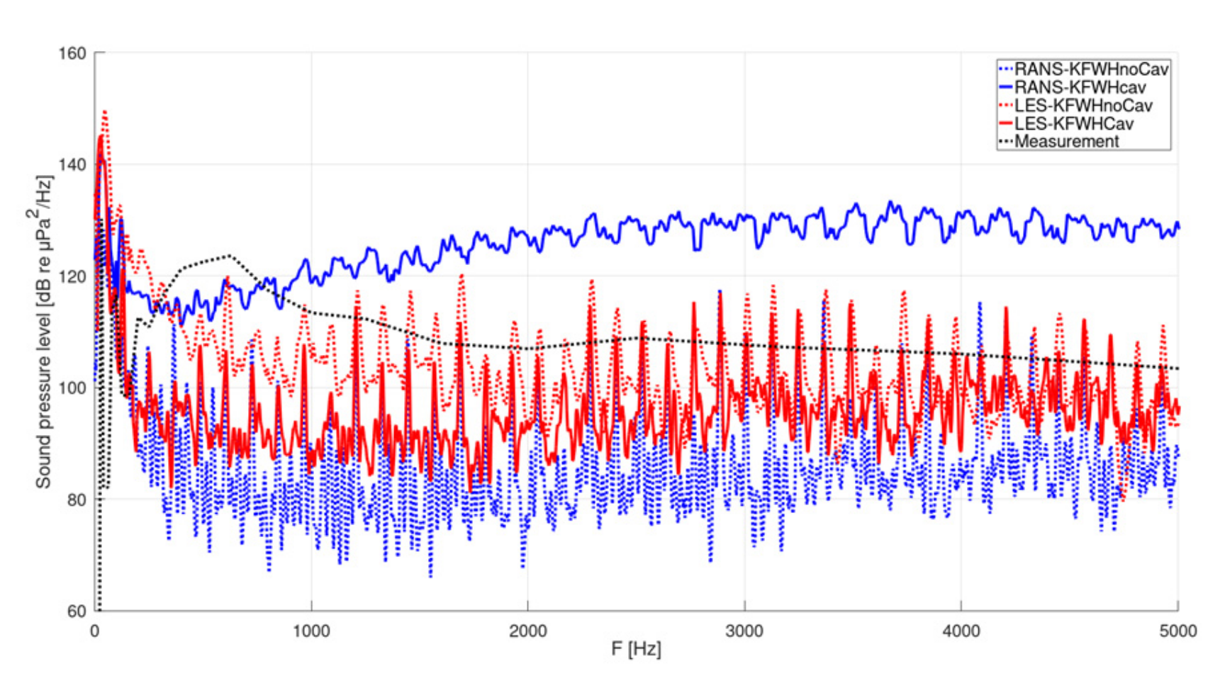
3.1. Radiated Noise Analysis

3.1.1. Newcastle Propeller Test Case

Figure 4 presents a comparison of the narrowband spectrum and one-third octave band measurements. The acoustic spectrum at the pressure observer H2, as illustrated in Figure 4a, confirms the proposed setup, as the distance between the prediction and measurement decreases with the increasing level of detail in the models in Figure 4b. Here the results are scaled to full scale and normalized according to the ITTC recommendation in the same way as in the experiment [27]. For reference, there is the round robin test measurements of UNIGE [22], while the same simulation was performed in a quasi-infinite domain by SINTEF Ocean, conducted with STAR-CCM+ and LES with a standard Smagorinsky subgrid-scale model in cavitating condition. A reduction of noise signals from the time-averaged RANS turbulence modeling to the ILES medium and large-scale turbulence modeling is to be expected, and the activation of the phase change (cavitation model) decreases the sound level by a further $15–20 \mathrm{dB}$ in the medium frequency range from $100 \mathrm{Hz}$ to $3 \mathrm{kHz}$, which is the opposite of the expected effects of increased underwater noise emission associated with cavitation. The application of the AMR technique, which is also indicated in the diagram, in the tip vortex region leads to a reduction of the high frequency pressure fluctuations by an additional $10 \mathrm{dB}$, leading to improved agreement with the measurements in the range above $3 \mathrm{kHz}$. A reason for the decreased SL with the activation of the phase change and the further reduction with the application of mesh refinement, and thus appearance of an extended cavitating tip vortex, could be that the cavitation is in this case attenuating the acoustic pressure, which appears as a stable water vapor region turning in complete synchronization with the propeller, and a bursting of the tip vortex is not observed. The stability in the simulation is also confirmed by the observations in part 1 of this study, where the modes of vibration proposed in [28] could not be detected. Inflow perturbations might be needed in the numerical simulation to create instability of the cavity, and thus noise. Similarly, single bubble contributions that detach from the sheet and tip vortex cavity are not considered in this approach, and they could also affect the behavior. Finally, the linearized Rayleigh-Plesset equation, which is the basis for the Schnerr-Sauer cavitation model, might be inadequate for predicting both the vibration modes and the associated effects of the acoustic emissions.

In Figure 5, the SL simulation results for all of the studied Newcastle conditions, for the three observers H1-3, are related to their corresponding measurements, as indicated by the dashed black line. In frequency ranges without measurement data, the UNIGE data points are connected linearly in the graph. In theory, due to the scaling process onto a distance of $r_{ref}=1 \mathrm{m}$, the observer results should be similar. A good agreement is reached at the lower and higher frequencies, except for condition C6 (Figure 5d). In particular, C1 (Figure 5a) and C6 fail to predict the medium frequency peak between 200 and 300 Hz by more than 20 dB, with C6 shifted up to 10 dB in the higher frequencies compared to the measurement, although the trend of the curve is correct. The green region indicates the envelope of all measurements taken in the Newcastle round robin test, which means that simulation results within these limits can be considered acceptable, when taking into account the margins of reproducibility dictated by high-end contemporary measurement technology.

3.1.2. P1595

Table 5. P1595: integral values at $J=0.6$.

Type	${\mathit{K}}_{\mathit{T}}$	$10 {\mathit{K}}_{\mathit{Q}}$	$\mathbf{\Delta }{\mathit{K}}_{\mathit{T}}$	$\mathbf{\Delta }10 {\mathit{K}}_{\mathit{Q}}$	$\Delta {\eta }_0$
Experiment (Cav Off)	0.305	0.536	-	-	-
Experiment (Cav On)	0.302	-	-	-	-
$\mathrm{RANS} \mathrm{k}-\mathsf{\omega }-\mathrm{SST} \mathrm{no} \mathrm{cavitation}$	$0.308$	$0.532$	$0.9\%$	$1.8\%$	$1.8\%$
$\mathrm{RANS} \mathrm{k}-\mathsf{\omega }-\mathrm{SST} \mathrm{cavitation}$	$0.297$	$0.537$	$-1.7\%$	$-$	$-$
$\mathrm{LES} \mathrm{Smagorinsky} \mathrm{no} \mathrm{cavitation}$	$0.309$	$0.541$	$1.3\%$	$0.4\%$	$0.4\%$

lists the predicted integral forces and moments for the P1595 propeller, which could be improved by increasing the number of PIMPLE outer correctors. Figure 6 illustrates the simulation setup as well as the visual comparison of the simulation results with the experimental observation regarding cavitation. In the simulation, an acoustic observer is placed at the same location as the hydrophone in the measurement. The cavitation region on the blade is predicted accurately, occurring only at the tip; however, the tip vortex, and in particular the clouds in the mixing zone, are not captured accurately, as a result of the unrefined mesh in this region. It is important to note that there is a thin developed tip vortex filament in addition to the trailing tip vortex cloud cavitation in the experiment for this operation condition.

The acoustic pressures obtained from the permeable surface FWH method (KFWH) are compared, as the sound pressure level with respect to $p_{ref}=1\cdot {10}^{-6 }\mathrm{Pa}$, with the measurement data from the experiment in Figure 7, which shows the spectral density plots. The first blade frequency at $f=120 \mathrm{Hz}$ creates a peak, which is prominent independent of the simulation approach. For the RANS results there is a significant difference between the non-cavitating and cavitating conditions in the medium and high frequencies; however, neither result is in agreement with the measurements, which are only available in cavitating condition. Active cavitation increases the sound pressure obtained from RANS beginning at $f\approx 120 \mathrm{Hz}$, from where an overpridiction of up to $20 \mathrm{dB}$ occurs over all frequency ranges. With LES, the sound pressure level is increased by about $10 \mathrm{dB}$ over most of the medium and high frequencies compared to the non-cavitating RANS simulation, leading to better agreement with the measurement, confirming the necessity to resolve turbulent length scales in the acoustic simulations. Similar to what was observed with the Newcastle simulations, the activation of cavitation for LES leads to a reduction of the sound pressure amplitudes over the displayed frequency range of about $5–10 \mathrm{dB}$. It is expected that the cavitating tip vortex and the observed bursting increases the sound pressure level in this case, leading to inaccuracies in the prediction, confirming that the mesh refinement is required for acoustic predictions.

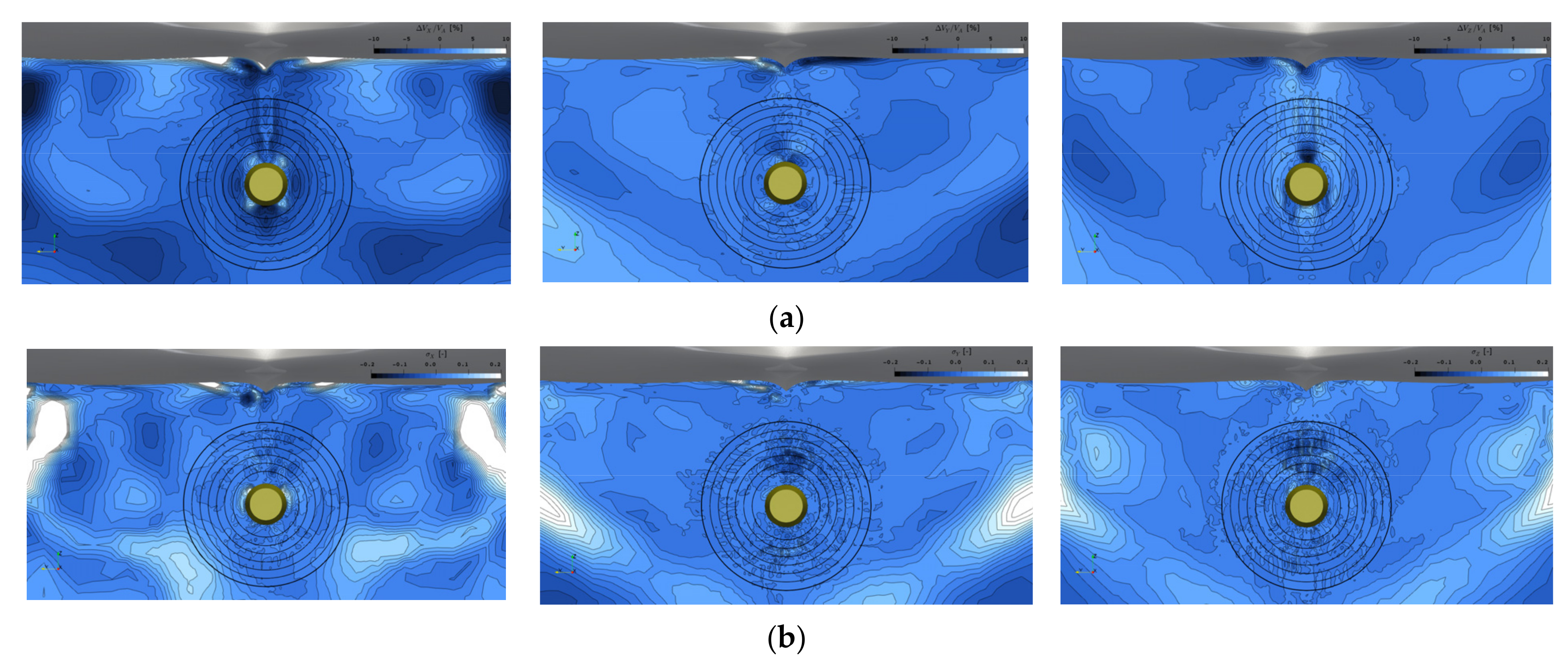
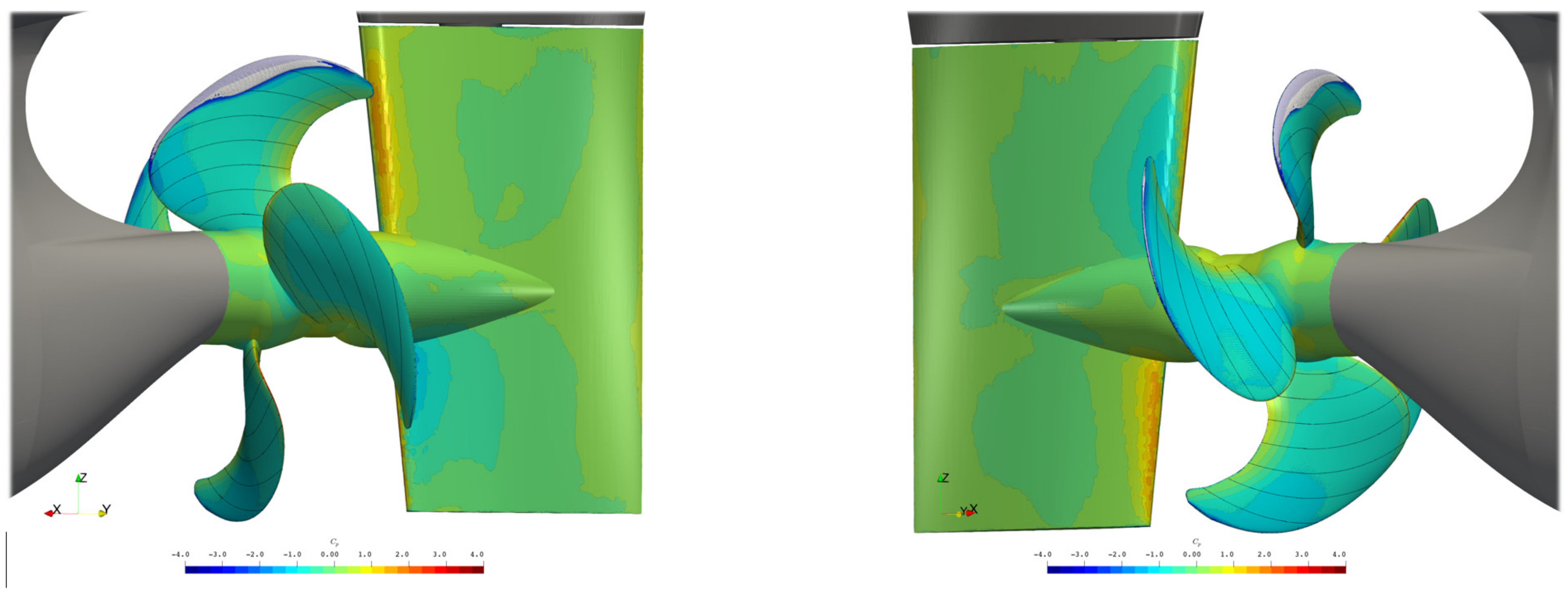
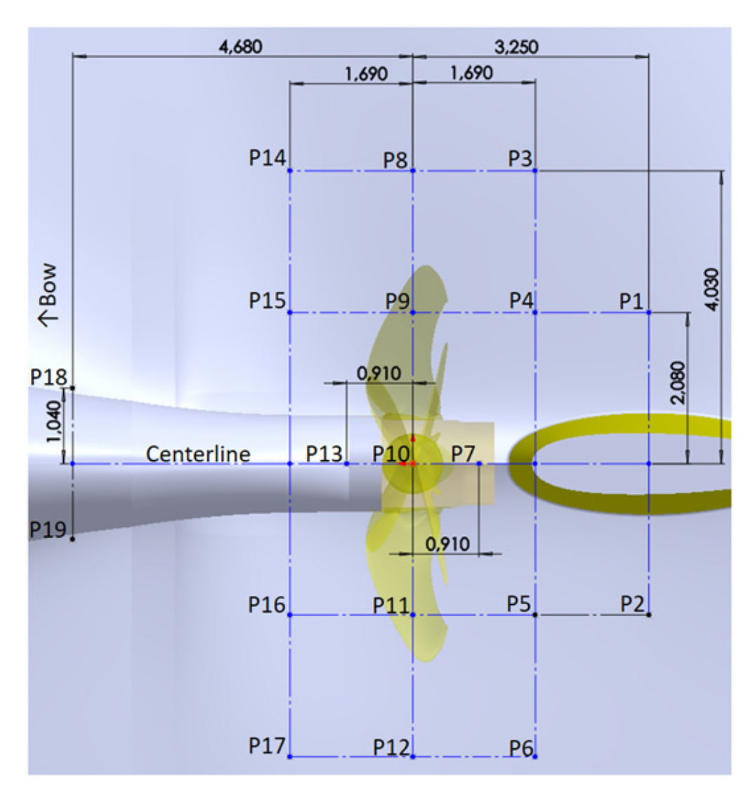
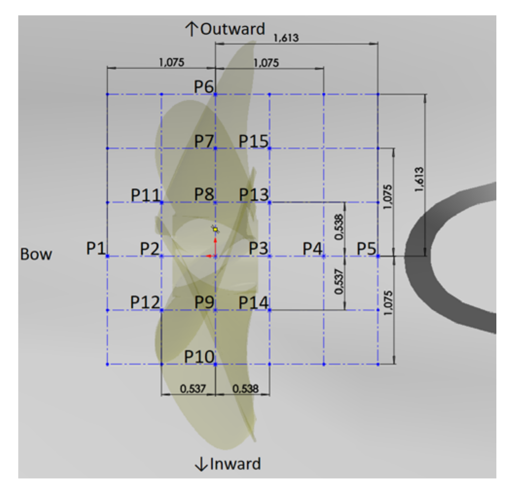
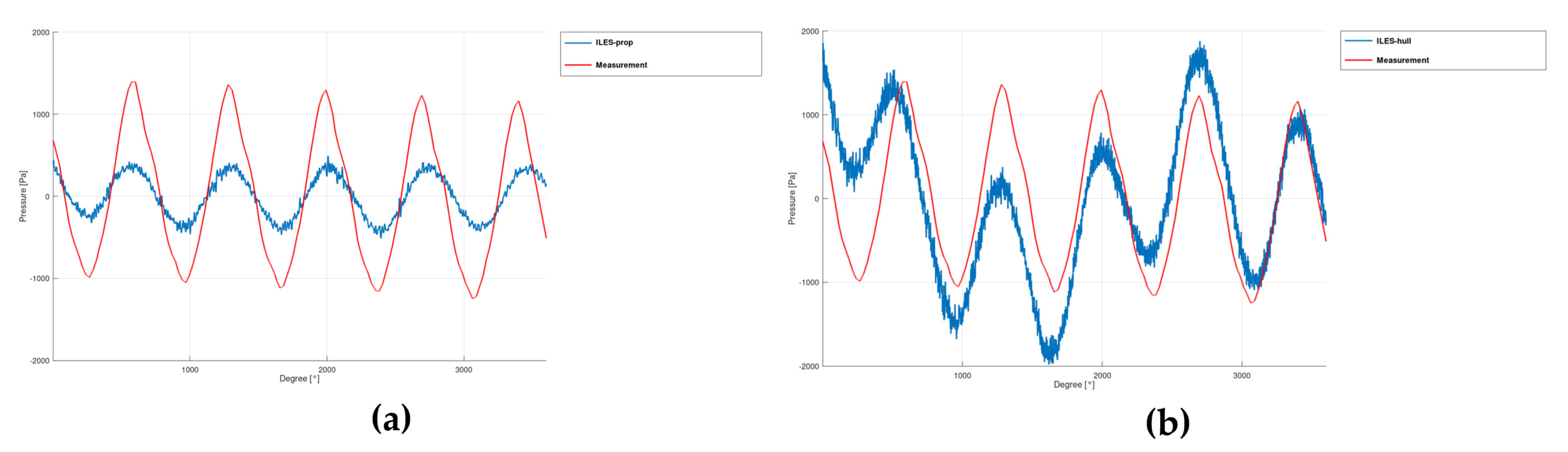
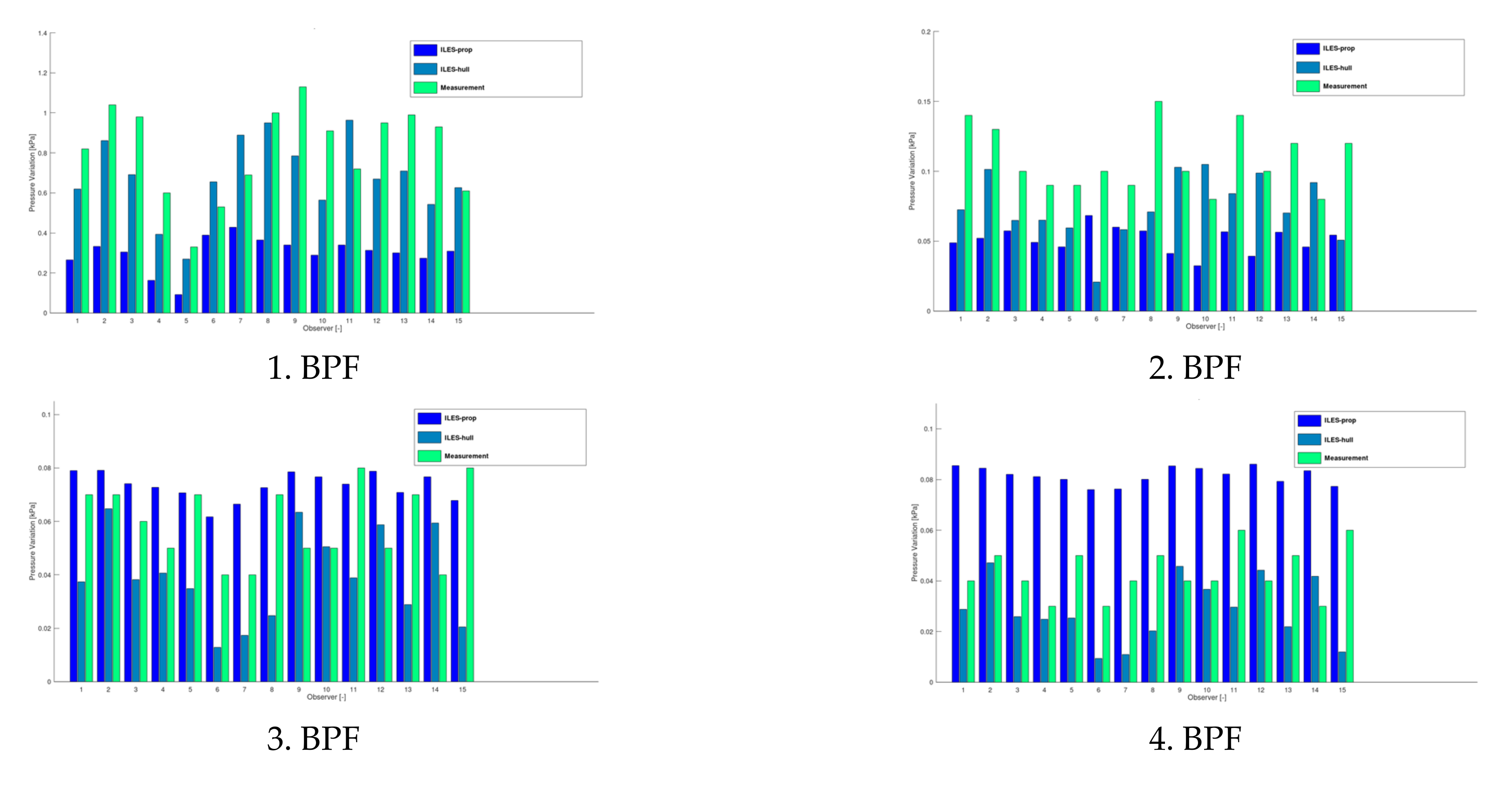
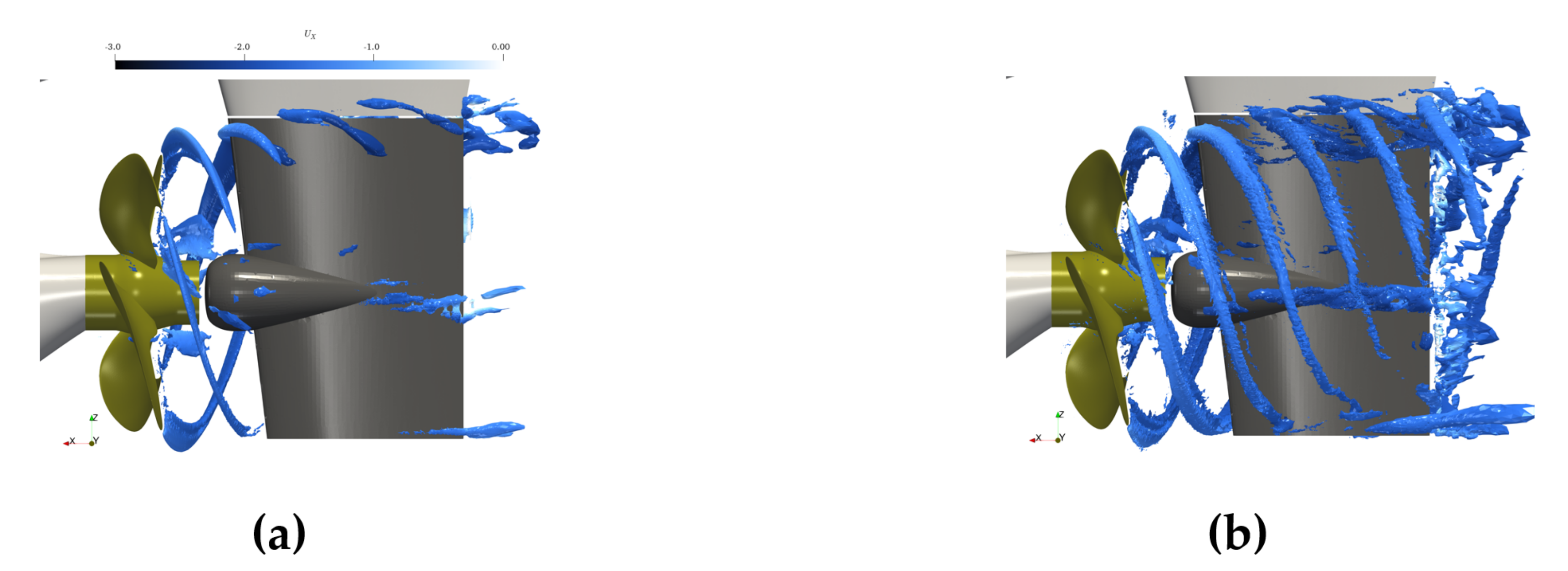
3.2. Behind Ship Investigations

3.2.1. ProNoVi Target Case

While the RANS simulation resolves the tip and hub vortex adequately, the ILES approach extends the axial reach of the same underlying mesh past the rudder, as can be seen in Figure 8. This confirms the advantages of the ILES method, by not only featuring a low cell count, but also a reduced number of transport equations compared to RANS. The rudder itself and the shaft brackets cause additional smaller eddies in their wake, which are not captured in the RANS calculation. Even without the additional adaptive mesh refinement in the tip vortex region, the propeller–rudder interaction are sufficiently resolved; however, it is expected that the mesh resolution is not adequate for capturing cavities. While the hub vortex dissolves as a result of the interaction with the rudder, the tip vortex dissipates behind the rudder, which could be an effect of the constricted flow due to the rudder or the coarser mesh.

To evaluate the capabilities of the approach employed at larger length scales, the wake fields of a twin-screw vessel obtained using the RANS and ILES approaches are further analyzed. At $x=-0.25D$ in front of the propeller plane, the difference of velocities and the standard deviation thereof is evaluated in Figure 9 in terms of Cartesian coordinates, where negative values indicate a higher velocity with RANS turbulence modeling, and the propeller radius is indicated by the outermost black circle. The velocity field is averaged over six rotations with a sampling rate of $f_s=7.4 \mathrm{kHz}$, and thus resolves wake fluctuation events over a wide range of frequencies. Overall, the velocity differences are negligible at values below 3%, with only one exception due to the wake of the propeller shaft as well as the interaction between the propeller shaft and the bearing of the A-brackets. The velocity perturbations in Figure 9b also deviate in the same region, which means that this effect could be caused by the inward rotating propeller and the accelerated flow in this region. The insufficient wall resolution of the appendages or the lack of a wall model in ILES turbulence modeling could also be causes.

In Figure 10, the observers, which are investigated in both simulation and in an experiment without cavitation, are projected onto the ship’s hull above the transparent propeller. While the experiment only considers the behind ship condition, the numerical investigation is conducted first without a hull, to quantify the difference.

Without the hull, the received pressure signals should be approximately halved compared to the measurement with the hull. An amplitude about three times greater is confirmed in the time series for the observer P10 in Figure 11, for one rotation. The blade passing frequency is the primary fluctuation in both cases, while the amplitude is very similar to the measurement in the case with the ship hull in Figure 11b. In addition to an abundance of high frequency fluctuations, a low frequency overlaying signal is detected in the second case, which could be attributed to interactions with appendages, which are intensified by the ILES modeling, or non-physical numerical pressure reflections at the cavitation tunnel walls or at domain boundaries such as inlet and outlet.

With respect to the harmonics, the effect of the hull can be better appreciated in Figure 12, as the amplitude at the first and second blade passing frequency in the free-running condition is about half of the amplitude with hull, which in turn is in very good agreement with the experiment for a large portion of the observers. For the third harmonic, the free-running results are in better agreement, as the relation between the two setups is reversed. In the case of the fourth blade frequency, the free-running setup presents a significant overprediction, while the behind hull setup presents a rather good agreement. The setups also differ as a result of the behind ship condition applying a symmetry boundary condition at the ship centerline, which leads to the acoustic results of two working propellers. This makes it even more unintuitive that the higher-order harmonics are reduced when the ship hull is included compared to the free-running propeller.

3.2.2. SCHOTTEL Reference Case 1

Similar results with respect to the axial extent of tip vortex to those in the previous case are also found for the single-screw vessel. While in the upper region of the rudder, the tip vortex structures already evolve behind the rudder in RANS, which can be attributed to the close proximity between the propeller plane and the rudder, the ILES also shows that the full tip vortex reaches behind the rudder. There are additional details of vorticity at the rudder trailing edge and the rudder bulb. On the basis of visual observation in Figure 13, the ILES approach should allow all of the important acoustic sources created by the slipstream–rudder interaction to be captured, as long as cavitation is neglected. It is curious that the tip vortex axis seems to point slightly upwards, as the vortices evolve with an angle of about 6° to the x-axis. Again, due to the rudder, an adaptive mesh refinement using the approach described in Section 2.2.1 cannot be employed to resolve the tip vortex cavitation.

In a similar investigation regarding the ship’s wake, as in the previous case, in Figure 14, obtained at $x=-0.17D$ upstream of the propeller plane, it is determined that the approach is less applicable to single-screw vessels with high block coefficients, as the propeller plane is much closer to the ship hull compared with twin-screw ships. While the in-plane components seem rather similar between RANS and ILES, at least within the propeller radius, the axial components undergo a noticeable shift immediately behind the aft bulb at the centerline, although the deviations could also indicate an issue with the interaction between the boundary layer and the outer flow. As mentioned above, a sampling frequency of $f_s=6.7 \mathrm{kHz}$ for the wake fluctuations is applied. However, the difference of the velocity perturbations over the sampling duration are less than for the twin screw case, as there are no appendages directly in the inflow of the propeller.

Figure 15 presents the cavitation results provided the simulation, which are overpredicted at the leading edge for lower radii compared to the experiment. In general, the pattern is in good agreement with the experiment; however, the inception of cavitation occurs at a slightly earlier angle. Besides the overprediction shown in the CFD results in this study, this in particular could also be caused by wake field inaccuracies arising in the ILES approach or deviations in ship geometry from the experiment, as the exact ship geometry used in the model test was not available for this simulation. The pressure observers considered in the simulation and their measurements are indicated in Figure 16 as projections onto the ship’s hull, above the propeller, the aft bulb and the rudder. In Figure 17, the cavitating case is analyzed using the KFWH method in addition to the direct pressure observations in the hydrodynamic calculation. Pressure probes and KFWH show very similar results, confirming the capabilities of the KFWH approach. Both methods lead to good agreement with the measurements directly above the propeller at the first harmonic, while the surrounding observer pressures are overpredicted. For the second harmonic, both methods overpredict the observers, while the higher harmonics overall show small deviations from the measurement. The Farassat 1A non-permeable surface formulation leads to poor agreement, which is to be expected, as the main noise sources in this case should originate from volume contributions, and sheet cavitation in particular.

3.2.3. SCHOTTEL Reference Case 2

In the case of the azimuthing twin unit in the behind ship condition, the tip vortex already extends slightly beyond the vertical shaft in the RANS calculation in Figure 18a as a result of the high cell count and the additional annulus refinements at the outer radii. Again, on the same mesh, an increase in axial extent and, more importantly, in the vortex details is achieved with ILES. Particularly noteworthy is the split of the pull propeller single tip vortex tino one main vortex and an accompanying filament after around 20% of the rotation. Behind the shaft and the push propeller hub, highly unstructured flow details are visible that do not appear in the RANS simulation. The tip vortex dissipates behind the pull propeller, although the high mesh refinement extends further, which might be a result of the interaction of the tip vortices, which purposefully lie out of phase.

The location of the pressure observers on the hull is indicated in Figure 19, with respect to the vertical shaft axis and the propellers, which are indicated together with the headbox. The pressure from the hydrodynamic calculation is recorded, and the amplitudes at the first and second blade passing frequencies are scaled to full scale, in order to compare them with the scaled experimental measurements in Figure 20. Acceptable agreement is achieved for most observers at the first harmonic, with the prediction generally underestimating the experiment slightly. Inversely, the second harmonic results overall are higher than the experimental observations. On the basis of the results of the simulation and the experiment, an improved propeller design is created with the aim of lowering the maximum pressure pulses to values below $\mathsf{\Delta }{p}^{\prime }<0.8 \mathrm{kPa}$, proving that it is possible to detect the effects of minor design changes in the predicted acoustic emissions.

4. Discussion

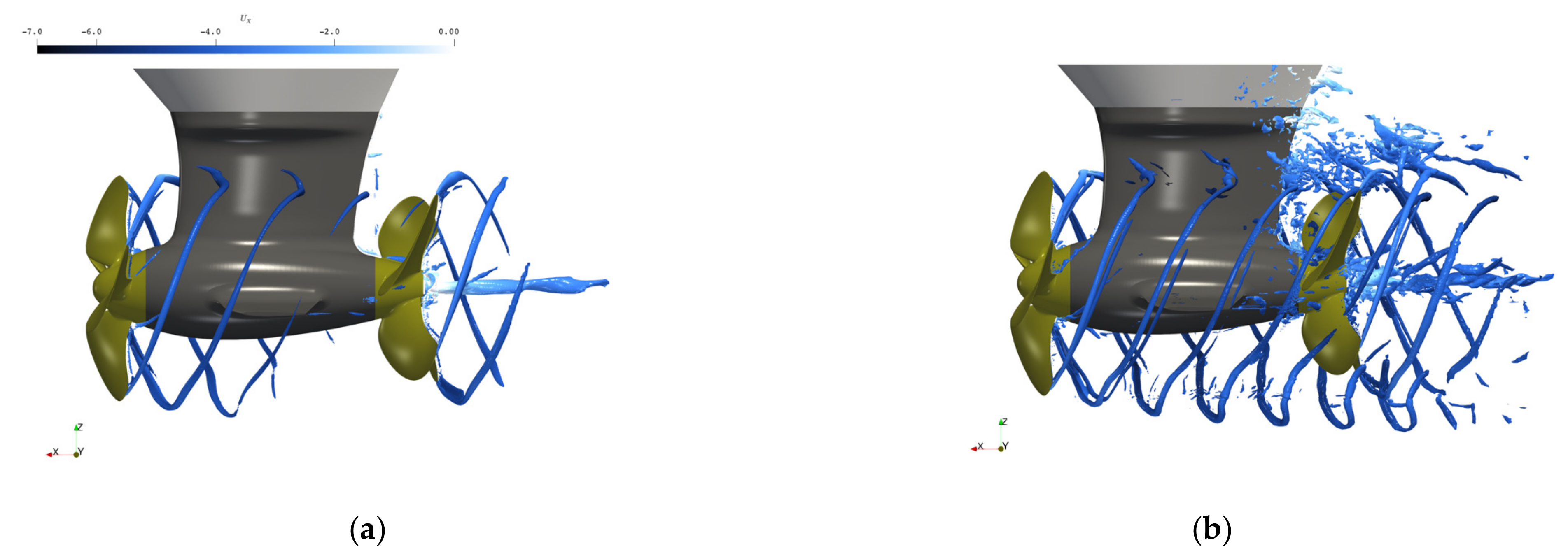
4.1. Noise Generation Mechanisms

The presented evaluation of the acoustic pressure level shows that acceptable agreement with the experiments was achieved for the Newcastle test case with respect to the full-scale corrected sound level. The distinct modeling steps:

• Resolved turbulence,
• Phase transition model, and
• Vorticity-based refinements,

Each of which add further details to the physical description of the flow field, reducing the difference between prediction and measurement. However, the lower sound levels in the medium frequencies between 0.1 and 3 kHz as a result of activating cavitation is unexpected. Although similar tendencies have been reported from measurements before [29]. The decrease of the sound levels by activating cavitation in the simulation could be facilitated by the following mechanisms:

• Reduction of pressure wave propagation by the vapor phase, which dampens the noise, as has been reported in some experiments with steady cavitation;
• Overall, only moderate variation of cavitation volume as a result of the steady tip vortex cavity, which adds purely sinusoidal disturbance to the flow, but no broadband noise.

As mentioned in the Introduction, other authors have detected an increase of the sound level in this frequency range as an effect of single bubble inclusion. Thus, it is questionable whether the VOF method is adequate for resolving the significant broadband contributions of propeller-induced cavitation to underwater radiated noise, which in turn is highly dependent on the propeller geometry. Another explanation could be the lack of an unsteady excitation of the tip vortex cavity, which in reality is applied constantly by the turbulent unsteady inflow.

Although the Newcastle test case is recommended by the ITTC for acoustic investigations, the round robin test setup from the selected reference results in a complex CFD setup, due to the cross section of the small tunnel and modeling assumptions with respect to the inlet and outlet, which generates additional uncertainty that cannot be described quantitatively by the numerical methods at their current stage. Thus, an innovative test case in a quasi-infinite domain, by employing effective mitigation of pressure reflections could lead to an improved understanding of methods for underwater radiated noise simulation.

4.2. Practical Application in the Near Field

The hydrodynamic calculation with ILES in combination with the Schnerr-Sauer cavitation model proves to be a computationally cheap and high-quality modeling technique for free-running propellers and propellers in the behind ship condition that captures the turbulence and cavitation details, which are expected to be the main mechanisms behind propeller noise generation. With advanced mesh refinement methods, the intricate trailing vortex cavitation structures in the propeller slipstream can be resolved; however, the simple approach presented in part 1 and used in Section 3.1 is not feasible with non-axisymmetric ship or propulsion unit structures downstream of the propeller or highly oblique flow conditions. To overcome the first issue, overset grid functionalities could be employed, which rotate a static refinement through solid structures such as rudders. Another technique would be to apply automatic adaptive mesh refinement methods involving a dynamic refinement and coarsening of the cells occurring depending on a flow criterion; however, it is questionable whether this could be implemented with an acceptable numerical effort.

Free-running propeller noise signatures can be predicted in the near field with CFD domain pressure within the margins of reproducibility of the model-scale measurements. In the case of a sufficiently refined mesh, the pressure signals observed within the hydrodynamic solution, which can be employed to determine the incompressible pressure fluctuations on the hull, are a good approximation of the experimental values at model and full scale. For far field noise analysis, decoupled acoustic propagation methods such as the FWH method are essential, as the observers may be located outside the CFD domain, and acoustic effects, such as the speed of sound or reflections, which are not considered, become important. The permeable surface formulation yields good results, as it can take into account volume contributions; however, the sensitivity on extent and position of the control surface leads to more questions than answers, requiring additional studies. Overall, the excellent agreement with the hydrodynamic solution in combination with the good agreement with the measurements validates the acoustic method for its intended purpose in the near field and suggests that the main deviations to measurements arise in the hydrodynamic part of the simulation, which makes the proposed approach feasible and appropriate for far-field calculations.

5. Conclusions

The approach for determining the far field URN of a propeller in behind-ship condition with ILES without a wall model in combination with the permeable surface FWH method is suggested as a computationally less expensive alternative to the traditional LES and DES methods. A higher level of detail with respect to the cavity structure in the tip vortex region, which is expected to influence acoustic emissions, is employed by employing a single Q-criterion-based a priori mesh refinement step, which is required only to refine the cavitating diameter, in order to keep the mesh size low. By comparing the acoustic spectra of the cavitation tunnel model test, the accuracy of this approach with respect to the prediction of URN in the near field was estimated to be good within the margins of reproducibility of the measurements.

This approach is only possible when the inflow at the propeller is straight and no structural obstacles are interacting with the propeller slipstream, which is typically not the case for propeller–hull combinations with rudders or azimuthing propulsors. In the test cases in the behind ship condition, the tip vortex refinement step could not be executed; however, adequate results were still produced without mesh refinement when comparing their acoustic emissions to measurements in the near field with incompressible hull pressure fluctuations. For these near field observers, the permeable surface FWH method produces results that are of similar quality to the pressure obtained from the hydrodynamic solution, and presented accuracy that was adequate for the propeller design process and qualification of vessel propeller combinations.

In summary, the method described here produces good predictions of near-field acoustic pressure, and could be a feasible way of estimating URN in the far field by considering resolved turbulence and cavitation for propeller–hull configurations in industrial environments. However, the trailing vortex cavity refinements in the slipstream of the propeller have to be adjusted to allow for more complex geometries. In addition, validation with measurements in the far field is necessary, which is quite complex due to the inherent nature of the experimental conditions at full scale, including weather and reflections as a result of underwater terrain or the free water surface.

References

1. Frisk, G.V. Noiseonomics: The relationship between ambient noise levels in the sea and global economic trends. Sci. Rep. 2012, 2, 437. [Google Scholar] [CrossRef] [PubMed] [Green Version]
2. Wisniewska, D.M.; Johnson, M.; Teilmann, J.; Siebert, U.; Galatius, A.; Dietz, R.; Madsen, P.T. High rates of vessel noise disrupt foraging in wild harbour porpoises (Phocoena phocoena). Proc. R. Soc. B 2018, 285, 20172314. [Google Scholar] [CrossRef] [PubMed] [Green Version]
3. Wysocki, L.E.; Dittami, J.P.; Ladich, F. Ship noise and cortisol secretion in European freshwater fishes. Biol. Conserv. 2005, 128, 501–508. [Google Scholar] [CrossRef]
4. DNV GL. Rules for the Classification Ship, Part 6 Additional Class Notation Chapter 7 Environmental Protection and Pollutrion Control. 2017. Available online: https://rules.dnv.com/docs/pdf/DNV/ru-ship/2017-01/DNVGL-RU-SHIP-Pt6Ch7.pdf (accessed on 16 July 2021).
5. Bretschneider, H.; Bosschers, J.; Choi, G.H.; Ciappi, E.; Farabee, T.; Kawakita, C.; Tang, D. Specialist Committee on Hydrodynamic Noise; ITTC: Copenhagen, Denmark, 2014. [Google Scholar]
6. IMO. Guidelines for the Reduction of Underwater Noise from Commercial Shipping to Address Adverse Impacts on Marine Life; IMO: London, UK, 2014. [Google Scholar]
7. Wittekind, D.; Schuster, M. Propeller cavitation noise and background noise in the sea. Ocean Eng. 2016, 120, 116–121. [Google Scholar] [CrossRef]
8. Van Wijngaarden, E. Prediction of Propeller-Induced Hull-Pressure Fluctuations; Maritime Research Institute Netherlands: Wageningen, The Netherlands, 2011. [Google Scholar]
9. Kim, S.; Kinnas, S.A. Prediction of unsteady developed tip vortex cavitation and its effect on the induced hull pressures. In Proceedings of the Sixth International Symposium on Marine Propulsors, Rome, Italy, 26–30 May 2019. [Google Scholar]
10. Göttsche, U.; Lampe, T.; Scharf, M.; Abdel-Maksoud, M. Evaluation of underwater sound propagation of a catamaran with cavitating propellers. In Proceedings of the Sixth International Symposium on Marine Propulsors, Rome, Italy, 26–30 May 2019. [Google Scholar]
11. Bensow, R.E.; Liefvendahl, M. Implicit and explicit subgrid modeling in les applied to a marine propeller. In Proceedings of the 38th Fluid Dynamics Conference and Exhibit, Seattle, WA, USA, 23–26 June 2008. [Google Scholar]
12. Kimmerl, J.; Mertes, P.; Abdel-Maksoud, M. Application of large eddy simulation to predict underwater noise of marine propulsors. Part 1 Cavitation Dynamics. Ocean Eng. 2021. In Press. [Google Scholar]
13. Bensow, R.E.; Liefvendahl, M. An acoustic analogy and scale-resolving flow simulation methodology for the prediction of propeller radiated noise. In Proceedings of the 31st Symposium on Naval Hydrodynamics, Monterey, CA, USA, 11–16 September 2016. [Google Scholar]
14. Kinnas, S.; Abdel-Maksoud, M.; Barkmann, U.; Lübke, L.; Tian, Y. Proceedings of the Second Workshop on Cavitation and Propeller Performance. In Proceedings of the The Fourth International Symposium on Marine Propulsors, Austin, TX, USA, 31 May–4 June 2015. [Google Scholar]
15. Yilmaz, N.; Atlar, M.; Fitzsimmons, P. An improved tip vortex cavitation model for propeller-rudder interaction. In Proceedings of the 10th International Cavitation Symposium, Baltimore, MD, USA, 14–16 May 2018. [Google Scholar]
16. Yilmaz, N.; Aktas, B.; Atlar, M.; Fitzsimmons, P.; Felli, M. An experimental and numerical investigation of propeller-rudder-hull interaction in the presence of tip vortex cavitation (TVC). Ocean Eng. 2020, 216, 108024. [Google Scholar] [CrossRef]
17. Lidtke, K. Predicting Radiated Noise of Marine Propellers Using Acoustic Analogies and Hybrid Eulerian-Lagrangian Cavitation Models. Ph.D. Thesis, University of Southampton, Southampton, UK, 2017. [Google Scholar]
18. Liefvendahl, M.; Bensow, R. Simulation-based analysis of flow-generated noise from cylinders with different cross-sections. In Proceedings of the 32nd Symposium on Naval Hydrodynamics, Hamburg, Germany, 5–10 August 2018. [Google Scholar]
19. Sezen, S.; Atlar, M.; Fitzsimmons, P. Prediction of cavitating propeller underwater radiated noise using RANS & DES-based hybrid method. In Ships and Offshore Structures; Taylor & Francis: Abingdon, UK, 2021. [Google Scholar]
20. Kimmerl, J.; Mertes, P.; Abdel-Maksoud, M. Application of large eddy simulation to predict underwater noise of marine propulsors. part 1 cavitation dynamics. J. Mar. Sci. Eng. 2021, 6, 56. [Google Scholar]
21. Kimmerl, J.; Mertes, P.; Abdel-Maksoud, M. Turbulence modelling capabilities of iles for propeller induced urn prediction. In Proceedings of the SNAME Maritime Convention 2020, Houston, TX, USA, 29 September–1 October 2020. [Google Scholar]
22. Tani, G.; Viviani, M.; Felli, M.; Lafeber, F.H.; Lloyd, T.; Aktas, B.; Atlar, M.; Seol, H.; Hallander, J.; Sakamoto, N.; et al. Round robin test on radiated noise of a cavitating propeller. In Proceedings of the Sixth International Symposium on Marine Propulsors, Rome, Italy, 26–30 May 2019. [Google Scholar]
23. Williams, J.E.F.; Hawkings, D.L. Sound generation by turbulence and surfaces in arbitrary motion. Philos. Trans. R. Soc. Lond. Ser. Math. Phys. Sci. 1969, 264, 321–342. [Google Scholar]
24. Lidtke, K.; Lloyd, T.; Vaz, G. Acoustic modelling of a propeller subject to non-uniform inflow. In Proceedings of the Sixth International Symposium on Marine Propulsors, Rome, Italy, 26–30 May 2019. [Google Scholar]
25. Sagaut, P. Large Eddy Simulation for Incompressible Flows; Springer: New York, NY, USA, 2006. [Google Scholar]
26. Kuiper, G. Cavitation Inception on Ship Propeller Models. Ph.D. Thesis, TU Delft, Wageningen, The Netherlands, 1981. [Google Scholar]
27. Tani, G.; Aktas, B.; Viviani, M.; Atlar, M. Two medium size cavitation tunnel hydro-acoustic benchmark experiment comparisons as part of a round robin test campaign. Ocean Eng. 2017, 138, 179–207. [Google Scholar] [CrossRef] [Green Version]
28. Bosschers, J. Analysis of inertial waves on inviscid cavitating vortices in relation to lowfrequency radiated noise. In Proceedings of the Warwick Innovative Manufacturing Research Centre (WIMRC) Cavitation: Turbo-Machinery and Medical Applications Forum, Warwick, UK, 24 March 2008. [Google Scholar]
29. Pennings, P.; Westerweel, J.; van Terwisga, T. Cavitation tunnel analysis of radiated sound from the resonance of a propeller tip vortex cavity. Int. J. Multiph. Flow 2016, 83, 1–11. [Google Scholar] [CrossRef] [Green Version]
Figure 1. Initial mesh: (a) Newcastle; (b) P1595.
Jmse 09 00778 g001
Figure 2. Newcastle. Distance refinement in tip vortex region based on Q -criterion Q = 5 10 5   s 2 for condition C2.
Jmse 09 00778 g002
Figure 3. Behind ship mesh: (a) ProNoVi Target Case; (b) SCHOTTEL Reference Case 1; (c) SCHOTTEL Reference Case 2.
Jmse 09 00778 g003
Figure 4. Newcastle. Acoustic investigation: (a) numerical setup with pressure observers H1-H3; (b) comparison of the SL for different solvers with the averaged measurement, condition C1, observer H2.
Jmse 09 00778 g004
Figure 5. Newcastle. SL for the three pressure observers with measurement for the conditions: (a) C1; (b) C2; (c) C3; (d) C6.
Jmse 09 00778 g005
Figure 6. P1595. Acoustic investigation: (a) numerical setup with pressure observer; (b) cavitation isosurface.
Jmse 09 00778 g006
Figure 7. P1595. Sound pressure level spectral evaluation at observer: comparison of KFWH approach under cavitating and non-cavitating conditions with experimental measurements from SINTEF Ocean.
Jmse 09 00778 g007
Figure 8. ProNoVi target case. Comparison of RANS and ILES Q-criterion Q = 5 10 4   s 2 at model scale on the same mesh: (a) RANS; (b) ILES.
Jmse 09 00778 g008
Figure 9. ProNoVi target case. Difference between RANS and ILES wake field in the Cartesian components x, y and z, velocities averaged over time, propeller plane indicated by radii sections: (a) velocity difference; (b) velocity standard deviation difference.
Jmse 09 00778 g009
Figure 10. ProNoVi target case. Locations of the acoustic observers on the hull with respect to the propeller and the headbox of the unit in full scale.
Jmse 09 00778 g010
Figure 11. ProNoVi target case. Comparison of ILES time signal excerpts: (a) propeller only; (b) propeller and hull.
Jmse 09 00778 g011
Figure 12. ProNoVi Target Case. Pressure amplitudes at multiples of the blade passing frequency (BPF) in comparison to the experiment with the model propeller only and the model propeller and ship hull in the propulsion condition with the results scaled to full scale.
Jmse 09 00778 g012
Figure 13. SCHOTTEL reference case 1. Comparison of RANS and ILES Q-criterion Q = 5 10 2   s 2 at model scale on the same mesh: (a) RANS; (b) ILES.
Jmse 09 00778 g013
Figure 14. SCHOTTEL reference case 1. Differences between the RANS and ILES wake fields in terms of Cartesian components x, y and z, velocities are averaged over one rotation, the propeller plane is indicated by radii sections: (a) velocity difference; (b) velocity standard deviation difference.
Jmse 09 00778 g014
Figure 15. SCHOTTEL reference case 1. The cavitation region (white) and pressure coefficient with one propeller blade located at 12 o’clock position.
Jmse 09 00778 g015
Figure 16. SCHOTTEL reference case 1. Locations of the acoustic observers on the hull with respect to the propeller and the rudder of the unit at full scale; observers are symmetrical to the centerline.
Jmse 09 00778 g016
Figure 17. SCHOTTEL reference case 1. Pressure amplitudes obtained with the direct pressure and KFWH method at blade passing frequencies (BPF) in comparison to the experiment at full scale in propulsion condition with cavitation.
Jmse 09 00778 g017
Figure 18. SCHOTTEL reference case 2. Comparison of RANS and ILES Q-criterion Q = 1 10 4 s 2 at model scale on the same mesh: (a) RANS; (b) ILES.
Jmse 09 00778 g018
Figure 19. SCHOTTEL reference case 2. Locations of acoustic observers on the hull with respect to the origin located at the vertical shaftline with propellers and the headbox of the unit at model scale; observers are symmetrical to the centerline.
Jmse 09 00778 g019
Figure 20. SCHOTTEL reference case 2. Pressure amplitudes at multiples of the blade passing frequency (BPF) in comparison to the experiment and a revised propeller design with model propeller and ship hull and the results scaled to full scale.
Jmse 09 00778 g020