
Long-Term Trends of Sea Surface Wind in the Northern South China Sea under the Background of Climate Change

Abstract
:1. Introduction
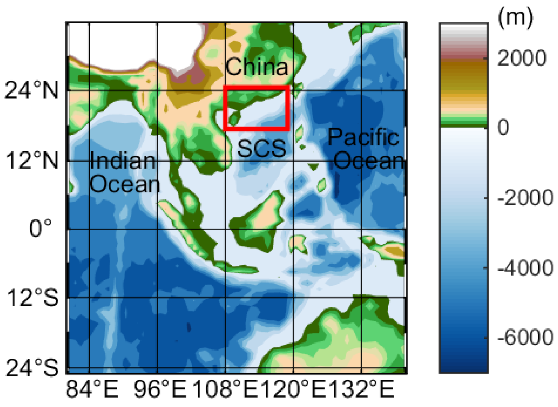
2. Study Area
3. Data and Methodology
3.1. Data
3.2. Methodology
3.2.1. Mann–Kendall Test
3.2.2. Cross-Wavelet Transform
4. Results and Discussion
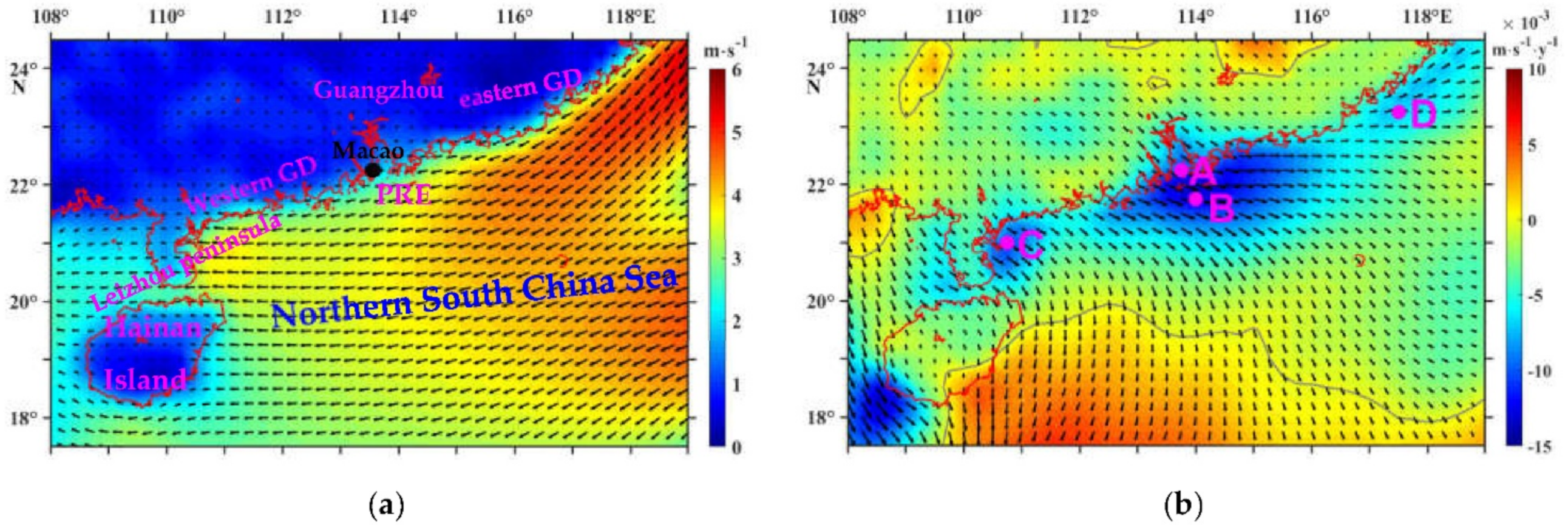
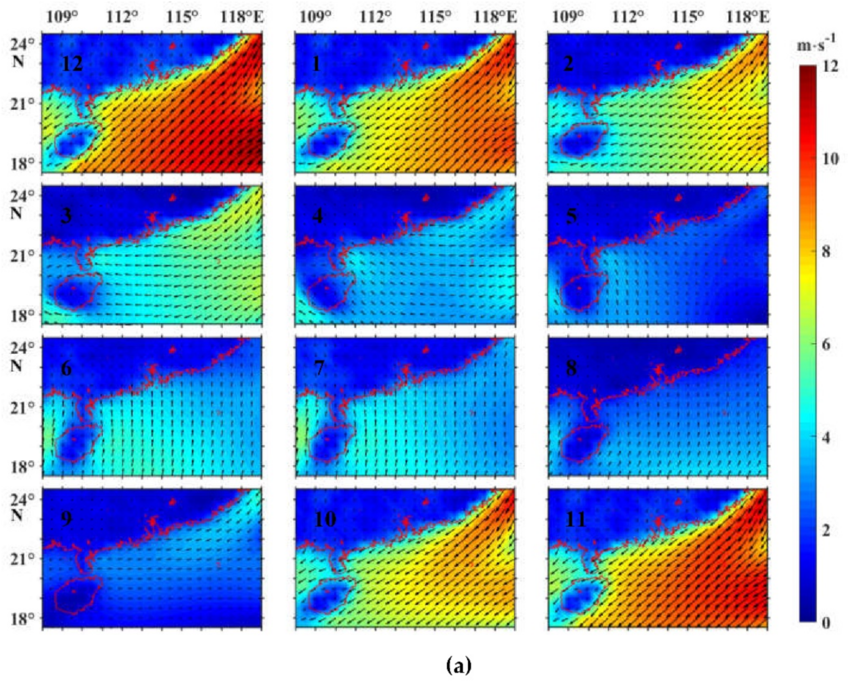
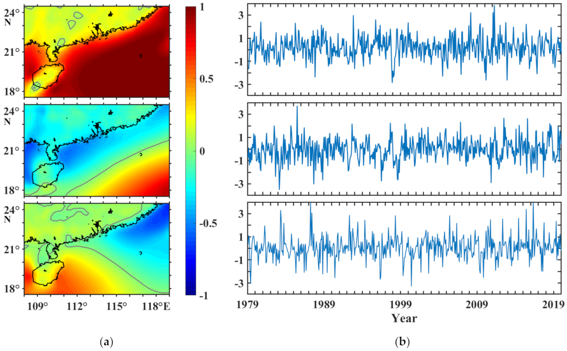
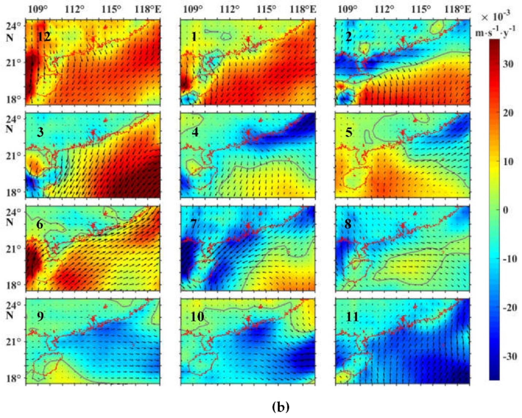
4.1. Spatial Variation of the Wind Field in the Northern SCS
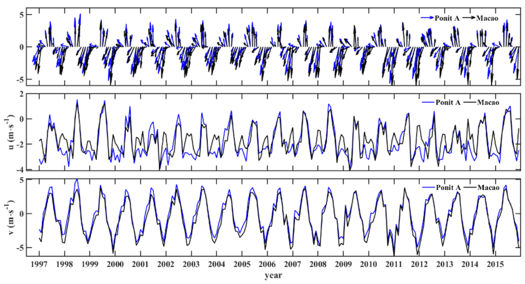
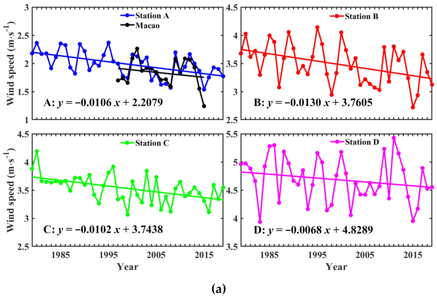
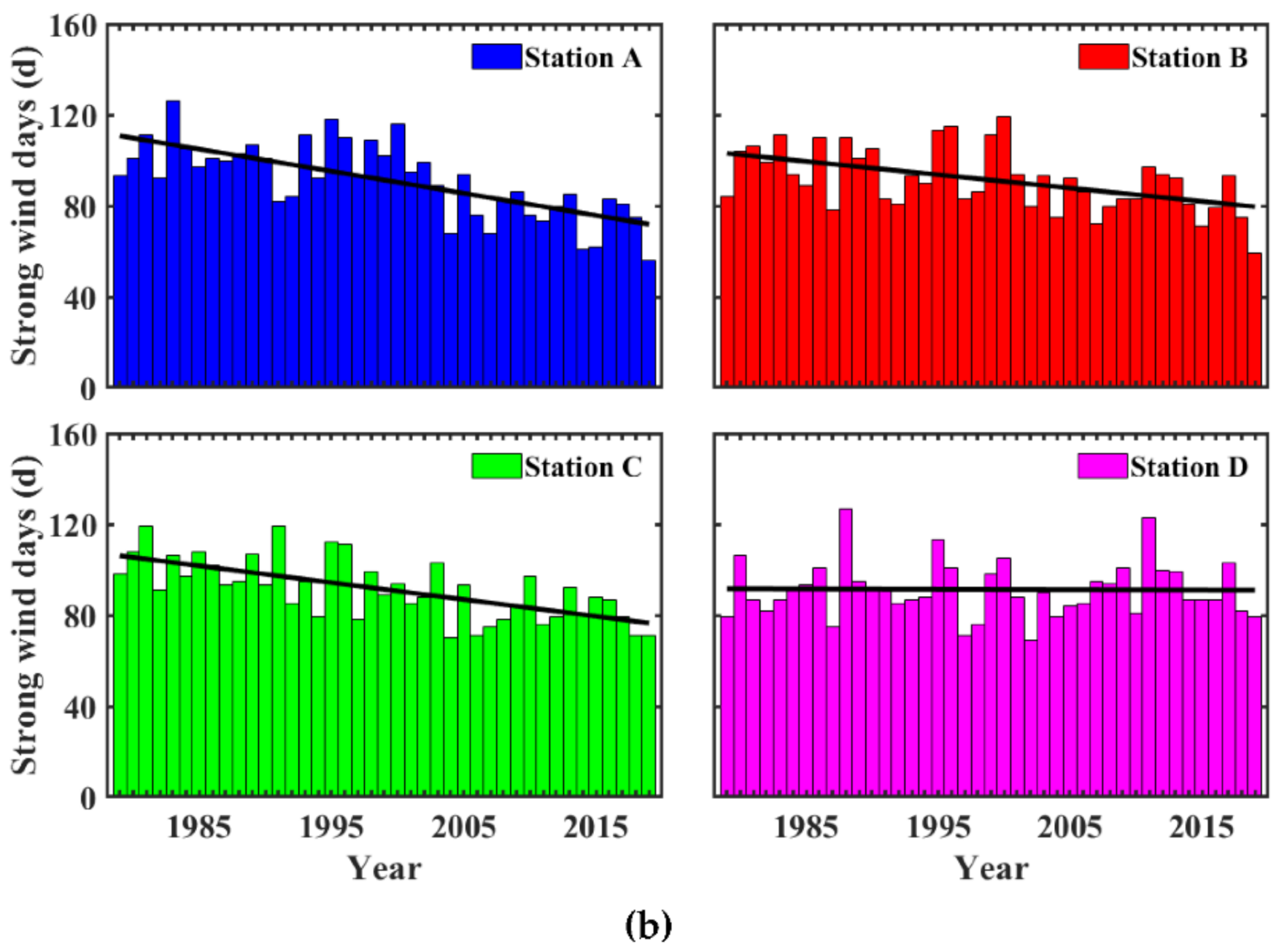
4.2. Wind Field Trends in Typical Areas
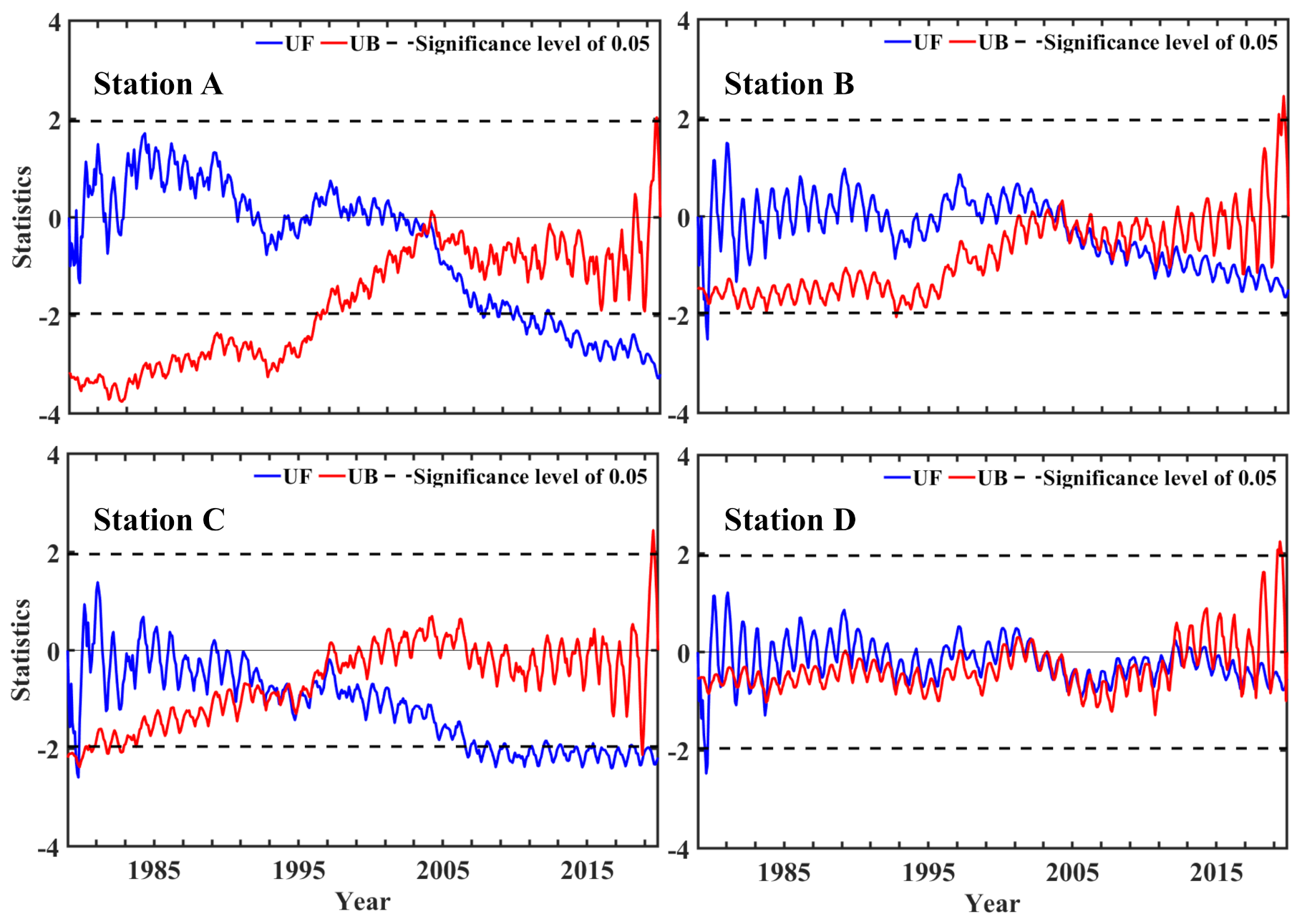
4.3. M–K Test of the Wind Fields in Representative Areas
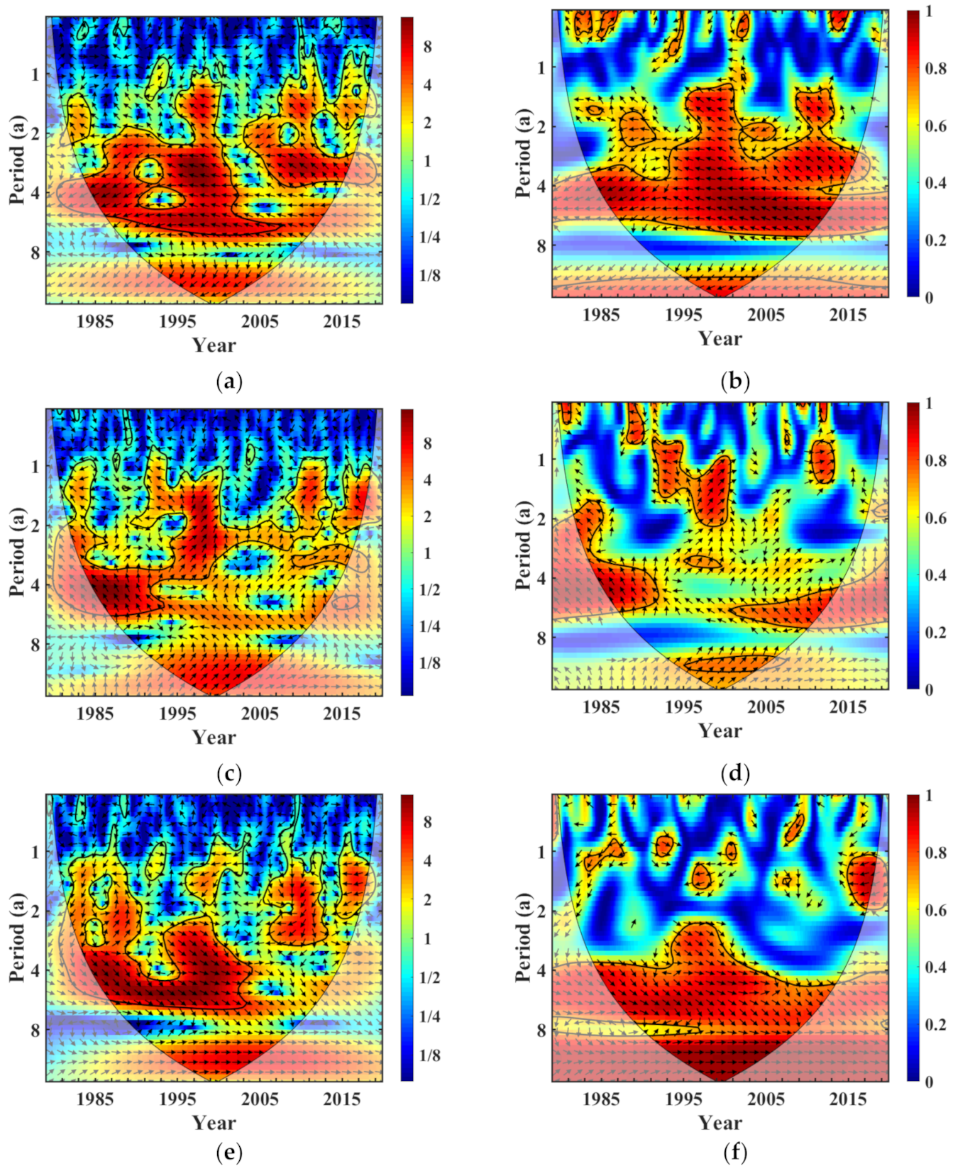
4.4. Correlation between the Interannual Variation of the Wind Field and ENSO
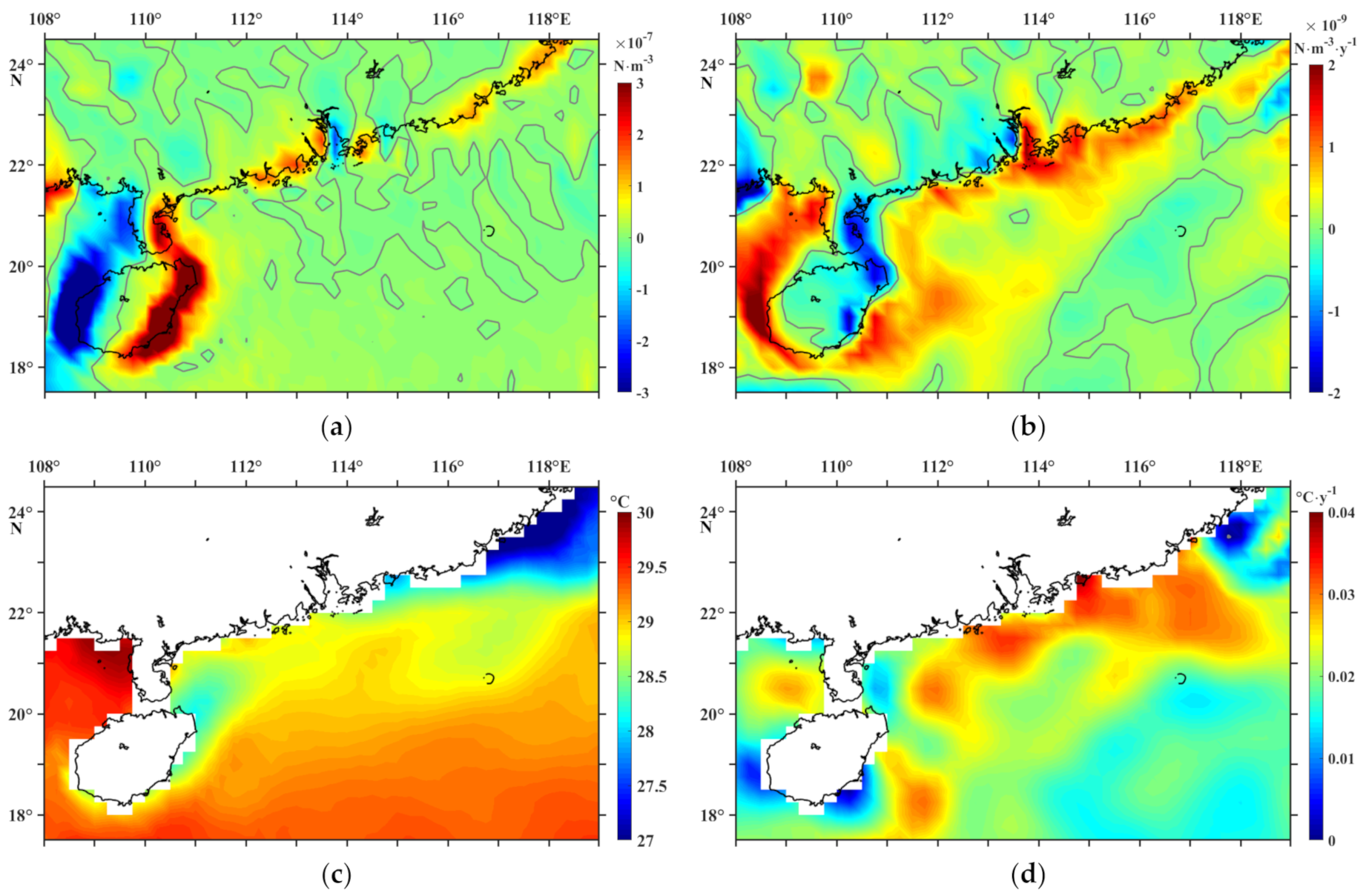
4.5. Long-Term Trends of Wind Stress Curl and Effects on Coastal Upwelling
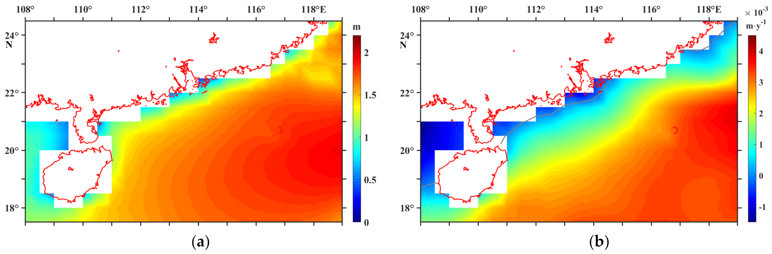
4.6. Effect of the Trend of Wind Stress on Significant Wave Height
5. Conclusions
Author Contributions
Funding
Institutional Review Board Statement
Informed Consent Statement
Data Availability Statement
Acknowledgments
Conflicts of Interest
References
- Wang, B.; Huang, F.; Wu, Z.; Yang, J.; Fu, X.; Kikuchi, K. Multi-scale climate variability of the South China Sea monsoon: A review. Dyn. Atmos. Oceans 2009, 47, 15–37. [Google Scholar] [CrossRef]
- Cui, K.; Sun, J.; Xue, F. Analysis of the spatial and temporal characteristics of sea surface wind field in the North Indian Ocean. Trans. Oceanol. Limnol. 2013, 4, 34–42. Available online: http://en.cnki.com.cn/Article_en/CJFDTOTAL-HYFB201304005.htm (accessed on 20 March 2021).
- Parvathi, V.; Suresh, I.; Lengaigne, M.; Izumo, T.; Vialard, J. Robust Projected Weakening of Winter Monsoon Winds Over the Arabian Sea Under Climate Change. Geophys. Res. Lett. 2017, 44, 9833–9843. [Google Scholar] [CrossRef]
- Dong, S.; Gong, Y.; Wang, Z. Long-term variations of wind and wave conditions in the Taiwan Strait. Reg. Stud. Mar. Sci. 2020, 36, 101256. [Google Scholar] [CrossRef]
- Gai, C.; Liu, Q.; Roberts, A.P.; Chou, Y.; Zhao, X.; Jiang, Z.; Liu, J. East Asian monsoon evolution since the late Miocene from the South China Sea. Earth Planet. Sci. Lett. 2020, 530, 115960. [Google Scholar] [CrossRef]
- Islek, F.; Yuksel, Y.; Sahin, C. Spatiotemporal long-term trends of extreme wind characteristics over the Black Sea. Dyn. Atmos. Oceans 2020, 90, 101132. [Google Scholar] [CrossRef]
- Yang, C.; Dang, H.; Zhou, X.; Zhang, H.; Wang, X.; Wang, Y.; Qiao, P.; Jiang, X.; Jian, Z. Upper ocean hydrographic changes in response to the evolution of the East Asian monsoon in the northern South China Sea during the middle to late Miocene. Glob. Planet. Chang. 2021, 201, 103478. [Google Scholar] [CrossRef]
- Tamburini, F.; Adatte, T.; Föllmi, K.; Bernasconi, S.; Steinmann, P. Investigating the history of East Asian monsoon and climate during the last glacial–interglacial period (0–140,000 years): Mineralogy and geochemistry of ODP Sites 1143 and 1144, South China Sea. Mar. Geol. 2003, 201, 147–168. [Google Scholar] [CrossRef]
- Shi, N. Features of the East Asian winter monsoon intensity on multiple time scale in recent 40 years and their relation to climate. J. Appl. Meteor. Sci. 1996, 7, 175–182. Available online: http://en.cnki.com.cn/Article_en/CJFDTOTAL-YYQX602.006.htm (accessed on 20 March 2021).
- Yang, M.; Xu, H.; Li, W.; Liu, Y. Variations of East Asian monsoon and its relationships with land-sea temperature in recent 40 years. J. Appl. Meteor. Sci. 2008, 19, 522–530. [Google Scholar] [CrossRef]
- Jiang, Y.; Luo, Y.; Zhao, Z.; Tao, S. Changes in wind speed over China during 1956–2004. Theor. Appl. Clim. 2009, 99, 421–430. [Google Scholar] [CrossRef]
- Jiang, Y.; Luo, Y.; Zhao, Z. Maximum wind speed changes over China. Acta Meteorol. Sin. 2013, 27, 63–74. [Google Scholar] [CrossRef]
- Shi, P.-J.; Zhang, G.-F.; Kong, F.; Ye, Q. Wind speed change regionalization in China (1961–2012). Adv. Clim. Chang. Res. 2015, 6, 151–158. [Google Scholar] [CrossRef]
- Mo, H.; Hong, H.; Fan, F. Estimating the extreme wind speed for regions in China using surface wind observations and reanalysis data. J. Wind. Eng. Ind. Aerodyn. 2015, 143, 19–33. [Google Scholar] [CrossRef]
- Dai, N.; Xie, A.; Zhang, Y. Interannual and interdecadal variations of summer monsoon activities over South China Sea. Clim. Environ. Res. 2000, 5, 363–374. [Google Scholar] [CrossRef]
- Zhang, X.; Li, J.; Ding, Y.; Yan, J. A study of circulation characteristics and index of South China Sea summer monsoon. Acta Meteorol. Sin. 2001, 15, 450–464. [Google Scholar] [CrossRef]
- Liang, J.; Yang, S.; Li, C.; Li, X. Long-term changes in the South China Sea summer monsoon revealed by station observations of the Xisha Inland. J. Geophys. Res-Atmos. 2007, 112, D10104. [Google Scholar] [CrossRef]
- Ward, M.N.; Hoskins, B.J. Near-surface wind over the Global Ocean 1949–1988. J. Climate 1996, 9, 1877–1895. [Google Scholar] [CrossRef] [Green Version]
- Gulev, S.K.; Grigorieva, V. Last century changes in ocean wind wave height from global visual wave data. Geophys. Res. Lett. 2004, 31, 24302. [Google Scholar] [CrossRef]
- Gulev, S.K.; Hasse, L. Changes of wind waves in the North Atlantic over the last 30 years. Int. J. Climatol. 1999, 19, 1091–1117. [Google Scholar] [CrossRef]
- Gower, J.F.R. Temperature, Wind and Wave Climatologies, and Trends from Marine Meteorological Buoys in the Northeast Pacific. J. Clim. 2002, 15, 3709–3718. [Google Scholar] [CrossRef]
- Young, I.R.; Zieger, S.; Babanin, A. Global Trends in Wind Speed and Wave Height. Science 2011, 332, 451–455. [Google Scholar] [CrossRef] [PubMed]
- Wilson, R.E.; Swanson, R.L.; Crowley, H.A. Perspectives on long-term variations in hypoxic conditions in western Long Island Sound. J. Geophys. Res. Space Phys. 2008, 113, 12011. [Google Scholar] [CrossRef] [Green Version]
- Scully, M. The importance of decadal-scale climate variability to wind-driven modulation of hypoxia in Chesapeake Bay. Nat. Précéd. 2009, 40, 1345–1400. [Google Scholar] [CrossRef]
- Hong, B.; Wang, G.; Xu, H.; Wang, D. Study on the Transport of Terrestrial Dissolved Substances in the Pearl River Estuary Using Passive Tracers. Water 2020, 12, 1235. [Google Scholar] [CrossRef]
- Yu, L.; Gan, J.; Dai, M.; Hui, C.R.; Lu, Z.; Li, D. Modeling the role of riverine organic matter in hypoxia formation within the coastal transition zone off the Pearl River Estuary. Limnol. Oceanogr. 2021, 66, 452–468. [Google Scholar] [CrossRef]
- Zhao, H.; Dai, M.; Gan, J.; Zhao, X.; Lu, Z.; Liang, L.; Liu, Z.; Su, J.; Cao, Z. River-dominated pCO2 dynamics in the northern South China Sea during summer: A modeling study. Prog. Oceanogr. 2021, 190, 102457. [Google Scholar] [CrossRef]
- Zhu, L.; Zhang, H.; Guo, L.; Huang, W.; Gong, W. Estimation of riverine sediment fate and transport timescales in a wide estuary with multiple sources. J. Mar. Syst. 2020, 214, 103488. [Google Scholar] [CrossRef]
- Pan, J.; Gu, Y.; Wang, D. Observations and numerical modeling of the Pearl River plume in summer season. J. Geophys. Res. Oceans 2014, 119, 2480–2500. [Google Scholar] [CrossRef]
- Jing, Z.; Qi, Y.; Du, Y. Upwelling in the continental shelf of northern South China Sea associated with 1997-1998 El Niňo. J. Geophys. Res-Oceans. 2011, 116, C02033. [Google Scholar] [CrossRef]
- Lin, P.; Gan, J.; Hu, J. Coastal Upwelling in the Northern South China Sea. Reg. Oceanogr. South China Sea 2020, 11, 289–322. [Google Scholar] [CrossRef]
- Shu, Y.; Wang, D.; Feng, M.; Geng, B.; Chen, J.; Yao, J.; Xie, Q.; Liu, Q.-Y. The Contribution of Local Wind and Ocean Circulation to the Interannual Variability in Coastal Upwelling Intensity in the Northern South China Sea. J. Geophys. Res. Oceans 2018, 123, 6766–6778. [Google Scholar] [CrossRef]
- Wu, R.; Li, L. Summarization of study on upwelling system in the South China Sea. J. Oceanogr. Taiwan Strait 2003, 22, 269–276. [Google Scholar] [CrossRef]
- Zhuang, W.; Wang, D.X.; Hu, J.Y.; Ni, W.S. Response of the cold water mass in the western South China Sea to the wind stress curl associated with summer monsoon. Acta Meteorol. Sin. 2006, 25, 1–13. [Google Scholar] [CrossRef]
- Hersbach, H.; Bell, B.; Berrisford, P.; Hirahara, S.; Horanyi, A.; Muñoz-Sabater, J.; Nicolas, J.; Peubey, C.; Radu, R.; Schepers, D.; et al. The ERA5 global reanalysis. Q. J. R. Meteorol. Soc. 2020, 146, 1999–2049. [Google Scholar] [CrossRef]
- Bonavita, M.; Hólm, E.; Isaksen, L.; Fisher, M. The evolution of the ECMWF hybrid data assimilation system. Q. J. R. Meteorol. Soc. 2016, 142, 287–303. [Google Scholar] [CrossRef]
- Kendall, M.G. Rank Correlation Methods, 4th ed.; Charles Griffin: London, UK, 1975; p. 202. [Google Scholar]
- Haktanir, T.; Bajabaa, S.; Masoud, M. Stochastic analyses of maximum daily rainfall series recorded at two stations across the Mediterranean Sea. Arab. J. Geosci. 2013, 6, 3943–3958. [Google Scholar] [CrossRef]
- Gocic, M.; Trajkovic, S. Analysis of changes in meteorological variables using Mann-Kendall and Sen’s slope estimator statistical tests in Serbia. Glob. Planet. Chang. 2013, 100, 172–182. [Google Scholar] [CrossRef]
- Nyikadzino, B.; Chitakira, M.; Muchuru, S. Rainfall and runoff trend analysis in the Limpopo river basin using the Mann Kendall statistic. Phys. Chem. Earth, Parts A/B/C 2020, 117, 102870. [Google Scholar] [CrossRef]
- Wei, F.Y. Modern Statistical Diagnosis and Forecasting Techniques for Climate, 2nd ed.; China Meteorological Press: Beijing, China, 2007. [Google Scholar]
- Torrence, C.; Compo, G.P. A practical guide to wavelet analysis. B. Am. Meteorol. Soc. 1998, 79, 61–78. [Google Scholar] [CrossRef] [Green Version]
- Yu, H.-L.; Lin, Y.-C. Analysis of space–time non-stationary patterns of rainfall–groundwater interactions by integrating empirical orthogonal function and cross wavelet transform methods. J. Hydrol. 2015, 525, 585–597. [Google Scholar] [CrossRef]
- Grinsted, A.; Moore, J.P.; Jevrejeva, S. Application of cross wavelet coherence to geophysical time series. Nonlinear Proc. Geoph. 2004, 11, 561–566. [Google Scholar] [CrossRef]
- Qi, Y.; Shi, P.; Mao, Q. Seasonal characteristics of the sea surface wind speed in the South China Sea by remote sensing. Tropic. Oceanol. 1996, 15, 68–73. [Google Scholar]
- Qian, W.; Gan, J.; Liu, J.; He, B.; Lu, Z.; Guo, X.; Wang, D.; Guo, L.; Huang, T.; Dai, M. Current status of emerging hypoxia in a eutrophic estuary: The lower reach of the Pearl River Estuary, China. Estuar. Coast. Shelf Sci. 2018, 205, 58–67. [Google Scholar] [CrossRef]
- Lorenz, E.N. Empirical Orthogonal Functions and Statistical Weather Prediction; Scientific Report No. 1; Massachusetts Institute of Technology: Cambridge, MA, USA, December 1956; p. 49. [Google Scholar]
- Weare, B.C. El Niño and Tropical Pacific Ocean Surface Temperatures. J. Phys. Oceanogr. 1982, 12, 17–27. [Google Scholar] [CrossRef] [Green Version]
- Wang, B.; Yang, J.; Zhou, T. Interdecadal Changes in the Major Modes of Asian–Australian Monsoon Variability: Strengthening Relationship with ENSO since the Late 1970s. J. Clim. 2008, 21, 1771–1789. [Google Scholar] [CrossRef]
- Escribano, R.; Hidalgo, P. Spatial distribution of copepods in the north of the Humboldt Current region off Chile during coastal upwelling. J. Mar. Biol. Assoc. U. K. 2000, 80, 283–290. [Google Scholar] [CrossRef]
- Messié, M.; Chavez, F.P. Nutrient supply, surface currents, and plankton dynamics predict zooplankton hotspots in coastal upwelling systems. Geophys. Res. Lett. 2017, 44, 8979–8986. [Google Scholar] [CrossRef]
- Sverdrup, H.U.; Johnson, M.W.; Fleming, R.H. The Oceans: Their Physics, Chemistry, and General Biology; Prentice-Hall: Hoboken, NJ, USA, 1942. [Google Scholar]
- Qiu, S.; Liang, C.; Dong, C.M.; Liu, Z. Analysis of the temporal and spatial variations in the wind and wave over the South China Sea. J. Marin. Sci. 2013, 31, 1–9. [Google Scholar] [CrossRef]
- Zong, F.; Wu, K. Research on distributions and variations of wave energy in South China Sea based on recent 20 years’ wave simulation results using SWAN wave model. Transact. Oceanol. Limnol. 2014, 3, 1–12. [Google Scholar]
- Shimura, T.; Mori, N.; Hemer, M.A. Variability and future decreases in winter wave heights in the Western North Pacific. Geophys. Res. Lett. 2016, 43, 2716–2722. [Google Scholar] [CrossRef] [Green Version]
- Aydoğan, B.; Ayat, B. Spatial variability of long-term trends of significant wave heights in the Black Sea. Appl. Ocean Res. 2018, 79, 20–35. [Google Scholar] [CrossRef]
- Zheng, C.W.; Li, C.Y. Variation of the wave energy and significant wave height in the China Sea and adjacent waters. Renew. Sustain. Energy Rev. 2015, 43, 381–387. [Google Scholar] [CrossRef]


| A | B | C | D | |
|---|---|---|---|---|
| Strong Wind Standard (m·s−1) | 5.96 | 8.12 | 6.89 | 9.91 |
| Rate of change in Strong Wind days (d·10 y−1) | −9.73 | −5.86 | −7.40 | −0.16 |
Publisher’s Note: MDPI stays neutral with regard to jurisdictional claims in published maps and institutional affiliations. |
© 2021 by the authors. Licensee MDPI, Basel, Switzerland. This article is an open access article distributed under the terms and conditions of the Creative Commons Attribution (CC BY) license (https://creativecommons.org/licenses/by/4.0/).
Share and Cite
Hong, B.; Zhang, J. Long-Term Trends of Sea Surface Wind in the Northern South China Sea under the Background of Climate Change. J. Mar. Sci. Eng. 2021, 9, 752. https://doi.org/10.3390/jmse9070752
Hong B, Zhang J. Long-Term Trends of Sea Surface Wind in the Northern South China Sea under the Background of Climate Change. Journal of Marine Science and Engineering. 2021; 9(7):752. https://doi.org/10.3390/jmse9070752
Chicago/Turabian StyleHong, Bo, and Jie Zhang. 2021. "Long-Term Trends of Sea Surface Wind in the Northern South China Sea under the Background of Climate Change" Journal of Marine Science and Engineering 9, no. 7: 752. https://doi.org/10.3390/jmse9070752
APA StyleHong, B., & Zhang, J. (2021). Long-Term Trends of Sea Surface Wind in the Northern South China Sea under the Background of Climate Change. Journal of Marine Science and Engineering, 9(7), 752. https://doi.org/10.3390/jmse9070752