The Effects on Water Particle Velocity of Wave Peaks Induced by Nonlinearity under Different Time Scales

Abstract

The water particle velocity of the wave peaks is closely related to the wave load borne by offshore structures. It is of great value for marine disaster prevention to study the water particle velocity of nonlinear extreme waves represented by Freak waves. This study applies the High-order Spectral Method (HOS) numerical model to analyze the characteristics and influencing factors of the water particle velocity of Freak wave peak with two different generation mechanisms under the initial condition of a weakly modulated Stokes wave train. Our results show that the water particle velocity of the wave peak increases linearly with wave height and initial wave steepness in the evolution stage of modulation instability. While in the later stage, the relationship becomes exponential. Under the condition of similar wave heights, the deformation degrees of Freak waves with different generation mechanisms are distinct, the deformation degree of modulation instability stage is smaller than that of the later stage. The water particle velocity of the wave peaks increases with the deformation degrees. Furthermore, the correlation between wave peak height and water particle velocity is a quadratic function. This provides a theoretical basis for further understanding of nonlinear waves and the prediction of marine disasters.

1. Introduction

The water particle velocity caused by the wave is the key to calculate the wave force, especially the horizontal water particle velocity of the wave peaks, which directly determines the wave loads on offshore platforms, offshore wind turbine pile foundations, and other marine structures. As a typical nonlinear extreme wave disaster, Freak waves have extreme wave heights, sharp and steep crests, and occur suddenly with concentrated energy and strong destructiveness. Taking Freak waves as a representative to study the characteristics of water particle velocity under the conditons of nonlinear extreme waves has important application value for marine disaster prevention.

Longuet-Higgins and Stewart [1] proposed a approach to calculate the velocity distribution of water waves using the second-order wave theory as early as 1963. Later Wheeler [2] put forward a Wheeler extension that can calculate the velocity distribution of random waves from a practical point of view. The basic idea is to elevate the still water surface to the wave peak position by coordinate transformation so that the calculation range of the analytical solution can include the water particle velocity distribution of the entire wave peak. However, Wheeler extension is an empirical formula and usually underestimates the water particle velocity of the wave peaks—it is gradually replaced by nonlinear theory. Skjelbreia and Berek [3] measured the distribution of wave water particle velocity based on an optical Doppler flow meter firstly. Then, Gudmestad [4] and Baldock et al. [5] also carried out similar work. During that period, the understanding of regular and irregular, as well as linear and nonlinear wave velocity distribution, is gradually deepened in a series of studies. However, due to the limitation of measuring instruments, the research objects are ordinary waves with small amplitude and poor measurement accuracy. Chang and Liu [6] adopted Particle Image Velocimetry (PIV) technique to measure the fluid particle velocities in a breaking wave overturned jet. It was found that the measured particle velocity at the tip of the overturning jet is 1.68 times of the phase velocity calculated by the linear wave theory. A laser anemometer was utilized to measure the horizontal fluid velocity component at the interface afterward. Besides, experimental measurements were also applied to examine the evolution of the surface drift velocity, spectra, wave envelopes, and forced long waves in unstable deep-water waves [7]. Based on the conformal mapping method [8], Shemer and Ee [9] found that the fluid particles located at the crest of the breaking wave could reach high horizontal velocities, simultaneously reducing the crest propagation velocity. And water particles near the crest tend to be shifted toward the front face of the wave [10]. Based on the Lagrange and Hamiltonian formulas, Fedele et al. [11] derived the John—Slavounos equation describing the motion of fluid particles on the sea surface, and compared the horizontal velocity with the wave crest propagation velocity. Umeyama and Matsuki [12] utilized PIV to trace water particle path and compared with the particle positions obtained theoretically by integrating the Eulerian velocity. To explore wave attenuation performance of the wavescreen for two different depth values, Yagci et al. [13] measured the water particle (orbital) velocities at seaward and landward of the wavescreen by two acoustic Doppler velocimeters (ADV) simultaneously.

It was Sand [14] who proposed the earlier research on the water particle velocity characteristics of Freak waves. He reconstructed the observed Freak wave in the North Sea in the laboratory and measured the water particle velocity of the wave by simple means. It was pointed out that the water particle velocity of some freak wave peaks exceeded the prediction value of the 5th-order Stokes wave theory, but it did not give a comprehensive explanation. Grue et al. [15,16,17] have the most research on the kinematic characteristics of Freak waves. They started the related research work in 2003 based on the PIV flow velocity measurement system developed by Jensen et al. [18]. Moreover, the corresponding in-depth study on the wave velocity, water particle velocity, and acceleration of freak waves was conducted by pointing out that the water particle vertical velocity distribution of extreme wave with extreme steepness is different from Stokes wave theory and Wheeler extension theory. It also pointed out that the water particle velocity distribution of Freak wave peaks conforms to the exponential distribution. Sergeeva and Slunyaev [19] used a numerical model based on the High-Order Spectral method to study the characteristics of water particle velocity of freak waves, which is consistent with Grue’s point of view. Johannessen [20] proposed a second-order nonlinear water particle velocity calculation method and verified it with irregular waves and focused wave trains. At the same time, he put forward that when the three-dimensional wave field and the two-dimensional wave field have the same large wave surface process, the horizontal velocity of the water particles was similar. Deng et al. [21,22] adopted the wave energy focusing method in a physical water tank to restructure “the new year wave” by modulating the amplitude and phase of the constituent waves in the laboratory, the propagation speed of the Freak wave was measured. Then, the wave-making signal was substituted into a fully nonlinear numerical flume to calculate the water particle velocity distribution of the wave peak. Cui et al. [23] utilized the VOF method to capture the free surface and performed a numerical simulation on the velocity field of the generalized freak wave. It was found that the horizontal velocity of the water particles of a Freak wave was higher than that of the 5th order Stokes wave peak. While the horizontal velocity of the water particles of a Freak wave was lower than that of the 5th order Stokes wave below the horizontal plane. At the same time, the horizontal water particle velocity of Freak waves changed faster along with the depth direction than that of the 5th order Stokes wave. Ning et al. [24] carried out a series of studies on extreme deep-water waves and put forward some simple and effective methods for calculating water particle velocity of extreme waves based on the comparison of experimental data and the 5th-order Stokes wave theory.

So far, the research objects of water particle velocity characteristics of freak waves are based on the theory of wave energy linear superposition of different frequency components and the theory of modulation instability. For more dangerous Freak waves generated by nonlinear interaction of wave groups, there is no systematic study on water particle velocity characteristics. And there are few comparative studies on water particle velocity characteristics of different types of freak waves. Thus, it is of great significance to study the water particle velocity characteristics of Freak waves.

In the present work, we apply the High-order Spectral method (HOS) to study the characteristics of water particle velocity of freak waves and introduce their distribution. The correlation between the extreme value of water particle velocity of the wave peaks and initial condition is given. The differences of water particle velocity characteristics of Freak wave peaks generated by two different nonlinear self-focusing mechanisms are compared. Meanwhile, influencing factors of water particle velocity of the wave peaks are analyzed from four aspects: Wave height, deformation degree, peak height, and the sharpness of the wave peak.

2. Methodology

2.1. Brief Description of High-Order Spectral Method

The validated High Order Spectral method (HOS) is applied in this study. The HOS was developed in 1987 by Dommermuth and Yue [25] and West et al. [26], respectively. Based on the idea of the Zakharov equation and mode-coupling method, combined with the advantages of fast Fourier transform algorithm, it is generalized to include interactions up to an arbitrary order (M) in wave steepness, and the maximum number of free wavelets (N) in the interaction can reach the order of O(1000). And M and N are the two most important parameters. M is the order of nonlinearity. N is the number of constituent waves, the larger N, the more constituent waves can be considered. Moreover, the nonlinear boundary condition is based on a pseudo-spectral manner [27,28]. The calculation time increases linearly with M and N, and the calculation accuracy converges exponentially. It can consider any high-order nonlinearity and any spectrum width, which makes up for the limitation of weak nonlinearity and narrow spectrum of the Schrodinger equation to a certain extent. More description and application of the HOS can be found in many references, such as Dommermuth and Yue [25], Wu [29], Tao [30,31,32,33,34], and Xiao [35].

In addition, the velocity field output of HOS is expressed by:

$$\begin{array}{l}u={\varphi }_r(r,z,t)={\displaystyle \sum _{m=1}^M{\displaystyle \sum _{n=1}^N{\varphi }_n^{(m)}(\mathrm{t})\exp (\left|K_n\right|z+i{K}_n·r)}·(i{K}_n),z\le 0}\\ u={\varphi }_r(r,z,t)={\displaystyle \sum _{m=1}^M{\displaystyle \sum _{l=0}^{M-m}\frac{z^l}{l!}}}{\displaystyle \sum _{n=1}^N{\varphi }_n^{(m)}(\mathrm{t}){\left|K_n\right|}^l(i{K}_n)}\exp (i{K}_n·r),0\le z\le {\eta }^s\end{array}\}$$

(1)

where ${\varphi }_n^{(m)}$ is the nodal amplitude of the eigen function. K_n is the wavenumber vector.

2.2. Initial Wave Field Parameter Setting of Modulated Stokes Wave Train

The initial wave train of weakly modulated is composed of a carrier and a pair of sidebands with equal distance to the carrier. The initial design conditions are as follows:

$$\begin{array}{l}\eta (x,0)={\eta }_0\left[{\epsilon }_0,k_0\right]+r_1{a}_0\cos (k_{-}x-{\theta }_{-})+r_2{a}_0\cos (k_{+}x-{\theta }_{+})\\ {\varphi }^s(x,0)=-{\varphi }_0^s\left[{\epsilon }_0,k_0\right]+\frac{r_1{a}_0}{\sqrt{k_{-}}}{e}^{k_{-}\eta }\sin (k_{-}x-{\theta }_{-})+\frac{r_2{a}_0}{\sqrt{k_{+}}}{e}^{k_{+}\eta }\sin (k_{+}x-{\theta }_{+})\end{array}\}$$

(2)

where $\eta \left(x,0\right)$ and ${\varphi }_{}^s\left(x,0\right)$ are respectively the free-surface elevation and potential of a right-going Stokes wave of steepness ${\epsilon }_0$ and wave number $k_0$. Here ${\epsilon }_0=k_0{a}_0$, $a_0$ is the surface elevation of the carrier wave. $k_{\pm }=k_0\pm \mathsf{\Delta }k$ and ${\theta }_{\pm }$ are wavenumbers and phases of sideband, respectively. For all the cases, the calculation domain of the whole wave field is taken as 2π, where the wave number $k_0$ in the calculation space of 2π is 100. The parameters for HOS are M = 7, N = 4096, $T_0/dt=64$, where dt is the time step for simulation.

As an example, the initial wave relative amplitude spectrum and wave surface for ${\epsilon }_0=0.06$ are shown in Figure 1.

3. Influence of Nonlinear Order on Water Wave Evolution

3.1. Analysis of Wave Surface Extreme Value

The carrier wave and sideband are determined under the condition that the most unstable state can be excited. Therefore, the wave surface extreme value is analyzed from the aspect of the most unstable condition [32].

In the case of initial carrier wave steepness ${\epsilon }_0=0.06$, taking the maximum value of spatial wave surface at any time as the extreme value of wave surface at that time, that is ${\eta }_{\max }(t)=\max \left\{{\eta }_c(x,t)\right\}$, expressed by dimensionless parameter ${\eta }_{\max }/a_0$. Figure 2 shows the evolution of wave surface extremum under different nonlinear orders M. It can be seen from the figure that the influence of different nonlinear orders on evolution can only be reflected through long-time evolution, that is, the difference of nonlinear order is essentially the difference of different time scales. Before the time scale $t/T_0\approx O\left({\epsilon }_0{}^{-3}\right)$, the evolution of M = 3–8 shows a consistent periodic change of modulation and demodulation. However, after $t/T_0\approx O\left({\epsilon }_0{}^{-3}\right)$, the recurrence stops, and the evolution of wave surface extreme value is chaotic and irregular. It is obvious that the extreme value of wave surface is enlarged with the increasing of nonlinear order M. And more dangerous Freak waves will be generated under the condition of larger nonlinear order.

Figure 3 shows the evolution of relative error of wave surface extreme value with time under different nonlinear orders. When the compared value is M = 3, the contrast value is M = 4–8, when the compared value is M = 4, the contrast value is M = 5–8, and so on.

It can be seen from the figure that before $t/T_0\approx O\left({\epsilon }_0{}^{-3}\right)$ (about 4000 periods), that is, within the time scale where modulation instability plays a leading role, the relative error with the nonlinear order M = 3–4 is stable around 0. After $t/T_0\approx O\left({\epsilon }_0{}^{-3}\right)$, the evolution of order M = 5–8 is different from that of order M = 3–4, that is to say, under the most unstable condition, the order M = 3 and order M = 4 can reflect the evolution before $t/T_0\approx O\left({\epsilon }_0{}^{-3}\right)$. While the time when the relative errors of M = 7–8 and M = 5–6 are stable around 0 can be extended to $t/T_0\approx 1.5O\left({\epsilon }_0{}^{-3}\right)$ (about 7000 periods), which is beyond the time scale where modulation instability plays a dominant role. After $t/T_0\approx 1.5O\left({\epsilon }_0{}^{-3}\right)$, the evolution of order M = 7–8 is different from that of order M = 5–6. Similarly, the relative error of M = 8 and M = 7 are stable around 0 for a longer time, which can be extended to $t/T_0\approx 2O\left({\epsilon }_0{}^{-3}\right)$ (about 9000 periods).

Therefore, the nonlinear order M = 5–8 can describe the real evolution process under both modulation instability and subsequent stage of $t/T_0=O({\epsilon }_0^{-3})~2O({\epsilon }_0^{-3})$. Moreover, the difference between M = 7 and M = 8 can be ignored before $t/T_0=10\text{,}000$. It can be considered that when M ≥ 7, the evolution process before $t/T_0=10\text{,}000$ can be truly described. Therefore, M = 7 is used in our further numerical simulation.

3.2. Analysis of Waveform and Wave Spectral Evolution

3.2.1. Analysis of Waveform

Two parameters are introduced to describe the freak degree of the Freak wave: The local wave steepness ${\epsilon }_f$ and the deformation degree $\gamma$. The local wave steepness is the wave steepness at the time of Freak wave occurrence, and the deformation degree is the ratio of wave crest height to wave height.

$${\epsilon }_f=k_f\cdot a_f=\frac{2\pi }{L_f}\cdot \frac{H_f}{2}=\pi \cdot \frac{H_f}{L_f}$$

(3)

$$\gamma =\eta c/\left(\eta c-\eta t\right)$$

(4)

where H_f. L_f are wave height and wavelength of the Freak wave, respectively. η_c is the height of the wave peak, and η_t is the depth of the wave trough.

As an example, the three highest Freak waves correspond to three different time scales ($t/T_0=\left[0,4000\right)$, $t/T_0=\left[4000,7000\right]$, $t/T_0=\left(7000,10\text{,}000\right]$) for ${\epsilon }_0=0.06$, M = 7 are captured, and those profiles are depicted in Figure 4. Some parameters for these three Freak waves are derived and listed in

Table 1. Local information for Freak wave profiles at a different time.

$\mathit{t}/{\mathit{T}}_0$	${\mathit{\eta }}_{\mathit{t}}/{\mathit{a}}_0$	${\mathit{\eta }}_{\mathit{c}}/{\mathit{a}}_0$	${\mathit{H}}_{\mathit{f}}/{\mathit{a}}_0$	${\mathit{L}}_{\mathit{f}}/{\mathit{L}}_0$	${\mathit{\epsilon }}_{\mathit{f}}$	$\mathit{\gamma }$
235	1.82	2.50	4.32	0.952	0.14	0.58
4142	1.69	3.18	4.87	0.977	0.15	0.65
7168	1.95	4.36	6.32	0.952	0.20	0.69

.

From Figure 4 and Table 1, we know that the freak degree could be enhanced dramatically when the wave propagates for enough long time. It can be seen clearly that the Freak waves are different distinctly. The wave present in the longer time duration is more like a water wall. Similar examples can be found easily in the other cases (${\epsilon }_0=0.05,0.06,0.07,0.08,0.09$).

3.2.2. Analysis of Wave Spectral Evolution

To reflect the influence of different time scales, the maximum Freak waves corresponding to three different time scales ($t/T_0=235$, $t/T_0=4144$, $t/T_0=7168$) are selected for analysis under the condition of nonlinear order M = 7. Figure 5 shows their wavenumber and amplitude spectra. As the evolution time goes on, we can see that the wavenumber spectra become dense, and the spectral shape is more continuous.

It is obvious from Figure 5, compared with the band broadening of long time scale, the new wave components in the band are more obvious. The results are in good agreement with those of Liu [36] and Tao [33].

4. Distribution Characteristics and Extreme Value of Water Particle Velocity

4.1. Distribution Characteristics of Water Particle Velocity

According to the classical wave theory, the horizontal water particle velocity reaches the maximum at the peak, while the vertical water particle velocity is approximately 0. In the vicinity of the wave peak, the horizontal water particle velocity is positive, which is consistent with the propagation direction of the wave. The vertical water particle velocity is negative on one side (left side) of the wave direction, and positive on the other side (right side) of the wave direction.

At the wave trough, the horizontal water particle velocity reaches the maximum value in the opposite direction, while the vertical velocity is approximately 0. In the vicinity of the wave trough, the horizontal water particle velocity is negative, which is opposite to the propagation direction of the wave. The vertical velocity is positive on the side of the wave direction (left side) and negative on the side of the wave direction (right side). Among them, the horizontal water particle velocity of the peak is generally the focus of research, which is closely related to the wave load.

The horizontal and vertical water particle velocities are represented by dimensionless numbers, which are $u/u_0$ and $w/w_0$, respectively. $u_0$ and $w_0$ are horizontal and vertical components of initial water particle velocity at the still water surface, respectively. According to the linear wave theory, z = 0 represents the wave peak. And they are calculated by the following formula, where kh is infinity in the condition of deep water, and the dimensionless value $g\prime$ of the constant $g$ is 1.

$$u_0=\frac{\partial \varphi }{\partial x}=a_0\sigma \frac{\cosh k(z+h)}{\sinh kh}\cos \theta =a_0\sigma \frac{1}{\tanh kh}=a_0\sigma =a_0\sqrt{g^{\prime }{k}_0}=a_0\sqrt{k_0}$$

(5)

$$w_0=\frac{\partial \varphi }{\partial z}=a_0\sigma \frac{\sinh k(z+h)}{\sinh kh}\sin \theta =a_0\sigma \frac{\sinh kh}{\sinh kh}=a_0\sigma =a_0\sqrt{g^{\prime }{k}_0}=a_0\sqrt{k_0}$$

(6)

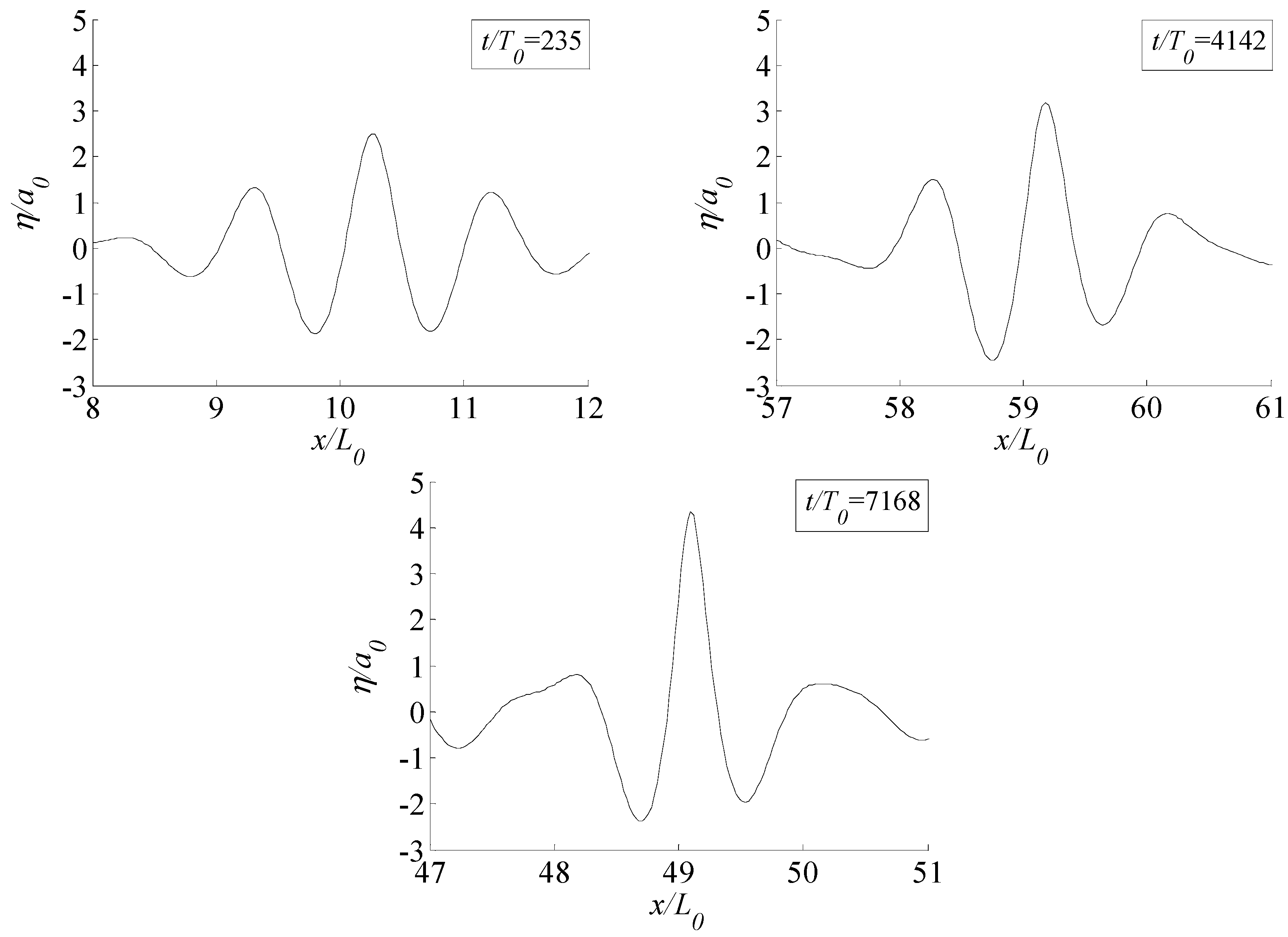
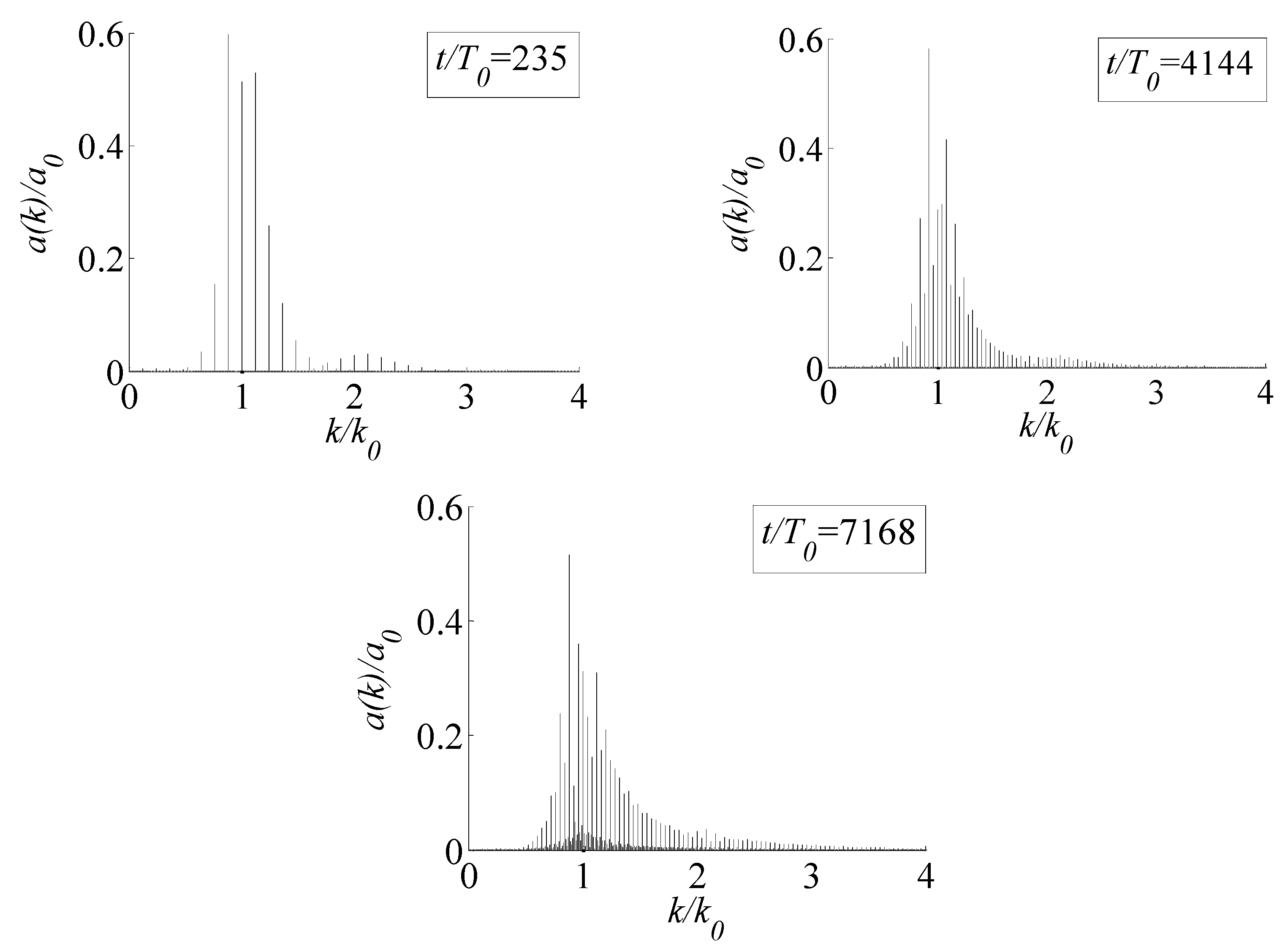
In this study, the nonlinear order of long-time evolution simulation of weakly modulated wave train is M = 7. In the case of initial carrier wave steepness ${\epsilon }_0=0.06$, the time scale of which modulated instability dominants in modulated Stokes wave train evolution is $t/T_0\approx O\left({\epsilon }_0{}^{-3}\right)\approx 4630$. The evolution process can be divided into three different time scales: $t/T_0\in \left[0,4000\right)$ $t/T_0\in \left[4000,7000\right]$.$t/T_0\in \left(7000,10\text{,}000\right]$, corresponding to the dominant stage of modulation instability, the transition stage, and the later stage of $t/T_0=O({\epsilon }_0^{-3})~2O({\epsilon }_0^{-3})$. Three moments corresponding to the occurrence of the maximum Freak wave in the above three different time scales under the condition of nonlinear order M = 7 is obtained by piecewise calculation, which are $t/T_0=235$, $t/T_0=4142$, $t/T_0=7168$, respectively. And

Table 2. Water particle velocity parameters of the maximum wave at different time scales under the condition of M = 7.

$\mathit{t}/{\mathit{T}}_0$	${\mathit{H}}_{\mathit{f}}/{\mathit{a}}_0$	Horizontal Water Particle Velocity of the Wave Peaks $\mathit{u}/{\mathit{u}}_0$	Vertical Water Particle Velocity on the Left ${\mathit{w}}_1/{\mathit{w}}_0$	Vertical Water Particle Velocity on the Right ${\mathit{w}}_2/{\mathit{w}}_0$
235	4.32	2.73	2.28	2.24
4142	4.87	3.61	2.97	2.51
7168	6.32	5.37	3.77	3.32

Note: $H_f$ is the Freak wave height, here $H_f\ge 4a_0$ is used as the criterion of Freak wave.

shows the water particle velocity parameters of the maximum wave of these three different time scales.

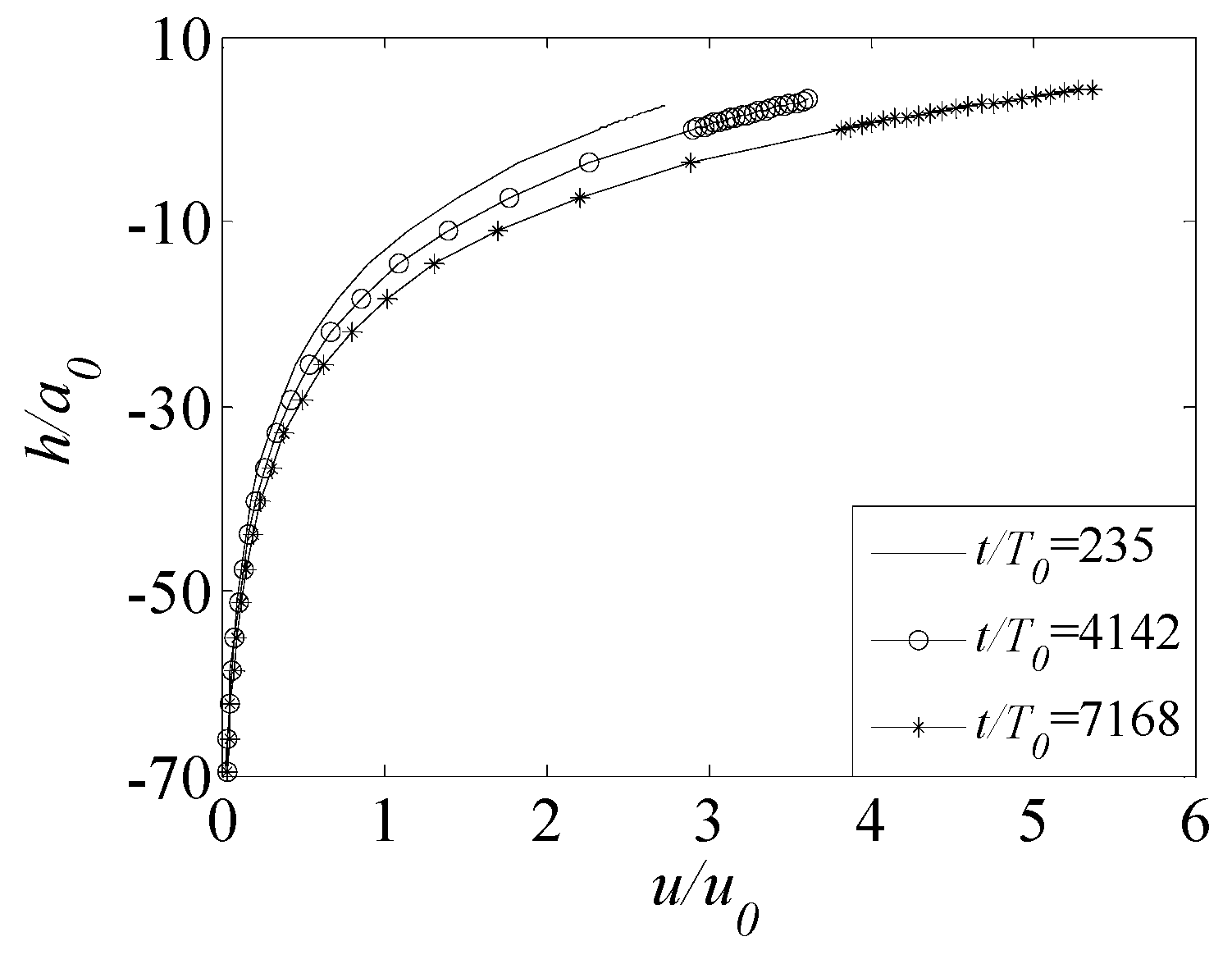
The variation of horizontal water particle velocity along with the water depth at the wave peak profile is shown in Figure 6. The dimensionless initial carrier amplitude $a_0=6\times {10}^{-4}$, and $u_0=w_0=6\times {10}^{-3}$.

It is found that the velocity of both sides of the wave peak is asymmetric. When the Freak wave is small, for example, in the dominant stage of modulation instability, the velocity difference between the left and right sides of the wave peak is not significant. With the enhancement of the Freak wave, the asymmetry of the velocity on both sides of the wave peak becomes more obvious. With the arrival of the wave peak, the water particle velocity of the wave peaks is exponential distribution along with the water depth. When the time of the wave train evolution is long enough, the nonlinear mechanism is stronger, the horizontal velocity of the water particles is larger, and reaches the maximum at the wave peak, which is consistent with the previous research results.

4.2. Extreme Value of Water Particle Velocity

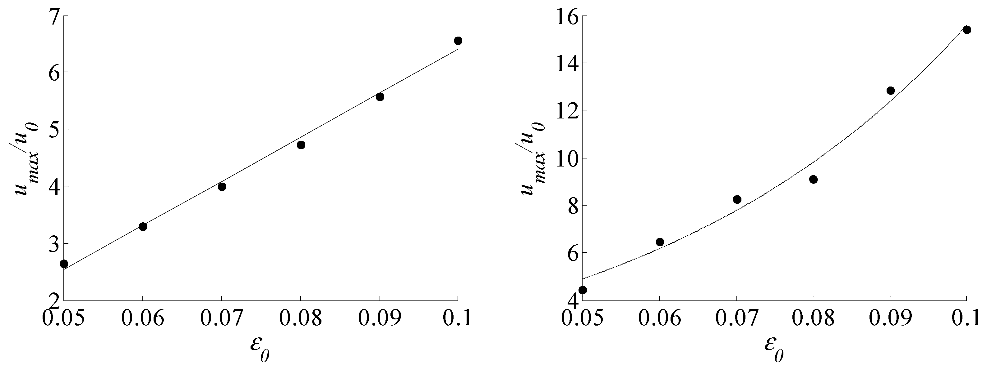
Under the condition of nonlinear order M = 7, taking $t/T_0=O\left({\epsilon }_0{}^{-3}\right)$ as the demarcation point, the relationship between the initial carrier wave steepness ${\epsilon }_0$ and the extreme water particle velocity of Freak wave peaks is shown in Figure 7. The ordinate is the dimensionless value $u_{\max }/u_0$ of the extreme value of the water particle velocity of Freak wave peaks and $u_0$ is the horizontal component of the dimensionless initial water particle velocity at the still water surface under the condition of the minimum wave steepness ${\epsilon }_0=0.05$, which is $5\times {10}^{-3}$ according to Formula (5).

Before the time scale $t/T_0=O\left({\epsilon }_0{}^{-3}\right)$, it is the dominant stage of modulation instability. There is a linear relationship between the extreme value of water particle velocity and the carrier wave steepness in this stage. The fitting formula is shown in Equation (7), and the correlation coefficient is 0.99. After the time scale $t/T_0=O\left({\epsilon }_0{}^{-3}\right)$, a new nonlinear mechanism appears, and the scope of study here is unified as $t/T_0=O({\epsilon }_0{}^{-3})~2O({\epsilon }_0{}^{-3})$, there is an exponential relationship between them. The fitting formula is shown in Equation (8), and the correlation coefficient is 0.98. It can be seen that in the modulation instability stage, the maximum water particle velocity of Freak wave peaks increases approximately linearly with the increase of wave steepness, while in the later stage, it exceeds the dominant stage of modulation instability, and a more complex nonlinear mechanism appears, which makes the maximum water particle velocity increases faster and faster with the increase of initial wave steepness.

$$u_{\max }/u_0=77.43{\epsilon }_0-1.338$$

(7)

$$u_{\max }/u_0=1.535\times e^{23.18{\epsilon }_0}$$

(8)

5. Influencing Factors of Water Particle Velocity

5.1. Wave Height

The relationship between horizontal water particle velocity of the wave peaks and wave height is studied in the initial condition of weakly modulation wave train. Three groups of realizations with initial wave steepness ${\epsilon }_0=0.05,0.07,0.09$ are selected, and the evolution time scales are $t/T_0=20\text{,}000;10\text{,}000;8000$.

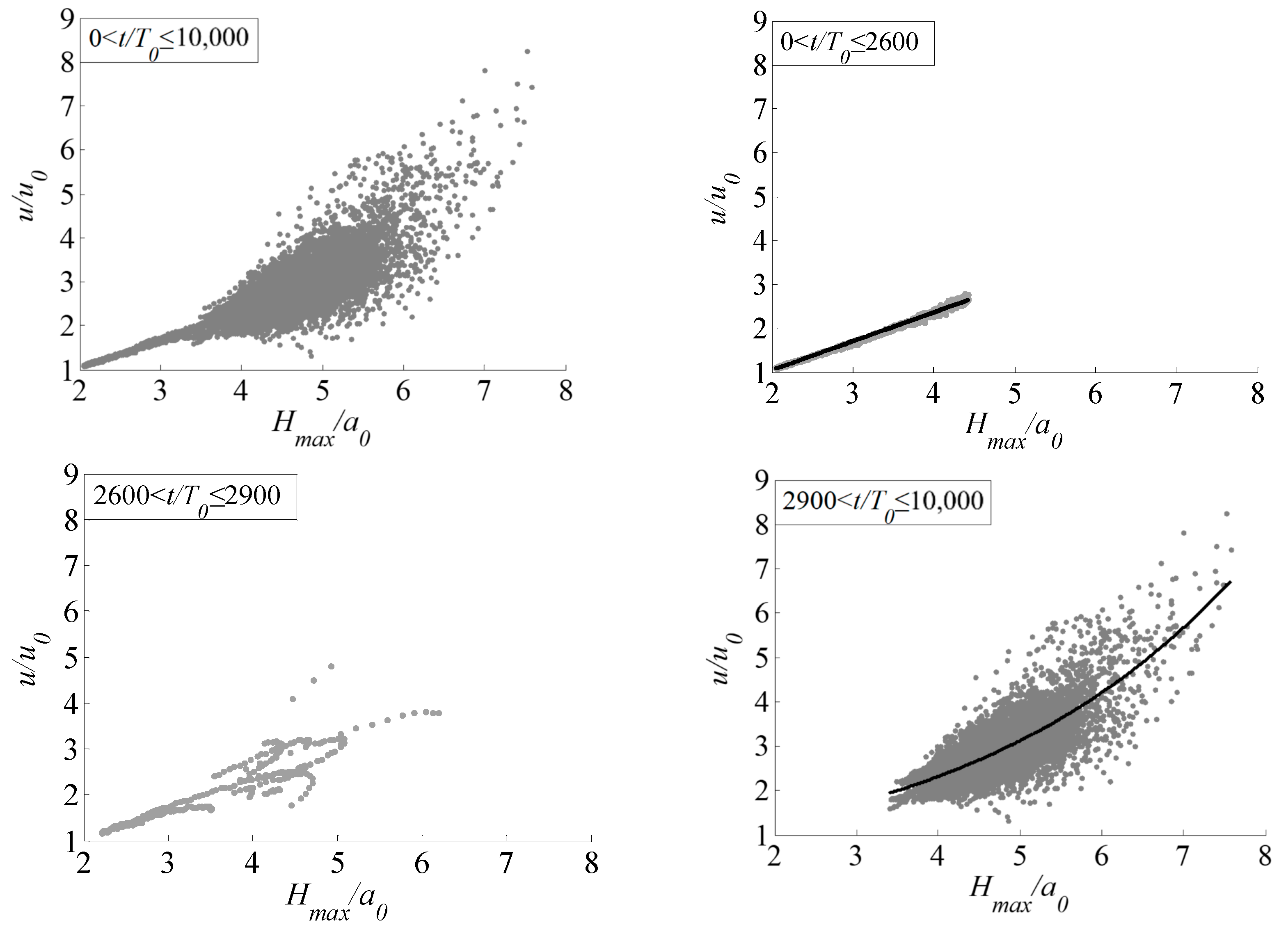
Taking the initial carrier wave steepness ${\epsilon }_0=0.07$ as an example, the relationship between the wave peak water particle velocity and wave height is explained in detail, as shown in Figure 8. The abscissa is represented by the dimensionless value of the maximum wave height in each period, denoted as $H_{\max }/a_0$, and the ordinate is represented by the corresponding dimensionless value of the wave peak water particle velocity, denoted as $u/u_0$, $a_0$ and $u_0$ are the computation space dimensionless initial carrier amplitude and the horizontal components of dimensionless initial water particle velocity at still water surface, respectively. $a_0$ is $7\times {10}^{-4}$ and $u_0$ is $7\times {10}^{-3}$ under the condition of ${\epsilon }_0=0.07$.

It can be found that the relationship between water particle velocity and wave height is different at different time scales. It can be divided into three stages to consider: The phase of modulation instability (before time scale $t/T_0\approx O({\epsilon }_0{}^{-3})$, it is taken as $0<t/T_0\le 2600$ here), there is a linear relationship between water particle velocity and wave height. The nonlinear characteristics are weak hear. Therefore, with the increase of wave height, the water particle velocity of the wave peaks still increases linearly. The relational expression $u/u_0=0.659\times H_{\max }/a_0-0.273$ is given, the correlation coefficient is 0.99. After time scale $t/T_0\approx O({\epsilon }_0{}^{-3})$, it is taken as $2900<t/T_0\le 10\text{,}000$), there is an exponential relationship between them. At this time, the nonlinear characteristics are stronger. With the increase of wave height, the water particle velocity of the wave peaks increases faster and faster. The relational expression $u/u_0=0.700\times e^{0.299H_{\max }/a}{}^{{}_0}$ is given, and the correlation coefficient is 0.60. There is a short transitional stage between these two times scales, in which the relationship between them is vague.

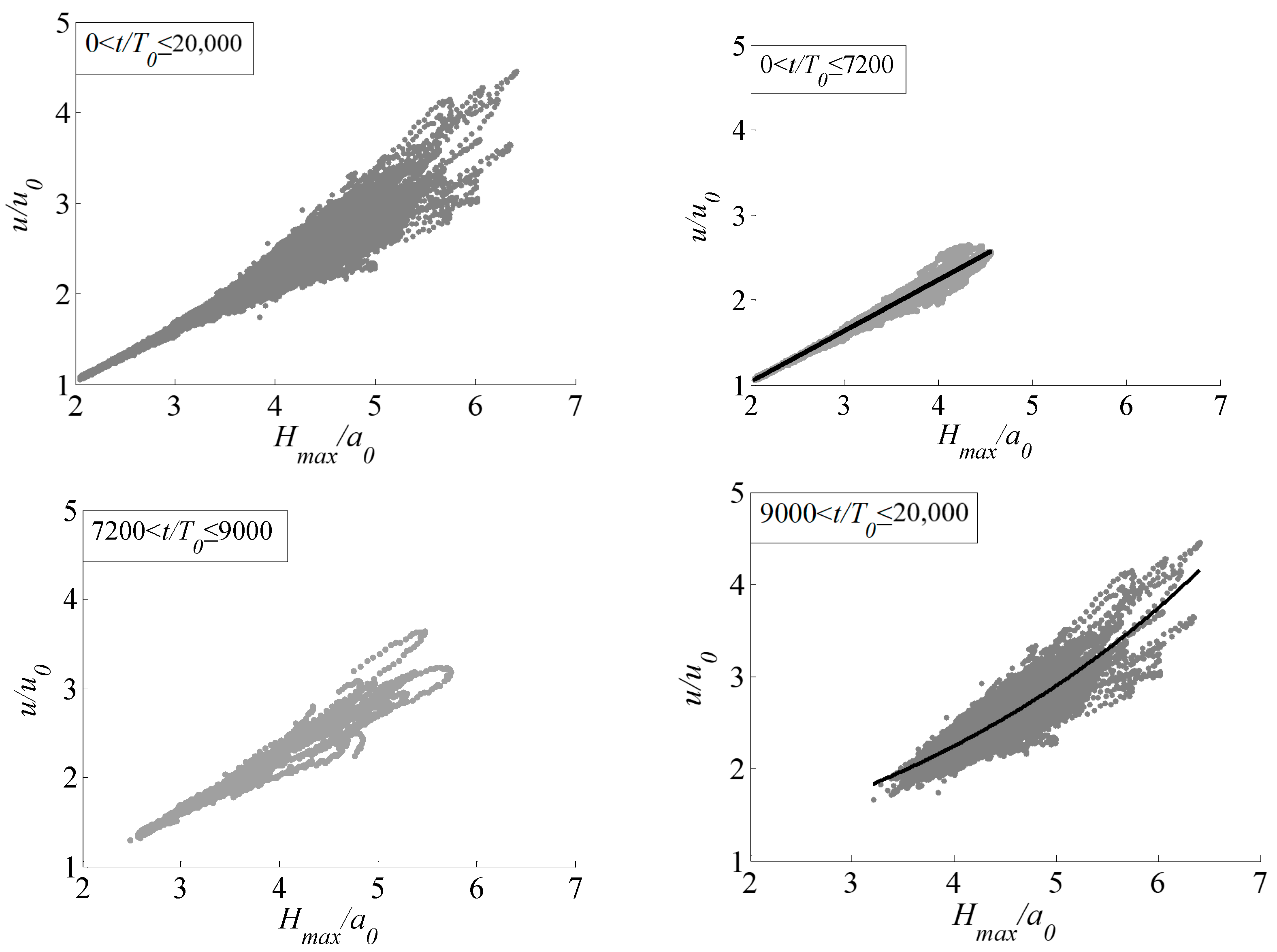
Similar results are obtained under the conditions of ${\epsilon }_0=0.05$ and ${\epsilon }_0=0.09$. When ${\epsilon }_0=0.05$, $a_0=5\times {10}^{-4}$, $u_0=5\times {10}^{-3}$, the relationship between water particle velocity of the wave peaks and wave height is shown in Figure 9. In the first stage, the time scale is $0<t/T_0\le 7200$, there is a linear relationship between them, expressed as $u/u_0=0.600\times H_{\max }/a_0-0.164$, and the correlation coefficient is 0.98. In the third stage, the time scale is $9000<t/T_0$ 20,000, the relationship between them is exponential, expressed as $u/u_0=0.807\times e^{0.256H_{\max }/a_0}$ with a correlation coefficient of 0.76. However, due to the small initial wave steepness, the relationship between them can also be considered linear. In the transitional period between the two times scales, the relationship between them is also approximately linear.

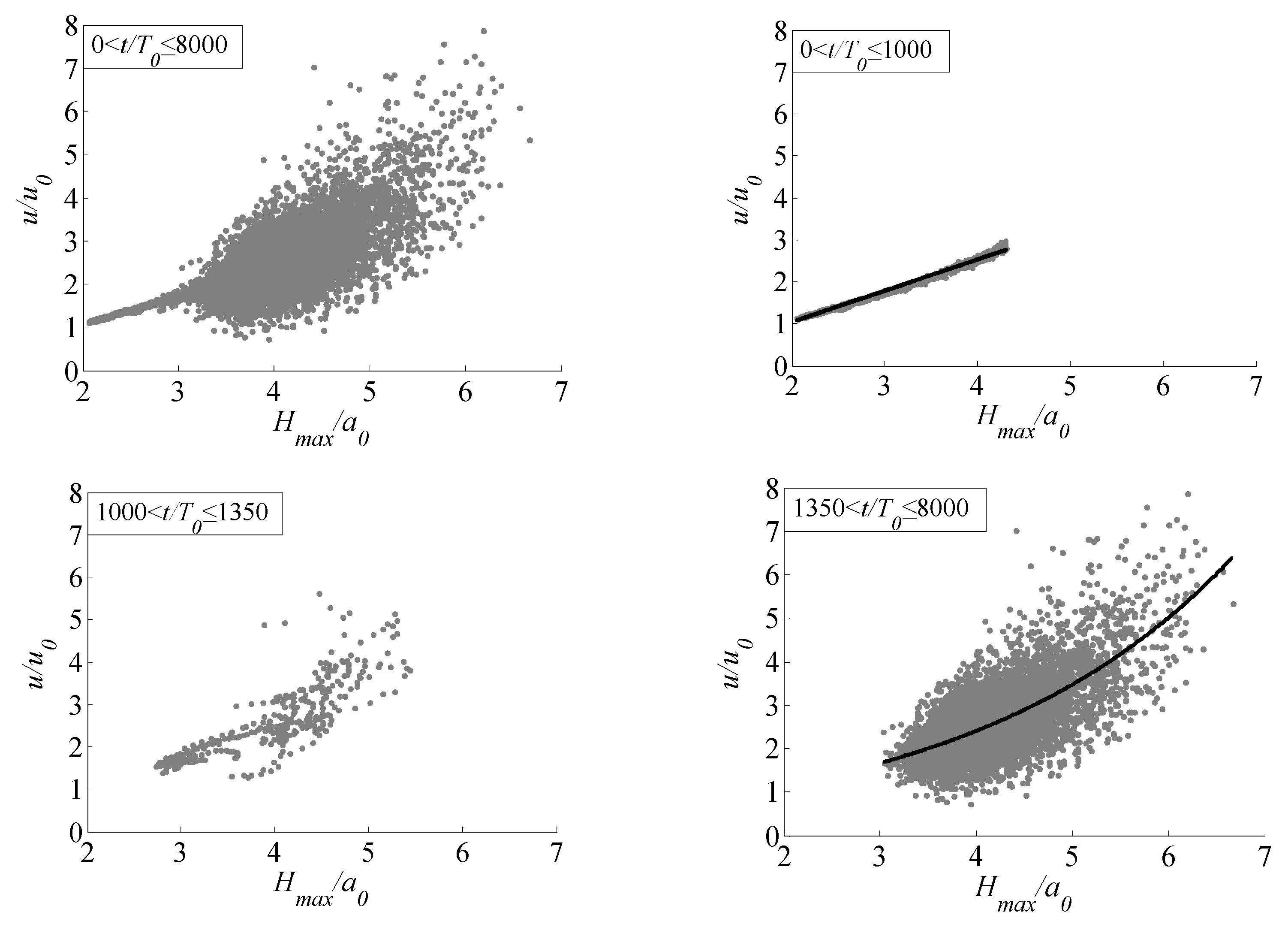
In the case of ${\epsilon }_0=0.09$,$a_0=9\times {10}^{-4}$, $u_0=9\times {10}^{-3}$.

Figure 10 shows the relationship between the water particle velocity of the wave peaks and wave height. In the first stage, the relationship is linear, the linear expression is $u/u_0=0.746\times H_{\max }/a_0-0.452$, the correlation coefficient is 0.99. In the third stage, there is an exponential relationship between them, expressed as $u/u_0=0.554\times e^{0.367H_{\max }/a}{}^{{}_0}$, the correlation is relatively weak. Similarly, there is a transitional stage $1000<t/T_0\le 1350$ in the middle, and the relationship between them is indistinct.

Therefore, the relationship between the water particle velocity of the wave peaks and wave height is closely related to the evolution time scale for different initial carrier wave steepness ${\epsilon }_0$ under the initial condition with weakly modulation wave train. The relationship between them is gradually divergent, from linear to exponential. When the initial wave steepness is small, the exponential relationship between them is weak and close to linear in the later stage.

5.2. Deformation Degree

In three groups of examples of the weakly modulated initial wave train, taking their respective maximum modulation wave height as the standard, the wave whose wave height is approximately equal to the maximum modulation time wave height is selected from the maximum wave height of each period in a given calculation period, to analyze the difference of Freak wave motion characteristics under two different nonlinear mechanisms. The screening wave height of each group is different, which is related to the initial wave steepness.

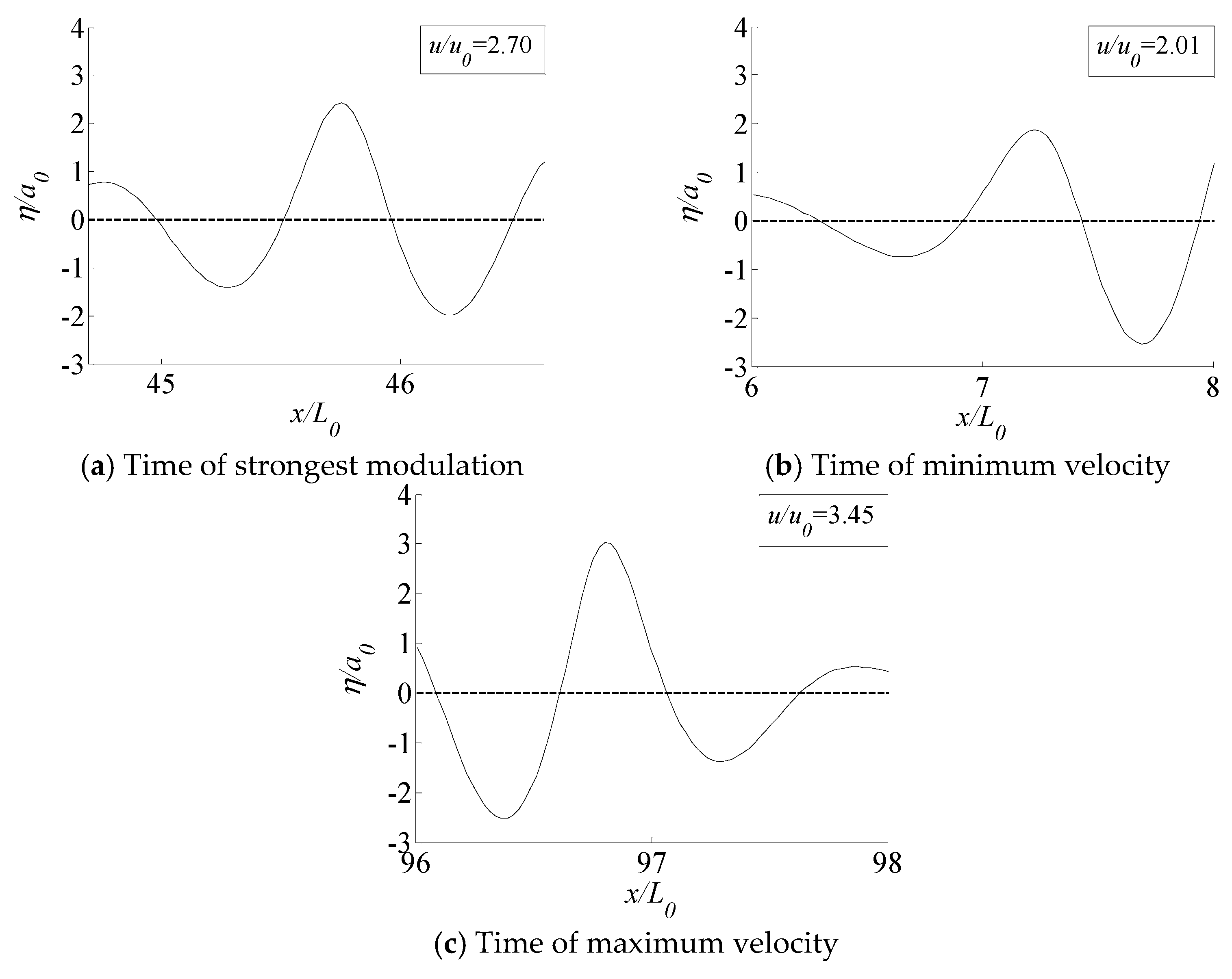
In the case of ${\epsilon }_0=0.07$, the wave height of maximum modulation time is about $4.41a_0$, taking $4.40a_0\le H_j\le 4.42a_0$ as the screening standard, 172 groups of Freak waves which are approximately equal to the maximum modulation time wave height, are screened out in 10,000 periods. There are significant differences in the water particle velocity of the wave peaks of these Freak waves. The waveforms at the strongest modulation time and the following two times with large differences in wave velocity are given for further comparison, as shown in Figure 11.

Figure 11 shows that when the wave heights are similar, the shapes and contours of the Freak waves corresponding to different generation mechanisms are different. The difference is mainly manifested in the different horizontal symmetry of the waveforms. One is that the amplitude of the maximum modulation wave surface is more than twice of the initial carrier wave amplitude, and the height of the wave peak η_c is higher than the depth of the wave trough η_t, that is to say, it shows obvious nonlinear characteristics, researchers call this nonlinear feature deformation degree. The deformation degree is introduced and defined as Equation (4). It may be the main reason for the difference in the water particle velocity of the wave peaks. In the stage of modulation instability, the shapes of the Freak waves at the strongest modulation moment are the same, showing that the peaks are slightly larger than the troughs. While after $t/T_0\approx O({\epsilon }_0^{-3})$, the deformation degree of waveform changes significantly—some become larger, some become smaller—and the water particle velocities of Freak waves that have larger deformation degrees, are larger. Try to fit the relationship between water particle velocity of the wave peaks and deformation degree $\gamma$ under the condition of similar wave height, as shown in Figure 12, the relationship is linear, the relational expression is $u/u_0=5.504\gamma -0.352$, the correlation coefficient is 0.96.

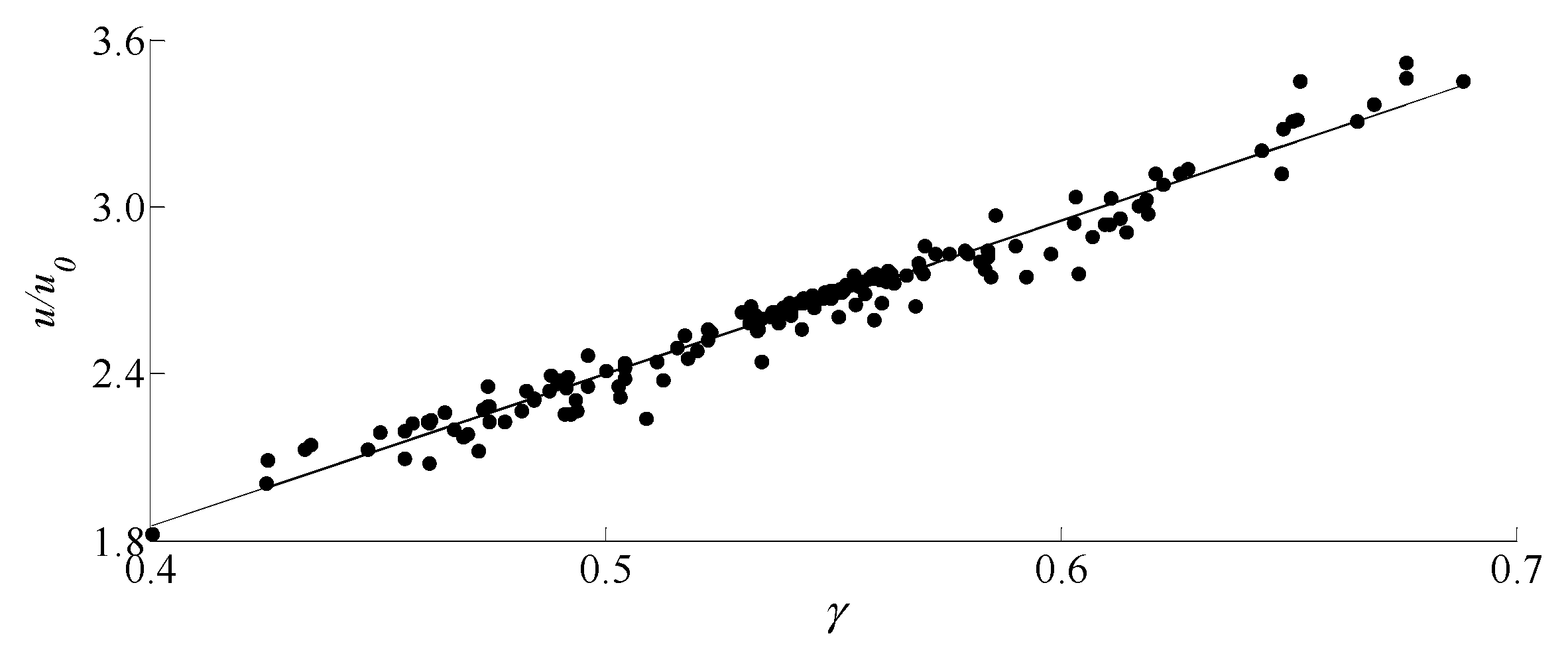
Similarly, when ${\epsilon }_0=0.05$ and ${\epsilon }_0=0.09$, we repeated that treatment. When ${\epsilon }_0=0.05$, the wave height of maximum modulation time is about $4.54a_0$. A total of 233 groups of wave heights approximately equal to it are screened out in 20,000 calculation periods, and the screening standard is $4.53a_0\le H_j\le 4.55a_0$. Under the condition of similar wave height, the correlation between water particle velocity of the wave peaks and deformation degree $\gamma$ is $u/u_0=5.167\gamma -0.155$, and the correlation coefficient is 0.98.

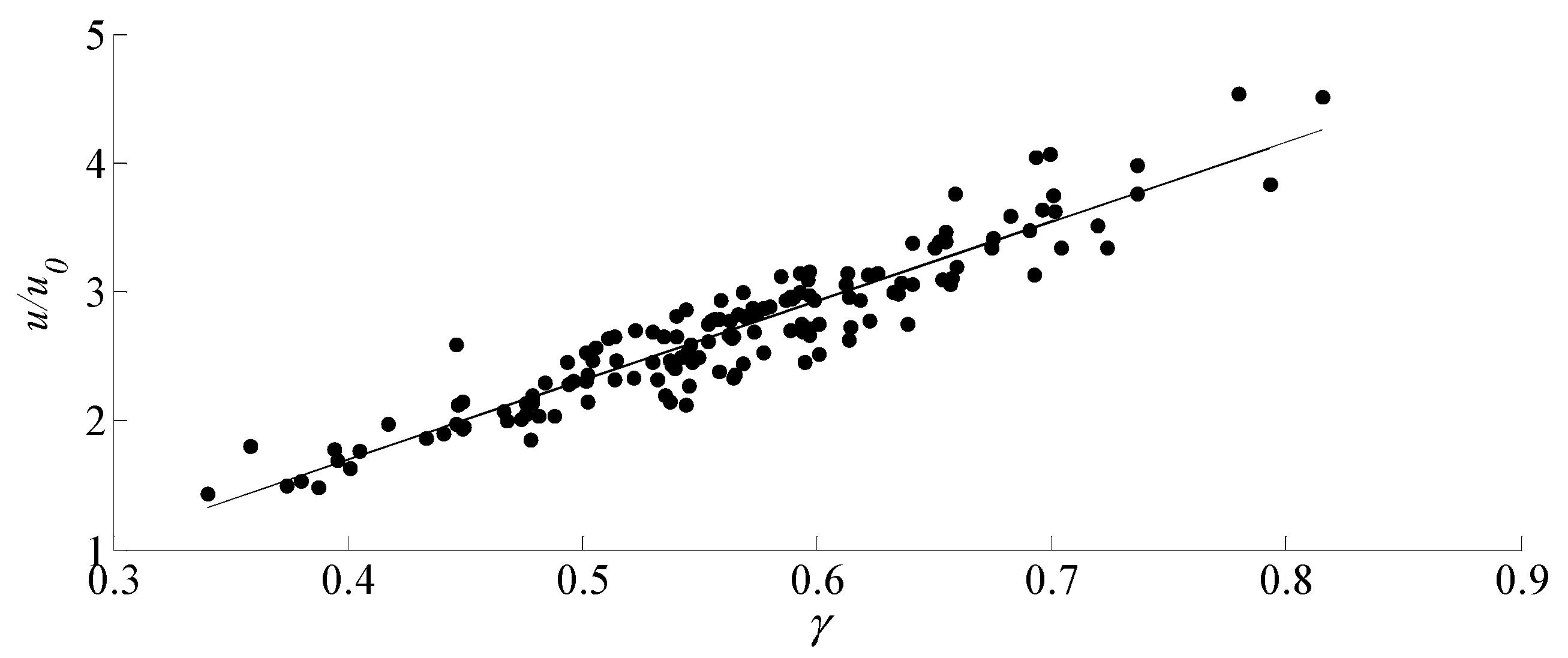
When ${\epsilon }_0=0.09$, the wave height of maximum modulation time is about $4.30a_0$. A total of 151 groups of wave heights approximately equal to $4.30a_0$ are screened out in 8000 calculation periods, and the screening standard is $4.29a_0\le H_j\le 4.31a_0$. Under the condition of similar wave height, the relationship between water particle velocity of the wave peaks and deformation degree $\gamma$ is $u/u_0=6.146\gamma -0.759$, and the correlation coefficient is 0.87. The results are shown in Figure 13 and Figure 14, respectively.

In summary, under the condition of similar wave height, the most important factor affecting the water particle velocity is deformation degree. Different generation mechanisms lead to different deformation degrees of Freak waves, which lead to different wave peak heights, resulting in the difference of water particle velocity of the wave peaks. Under the background of similar wave height, the smaller the initial wave steepness, the higher the linear correlation between deformation degree and water particle velocity of the wave peaks. With the increase of the initial wave steepness, the linear correlation weakens. It is reasonable to speculate that when the initial wave steepness is larger, other factors affecting the water particle velocity may appear.

5.3. Wave Peak Height

From the above analysis, we can see that the most important factor of water particle velocity in a similar wave height is deformation degree, that is, the water particle velocity of the wave peaks is closely related to the wave peak height.

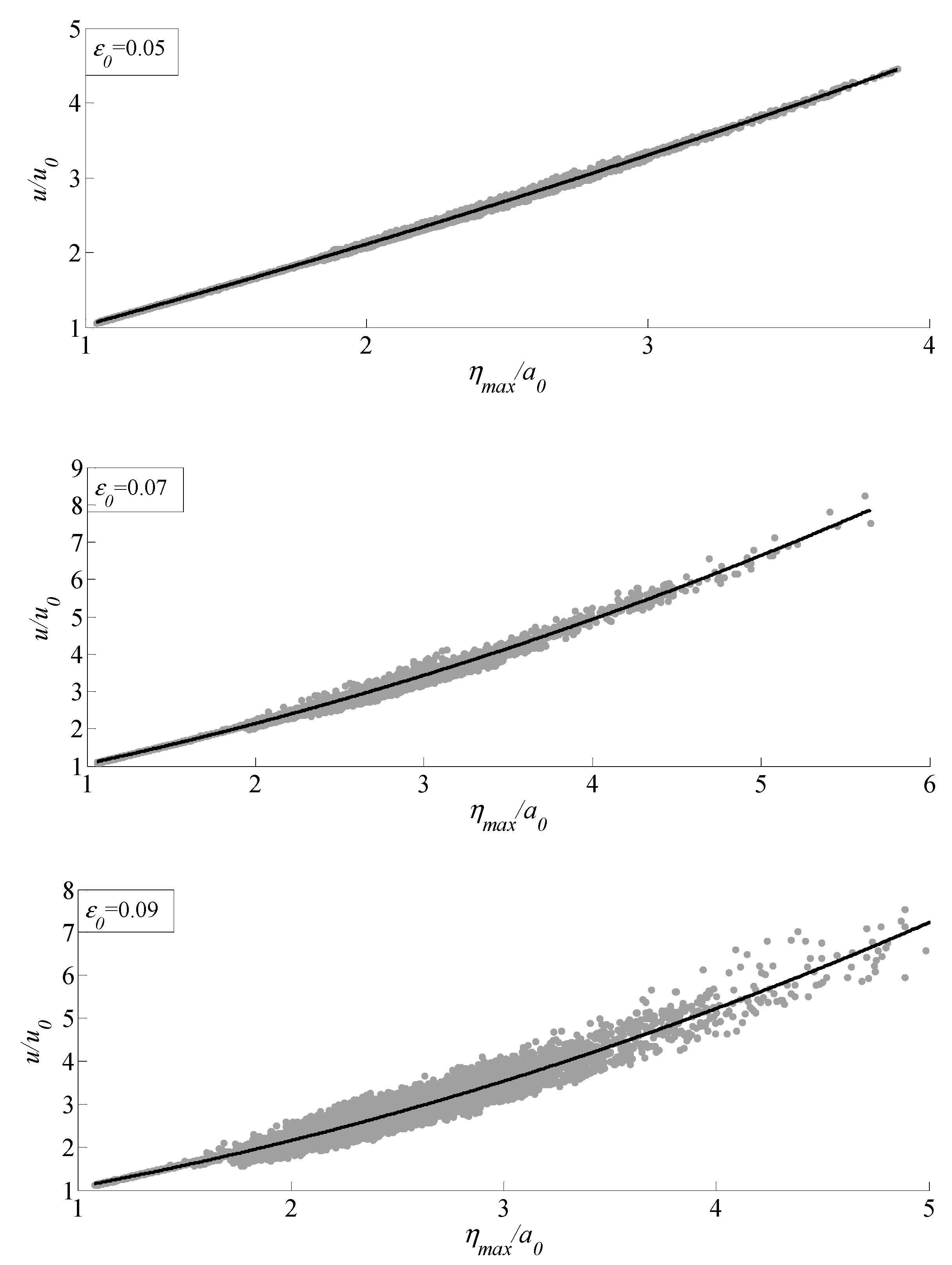
Under the initial condition of a weakly-modulated wave train, the relationship between water particle velocity and wave peak height under different initial wave steepness conditions is given, as shown in Figure 15. It can be found that there is a quadratic function relationship between the water particle velocity and the peak height. When the initial carrier wave steepness is ${\epsilon }_0=0.05$, the relationship between them is shown in Equation (9), and the correlation coefficient is almost equal to 1. When the initial carrier wave steepness is ${\epsilon }_0=0.07$, the relationship between them is shown in Equation (10), and the correlation coefficient is 0.98. When ${\epsilon }_0$ is increased to 0.09, the relationship between them is shown in Equation (11), and the correlation coefficient is 0.93. It can be found that with the increase of the initial wave steepness, the coefficient of the second-order term increases gradually, which indicates the increase of the level of nonlinearity.

$$u/u_0=0.0541\times {\eta }_{\max }/a_0{}^2+0.921\times {\eta }_{\max }/a_0+0.0528$$

(9)

$$u/u_0=0.105\times {\eta }_{\max }/a_0{}^2+0.766\times {\eta }_{\max }/a_0+0.188$$

(10)

$$u/u_0=0.155\times {\eta }_{\max }/a_0{}^2+0.608\times {\eta }_{\max }/a_0+0.315$$

(11)

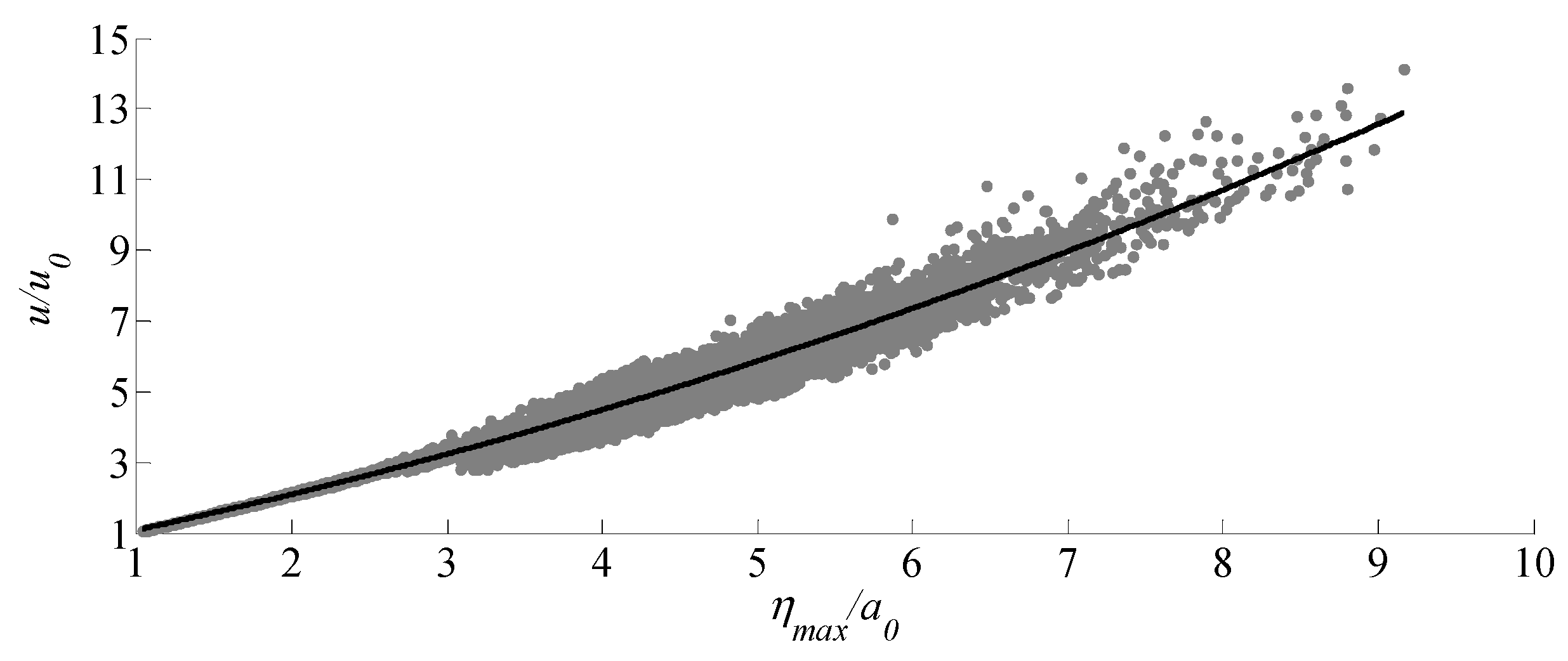
We try to uniformly express the relationship between the wave peak height and water particle velocity of the weakly modulated wave train with different initial wave steepness ${\epsilon }_0$. Here, two groups of wave steepnesses ${\epsilon }_0=0.06,0.08$ are added, and the evolution time is $t/T_0=10\text{,}000$, the data of 5 groups are combined. $a_0$ and $u_0$ are the dimensionless initial carrier amplitude and the horizontal components of dimensionless initial water particle velocity at still water surface when ${\epsilon }_0=0.05$, respectively. $a_0=5\times {10}^{-4}$ and $u_0=5\times {10}^{-3}$. The results are shown in Figure 16. Then the relationship between them can be expressed by Equation (12), the correlation coefficient is 0.98.

$$u/u_0=0.0606\times {\eta }_{\max }/a_0{}^2+0.829\times {\eta }_{\max }/a_0+0.192$$

(12)

Therefore, for the weakly-modulated initial wave train, the relationship between water particle velocity and wave peak height can be described uniformly under different initial wave steepness conditions, and the water particle velocity can be calculated from the wave peak height. When ${\epsilon }_0$ is smaller, the correlation between them is almost linear with the ratio of 1. At this time, it can be considered that the water particle velocity is consistent if the wave peak height is consistent. While ${\epsilon }_0$ is larger, the correlation between the two becomes weaker, especially as the peak height increases, the relationship between them gradually becomes divergent. At this time, due to the strong nonlinear effect, there may be other factors that affect the water particle velocity.

5.4. Sharpness of the Wave Peaks

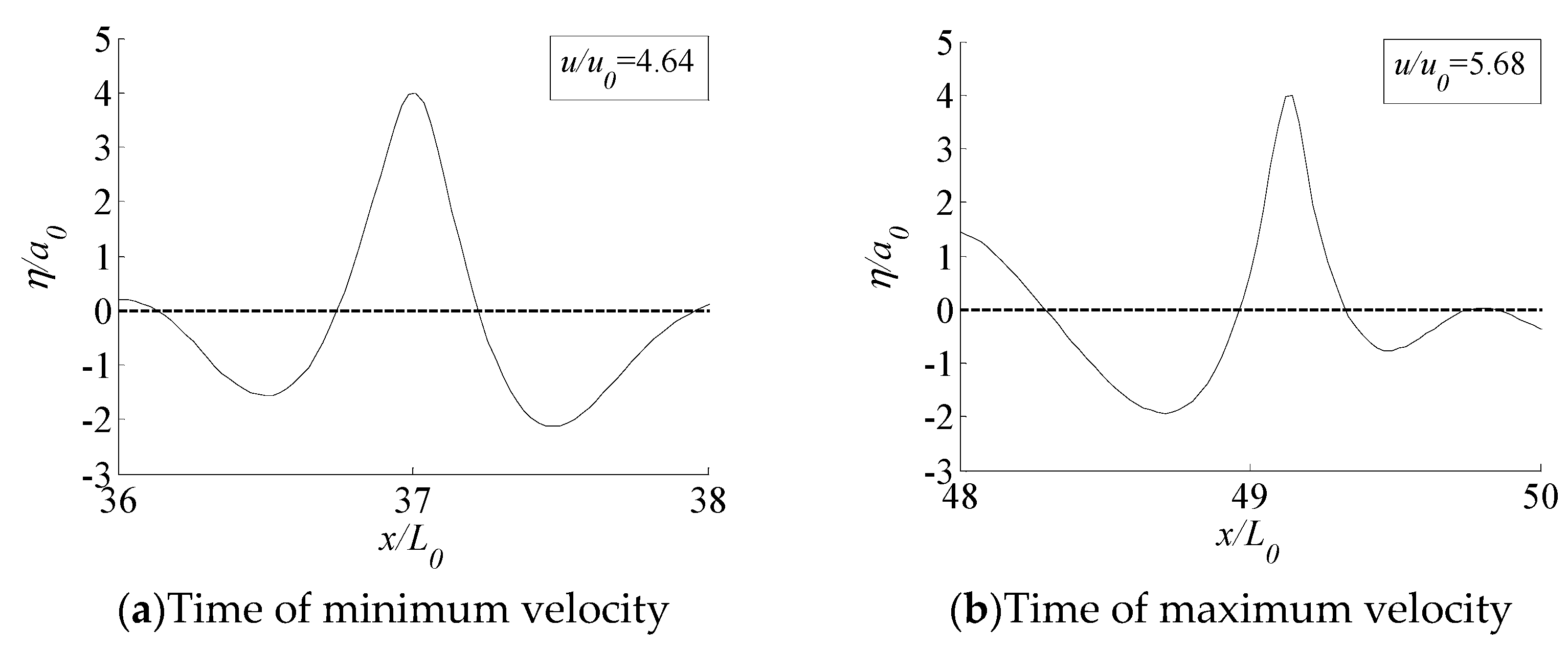
It can be seen from the above that when the initial carrier wave steepness of the weakly modulated wave train is large, there are other factors that affect water particle velocity of wave peak besides the wave peak height. Then, for the initial condition with weakly modulated wave train, the case where the initial carrier wave has a steep steepness ${\epsilon }_0=0.09$ is studied, and the waveforms with significant differences between the two wave velocities whose peak heights are both $4a_0$ are shown in Figure 17.

In this case, when the wave peak heights are similar, it is obvious that the difference of waveforms of Freak waves which have great differences in water particle velocities is also great, which is manifested by different sharpness of wave peak. When the wave peak is sharper, the corresponding wave peak water particle velocity is also larger. For the initial weakly-modulated wave train, the effect of peak sharpness on water particle velocity only appears when ${\epsilon }_0$ is large.

6. Conclusions

In this study, based on the initial condition with weakly-modulated wave train, the characteristics of water particle velocity of Freak waves generated by nonlinear self-focusing mechanisms are studied and analyzed. And several conclusions are as follows.

(1)

The water particle velocities of Freak waves are asymmetrical on both sides of the wave peak, the longer the evolution time is, the stronger the nonlinearity we consider. At this time, the Freak wave is larger, and the asymmetry of velocity is more obvious. The horizontal water particle velocity reaches the maximum at the peak and varies exponentially along with the water depth.

(2)

In the stage of modulation instability, the extreme value of water particle velocity of the wave peaks increase linearly with the initial wave steepness ${\epsilon }_0$. In the later stage $t/T_0=O({\epsilon }_0{}^{-3})~2O({\epsilon }_0{}^{-3})$, the stronger nonlinear mechanism appears, it increases exponentially with the initial wave steepness ${\epsilon }_0$.

(3)

For the initial wave train of weakly-modulated, the water particle velocity of the wave peaks and wave height show a linear relationship in the stage dominated by modulation stability, and exponential in the stage of $t/T_0=O({\epsilon }_0{}^{-3})~2O({\epsilon }_0{}^{-3})$. There is a transitional phase between the two dominant phases of different mechanisms.

(4)

When Freak waves are similar in wave height, the different deformation degrees of Freak waves result in the difference of water particle velocity of the wave peak, and the water particle velocity of Freak waves with larger deformation degree is larger.

(5)

The relationship between the water particle velocity of the wave peaks and wave peak height is a quadratic function. This relationship is better when the initial carrier wave steepness ${\epsilon }_0$ is small. When ${\epsilon }_0$ increases, the sharpness of the Freak wave peak also becomes an important factor affecting the water particle velocity of the wave peak, and the water particle velocity increases with the sharpness of the wave peak for the similar wave peak height.