3. The Mathematics of a Continuous Evanescent Pressure Field
Most available mathematics use continuous waves with no start time that extend throughout all space, but yield convenient mathematical forms such as the sine wave. They can be compared to excitation by an impulse, such as that used for our computer modeling. The mathematical nature of these pressure fields was discussed by Fahy [
21]. He showed that when the speed of the solid wave is less than that of the pressure wave in the adjacent fluid, there will be no radiation of energy from the plate into the fluid. The resultant exponential decay of the acoustic pressure with increasing distance from the plate is described as an evanescent field.
The decay can be described by a field thickness
δ. While both particle velocities and pressures decay at the same rate, it is convenient to consider the variation of the acoustic pressure,
p:
The pressure at the interface p0 will have dropped to a fraction 1/e when the distance from the interface z is equal to δ. This field thickness will vary with the oscillatory frequency and other parameters. This exponential decay is similar to the “skin effect” of electromagnetic theory.
The evanescent field thickness is proportional to the wavelength of the interface wave,
λ:
where
cw is the compressive water wave speed and
cd is the particle displacement interface wave speed. This equation has been reconfigured to use the wavelength, λ, from Fahy’s original, which used the wavenumber. When
cw >> cd, δ becomes close to
λ/2π, the inverse of the wavenumber,
k, for the wave being driven along the solid interface, is given by:
In Equation (3), Fahy’s wavenumber ratio has been replaced by a ratio of wave speeds. Since both waves have the same frequency, f, their ratio is the inverse of the wavenumber ratio.
4. Results from Transient Finite Element (FE) Modeling
4.1. The FE Graded Model
Unlike an infinite physical model, the FE mesh is finite. We created a set of elements by defining a data file of their properties for the computation. These small contiguous blocks had specified isotropic material properties, which were then subjected to small elastic deformations by the imposed force. These deformations were transmitted from element to element by a large number of elastic responses between the elements. The FE process is linear, in that if the force is doubled, all responses are also doubled. We thus used an arbitrary 1 MN peak force to generate realistic responses. A benefit of the transient analysis is the ability to use an impulsive excitation force. This has to be kept short in both time and space to avoid unwanted errors, but will track changes with time. We used a more flexible impulsive force for this work than those we used previously.
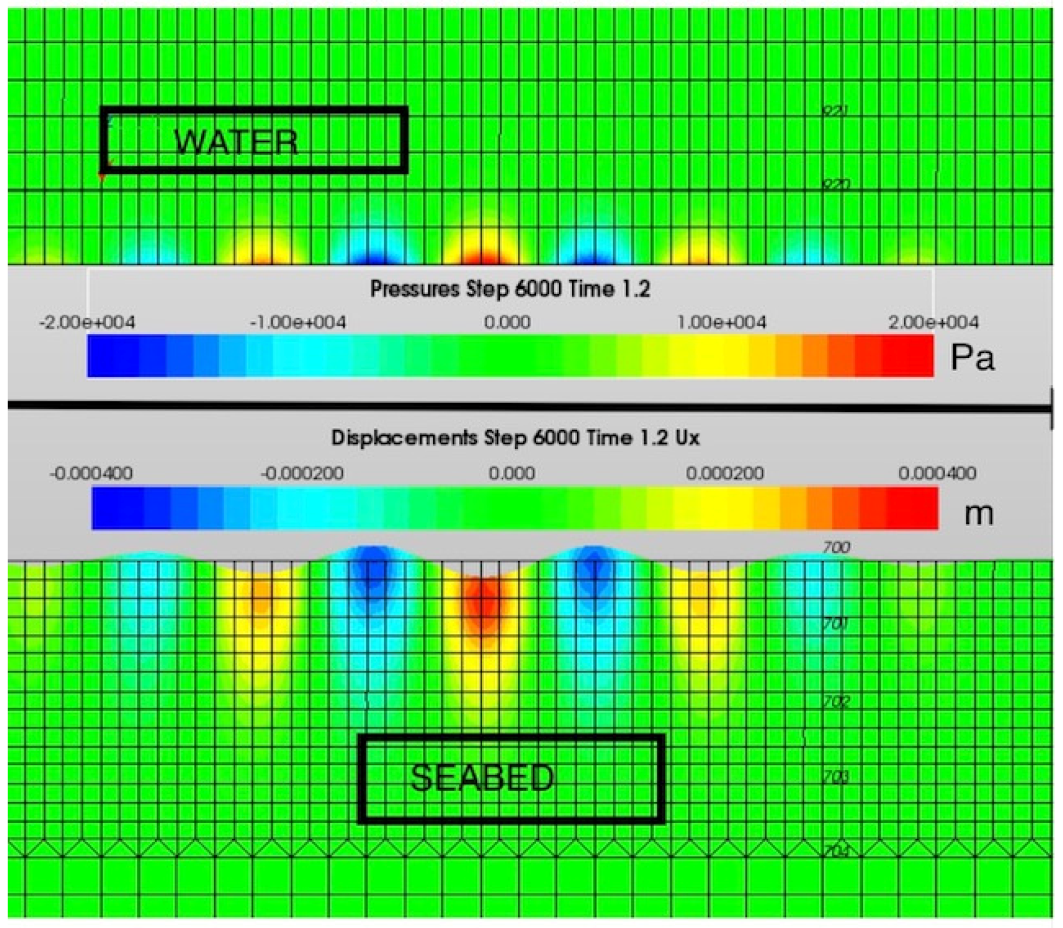
The FE model was a pair of stacked discs, shown in cross-section in
Figure 1. The lower disc was solid, with a depth usually specified as 128 m, of which just over 2 m is shown, but the disc radius varied, often set to 256 m. Many thousands of elements were defined, with the smaller elements shown by the grid in this figure being 0.125 m square. These needed to be kept small compared with the wavelength. By doing so, the discrete divisions between the elements had little effect, and the FE model could simulate the continuous variation in material properties of the physical model.
The displacement waves are shown by an exaggerated deformation of the interface. Here, five troughs or dips are shown with a wavelength of approximately 12 elements or 1.5 m. The upper disc is water, with a depth of 16 m, of which the lower 1.7 m is shown. Note that this model assumed axisymmetry, with no circumferential variation.
Defined points in the FE model are called nodes, corresponding to particles of solid or water. Node 700 is marked on the interface. This is halfway out from the centre at 128 m radius. Node 920 is within the water at 0.5 m above the interface. More effort was placed on the analysis of such nodes in this paper than in our previous work. The primary calculation for these acoustic elements is of the acoustic pressure, but postprocessing can be done to recover the water-particle motion.
4.2. The FE Layered Model
The layered physical model is more easily rendered by the FE technique, as the substrate layer is finite. Steel was used, with its well-defined material properties, but the mathematics will be similar for a rock layer.
The diameter was made large enough to be able to avoid confusion between the outgoing wave and the return after a reflection at the circumference. This FE model will be referred to as the tank model, representing a 16 m deep water tank of diameter 512 m with a 0.125 m thick steel base. Excitation forces were applied downward to the tank centre, using low frequencies (e.g.,16 Hz) to create an evanescent pressure field in the water near the bottom.
Although the motion of the steel plate was primarily vertical, the adjacent water motions retained the substantial horizontal velocities of the graded model. This indicated that these water-particle velocities were a consequence of the intrinsic fluid mechanics within the evanescent field, and were independent of the horizontal motion of the solid below. The fluid as modeled had no viscosity.
4.3. The Nature and Influence of the Energy Source
Both the graded and layered FE models were excited by a force applied as a downward thrust at the centre of the substrate disc. This was chosen to represent the actions of a pile driver or dredger. However, there was limited realism in this choice. The FE method had difficulty in modeling a cutting action. Both piling and dredging require the rupture of the seabed material, and this was outside the scope of this work. However, the elastic waves as modeled showed most features of the observed seabed vibrations, so we studied the propagation from the idealized thrust to the consequent motion.
The displacements of the particles as shown in
Figure 1 created two particle velocity components, described henceforth as upward and outward. In contrast, the applied thrust was only vertical, and applied to a point at the centre of the model. The horizontal velocities that were integral to the seismic interface wave structure were thus generated within the model, as the energy was converted from that of a vertical thrust into a two-dimensional velocity vector. There was no circumferential velocity in this axisymmetric model. This conversion process may have some similarity to the process that converts a fluctuating volume source (a “simple source” as described by Kinsler et al. [
22]) into a plane pressure wave within open water. This is usually described by comparing the simple physics of the near field to that of the far field, with a more complicated structure as the conversion proceeds.
4.4. The Energy-Source Time Profile
Our 2016 work used a polynomial variation of thrust with time over a defined period, designed to limit the acceleration values. For the 2018 work, this was changed to a Ricker pulse, an infinite pulse profile, with very low values at times well away from the peak. The profile was truncated at a time when the level was extremely low.
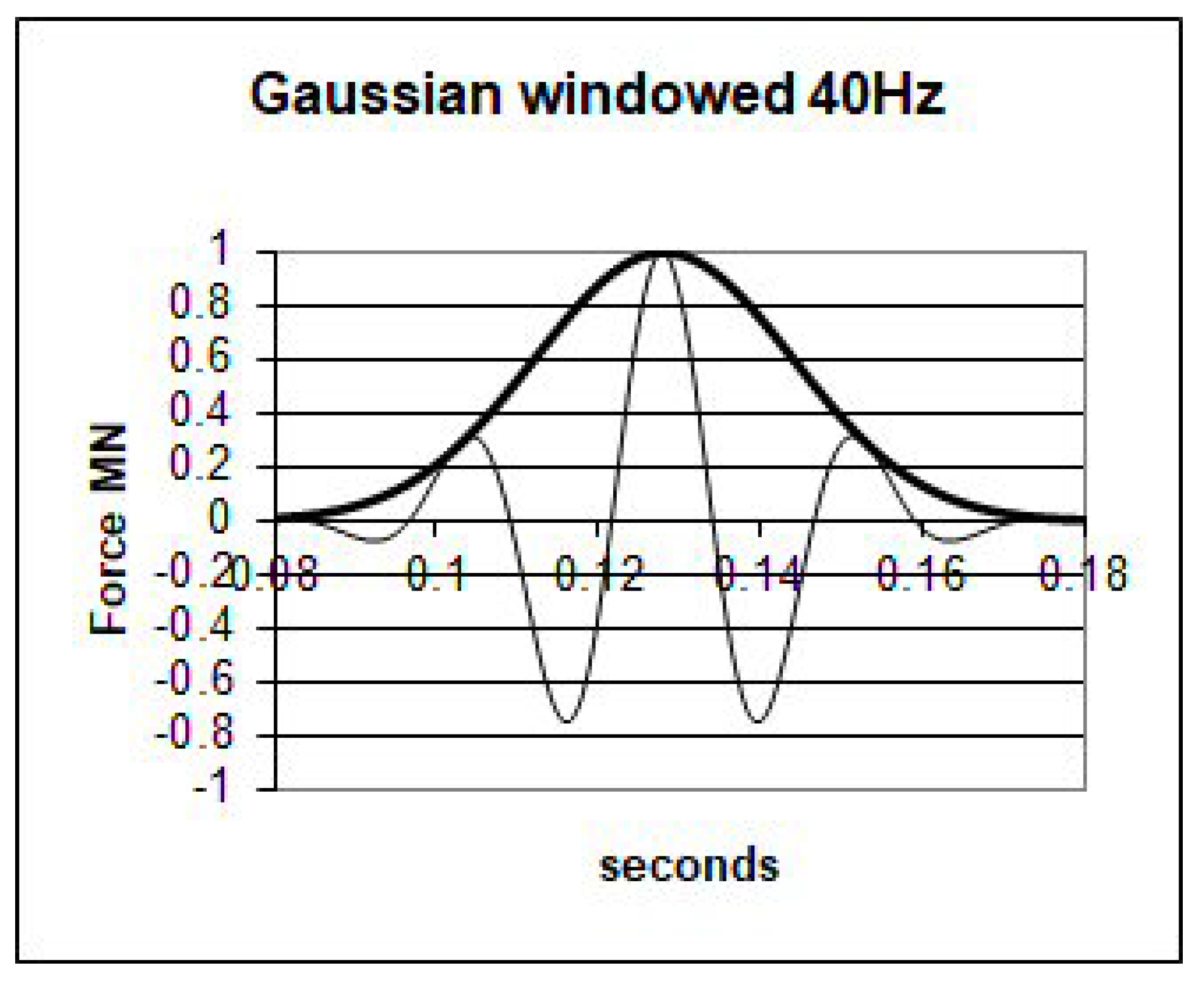
Both these pulse forms have been replaced in this work by a truncated windowed cosine form. The cosine form was windowed by a Gaussian “bell” curve, as seen in
Figure 2. In addition to the cosine frequency f, set here to 40 Hz, the bell curve was specified by a time width,
tw, and a peak time,
t0. The peak amplitude force
F was set at an arbitrary
K = 1 MN. Here, the window width
tw = 0.0226 s.
The envelope form is shown in
Figure 2 by the bold black line, while the applied force is shown by the lighter grey line. This improved impulse driver allowed the frequency of the propagated displacement wave to be set. However, it was not based on any measurements of piling action, but rather adopted to replicate features of the observed waveforms.
4.5. The Time Profile of the Response
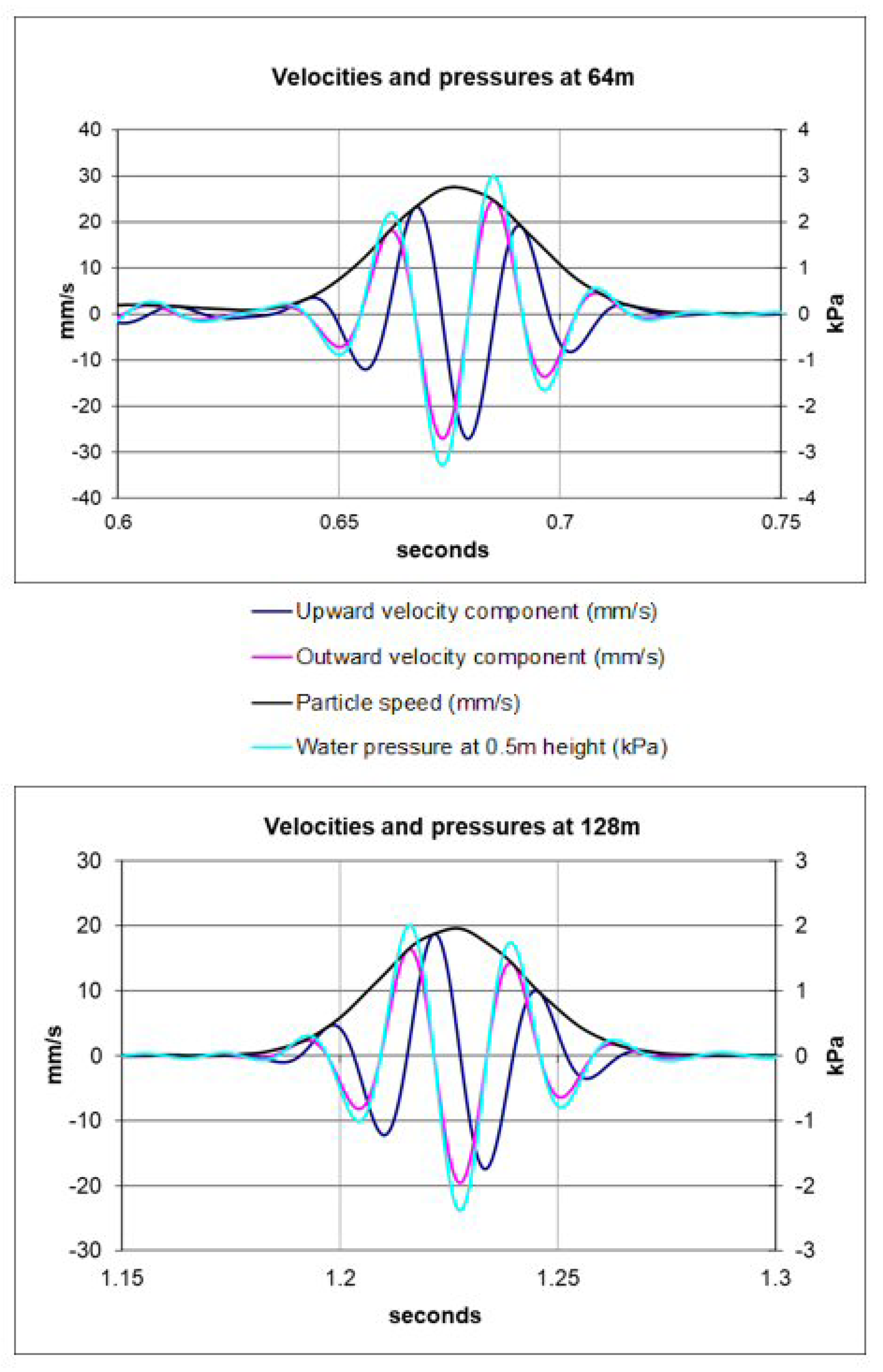
The form of the time response is shown in
Figure 3 at two positions, 64 m and 128 m from the centre of the model. The response at a radius of 128 m was taken at node 920, which is labeled in
Figure 1. The water-particle kinetic energy depended on the particle speed, a scalar found by combining the upward and outward velocity components.
Notably, it was the time profile of the particle speed that followed the form of the applied impulse window function, the envelope shape of the wave packet. This bell shape was seen to propagate unchanged from the node at radius 64 m to that at 128 m. In contrast, the individual velocity components of the displacement wave followed the more rapid oscillations of the applied force. At different positions, the peaks and troughs of the two components occurred at different times within the envelope. This was a consequence of the displacement wave speed being faster than the speed of the envelope. This behaviour is well documented for other branches of physics, in which they are referred to as the “phase velocity” and “group velocity”, respectively. These include ocean surface waves, controlled by gravity, where the wave structure is highly dispersive, with a characteristic ensuing chaotic motion.
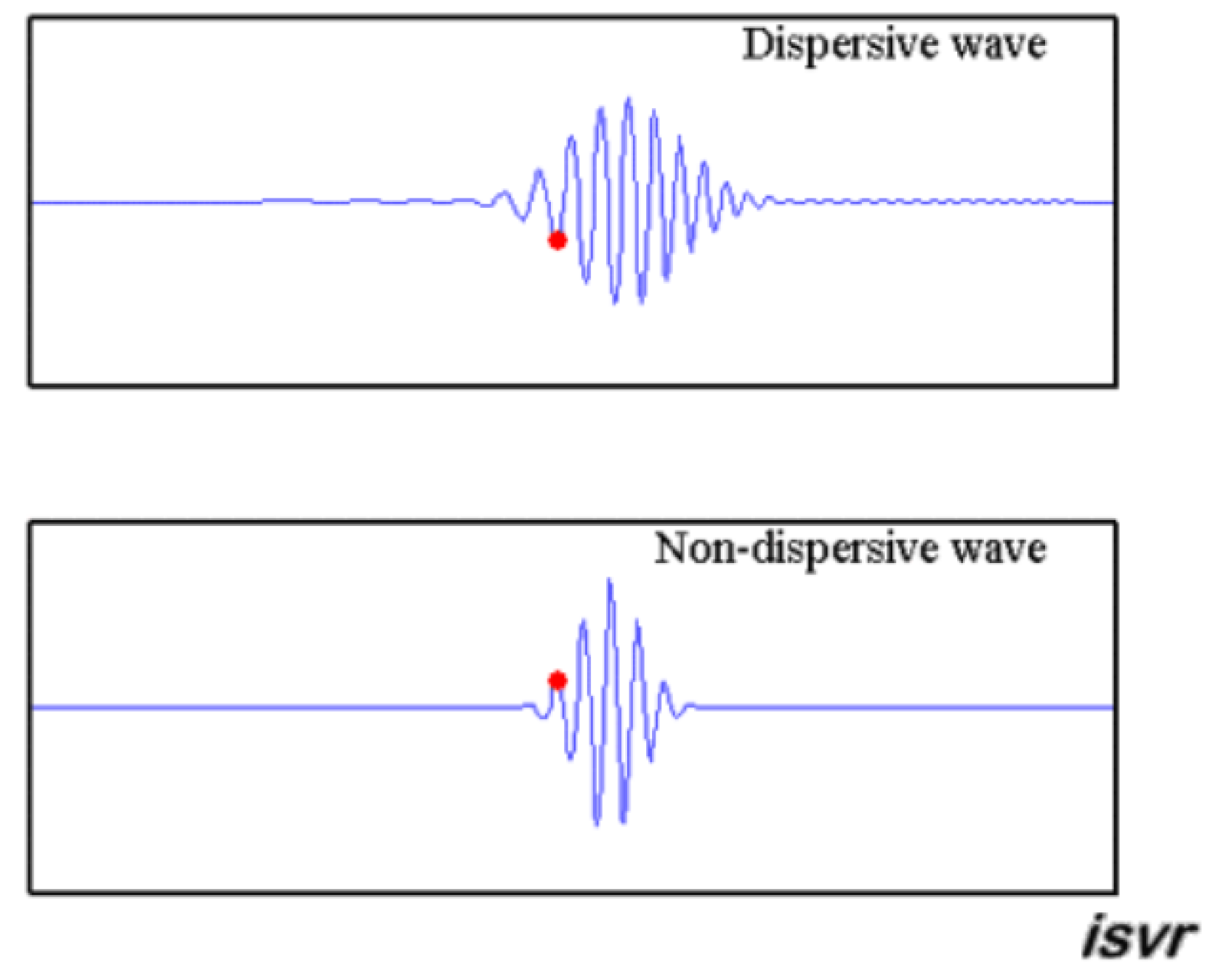
4.6. Dispersive and Nondispersive Groups: A Comparison with a Dispersive Substrate
Dispersive mechanisms are best displayed using animations, and good examples are available online from ISVR [
23], and also on Wikipedia as “phase velocity”. As shown in
Figure 4, these wave packets can propagate without dispersion, but with the packet continuously changing in form as the peaks apparently move through the envelope. The stability of the bell shape was tracked in our models for more than a 500 m range, showing that there was no dispersion within the packet.
The observed structure of the groups or modes generated within the graded sediment substrate could be compared with a dispersive substrate, that of a steel tank base. Transverse (here, “upward”) vibrations within such plates will radiate sound into an adjacent fluid space if the wavelength within the plate is larger than the corresponding wavelength within the fluid. However, if the wave speed within the vibrating solid is less than that of the compression waves within the fluid, an evanescent pressure field is set up in the fluid near the interface.
The steel baseplate of the tank model was made 0.125 m thick to give a suitably slow speed for 16 Hz flexural waves, a frequency commensurate with results for the graded seabed model. The solid motion was predominantly vertical, but the water particle response shown in
Figure 5 had both horizontal and vertical motion.
The underlying dispersion is described by the mathematics of the flexural (bending) waves being driven in the baseplate, as given by Fahy [
21]:
The propagation speed,
cb, for these bending waves is dependent on the frequency,
f, as well as the material properties, including the mass per unit area,
m. The bending stiffness
D is given by the Young’s modulus,
E; the Poisson ratio,
ν; as well as the plate thickness,
h. (Timoshenko et al.) [
24].
The dispersive character could be clearly seen in snapshot views of the impulsive wave train as it propagates.
At 0.35 s, the wave train was well established, seen in
Figure 6 as a snapshot including node 600 at radius 64 m. The acoustic pressures in the water were well correlated with the deformation of the adjacent steel plate.
In
Figure 7, at 0.8 s the pulse has moved out from node 600 to include node 800 at a 192 m radius. The strong dispersion dramatically increased the length of the wave train. This view had a reduced magnification, with the extended wave train almost extended to the edge of the FE model at a 256 m radius. Note the lack of significant reverberation at this time.
4.7. A Comparison of Different Modes in the Graded Model
The bell envelope shown in
Figure 3 occurred again (
Figure 8), showing two separate bell-shaped modal envelopes in water. The variation with time of the water particle velocity components were plotted, as was the vector magnitude, the particle speed.
The early mode data in
Figure 8 was selected (1.5 s to 1.95 s) and plotted as a hodograph below the time series. This shows the locus of the motion of the water particle as the early mode passed. A second hodograph shows the data for the period 1.95 to 2.35 s, after a brief moment of inactivity.
This hodograph data display was so named by W.R. Hamilton [
25], and provided additional insight into the motion. Unlike the solid motion, the water particles followed a nearly circular path. As more cycles were included within the envelope, more circuits were observed. For a continuous wave, a single circle would be followed repeatedly, but for an impulse, the motion had to start and stop at the origin.
The arrows show the direction of circulation, which is described as retrograde, with the horizontal velocity being at a maximum in the direction of the source at the moment the upward displacement was at a maximum.
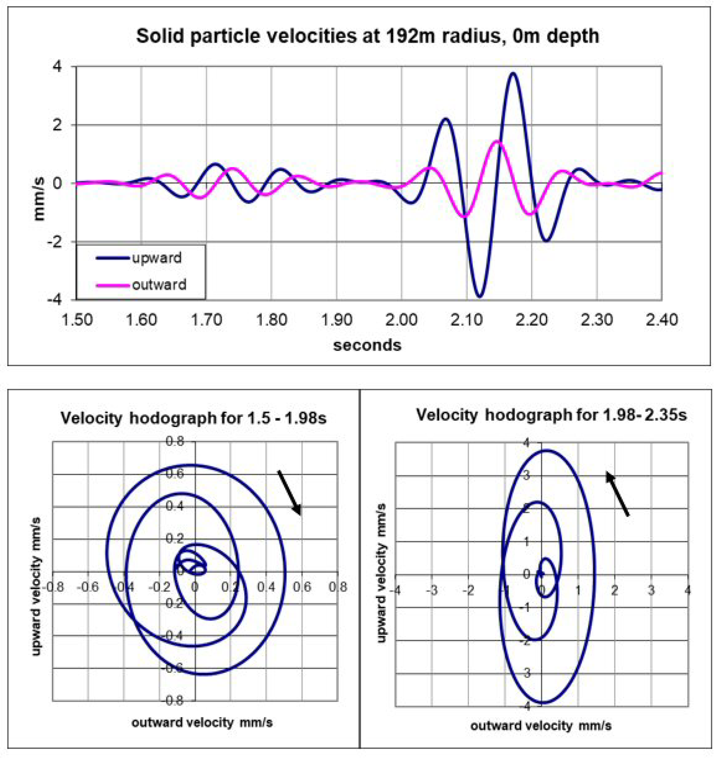
In
Figure 9, the motion of a solid particle at the interface is shown. Now the hodographs are highly contrasting both in shape and direction. The less-intense early mode travelled faster (~140 m/s) than the more intense mode, which was slower (~117 m/s).
The more intense retrograde mode is that which we previously studied, but we intended to further investigate the prograde mode, which cannot exist in the Rayleigh half-space model, but propagates stably in the graded half-space.
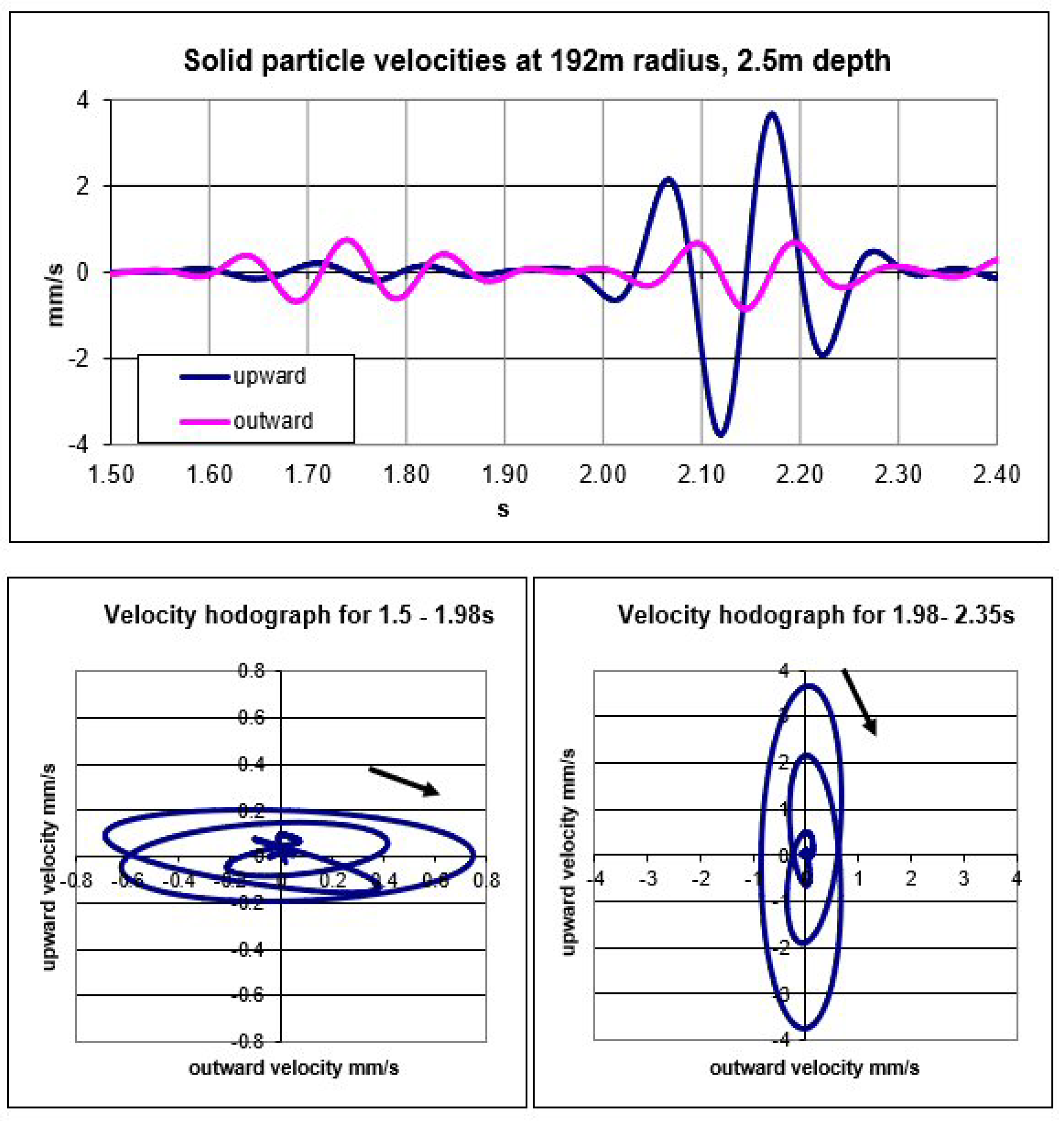
In
Figure 10, both hodographs are prograde, but with contrasting shapes. These examples show how the graded model dispersed energy between modes, but we found no evidence of dispersion within individual modes. In 2018, we showed this by tracking their peak intensities against travel time. There was a good fit for the cylindrical spreading of peak energy, as the wave circumference increased without dispersion.
For the later mode, a change in direction of the solid motion occurred at a critical depth (~1.1 m) below the interface. Here, there was no horizontal motion. This phenomenon was described by Rayleigh for the interface waves in a solid half-space, and this similarity showed how the later mode in the graded seabed model was a version of the “Rayleigh wave”. The existence of prograde waves at depth was thus expected, but the Rayleigh theory only predicted retrograde motions at the surface with no dispersion.
In contrast, the energy in the graded model was dispersed into at least two modes that travelled at different speeds, and thus reduced the intensity to be found at a distance, but this dispersion was still much less than that to be expected over a layered seabed.
4.8. The Contrasting Group and Phase Velocities
Time profiles at two positions were used to measure the travel speed. The Gaussian envelope bell form helped by allowing a precise fit to the data extracted from the FE analysis. This speed was found to be 117 m/s when the material shear speed, V
s(0), at the interface was specified as 128 m/s. This ratio of 91.4% can be compared with the interface wave speed for the Rayleigh model given by Achenbach [
15] as varying from 86.7% to 95.5% dependent on the Poisson ratio of the uniform solid in the half-space. We estimated the precision of our measurement at ±0.5 m/s, but recognize the uncertainty of the FE procedure, which depends on the accuracy of many successive calculations.
A mathematical analysis of the impulse clearly would be better, if one could be found to give a closed-form solution. However, a discussion with Godin (private communication) suggested that his published method [
17] for a power-law depth profile cannot cope with the step change at the interface of our model.
4.9. The Influence of the Depth Profile Gradient on the Speed of the Displacement Wave
The gradient of the material shear wave speed with depth has been found to influence the speed of the displacement wave, cd. We know that the greater this depth profile gradient, the more rapidly the wave energies are refracted back to the interface.
Figure 11 shows a snapshot view that was used to measure the wavelength. With a specified frequency of 80 Hz, this determined the displacement (or “phase”) wave speed. The smallest elements in this fine-mesh density model were only 0.0625 m wide.
Five whole waves were selected, and the corresponding number of elements was found to be 119. This gave a wavelength of 1.4875 m and a wave speed of 119 m/s. The gradient in this model was 4 (m/s)/m. FE models in a sequence were run, each with different values of the gradient. The results are shown in
Table 1. They were of limited precision, estimated at ±0.5 m/s, but showed a clear trend.
Improved methods for using the FE methodology to determine cd are being considered, including better postprocessing. The precision was increased by using a finer mesh density, but at the expense of much longer run times and large data files.
Making these changes also helped to show that the results were not an artifact of the modeling process. Other checks on the validity of the FE process include changing the boundary conditions of the FE model. A change from a rigid boundary (no motion) to a soft boundary (no forces) would change the phase of any reflected waves, so that the extent of any such reverberation can be monitored and shown not to affect the conclusions.
4.10. The Evanescent Form of the Associated Pressure Fields in the FE Modelling
Figure 1 shows the distribution of acoustic pressures within the water as the wave passed. A rapid reduction in amplitude is shown by the green coloration well away from the interface. This distribution was typical of an evanescent field. No energy was radiated away from the interface, with the stored energy being supplied by the travelling seismic interface wave, and recovered for onward transmission, assuming there were no losses. In practice, there will be absorption, as the acoustic energy is converted to heat, but that will depend on the local circumstances, and was not modeled here.
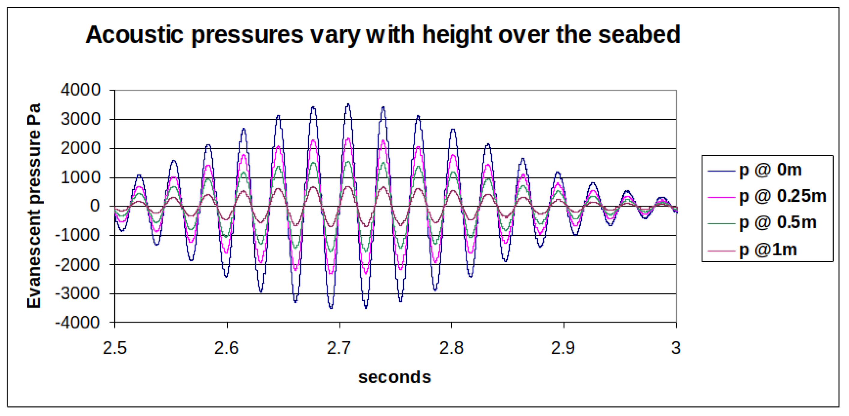
Figure 12 shows the acoustic water pressures as a function of the height above the interface. Notably, the waveforms of these time profiles were all in alignment, with peaks occurring simultaneously.
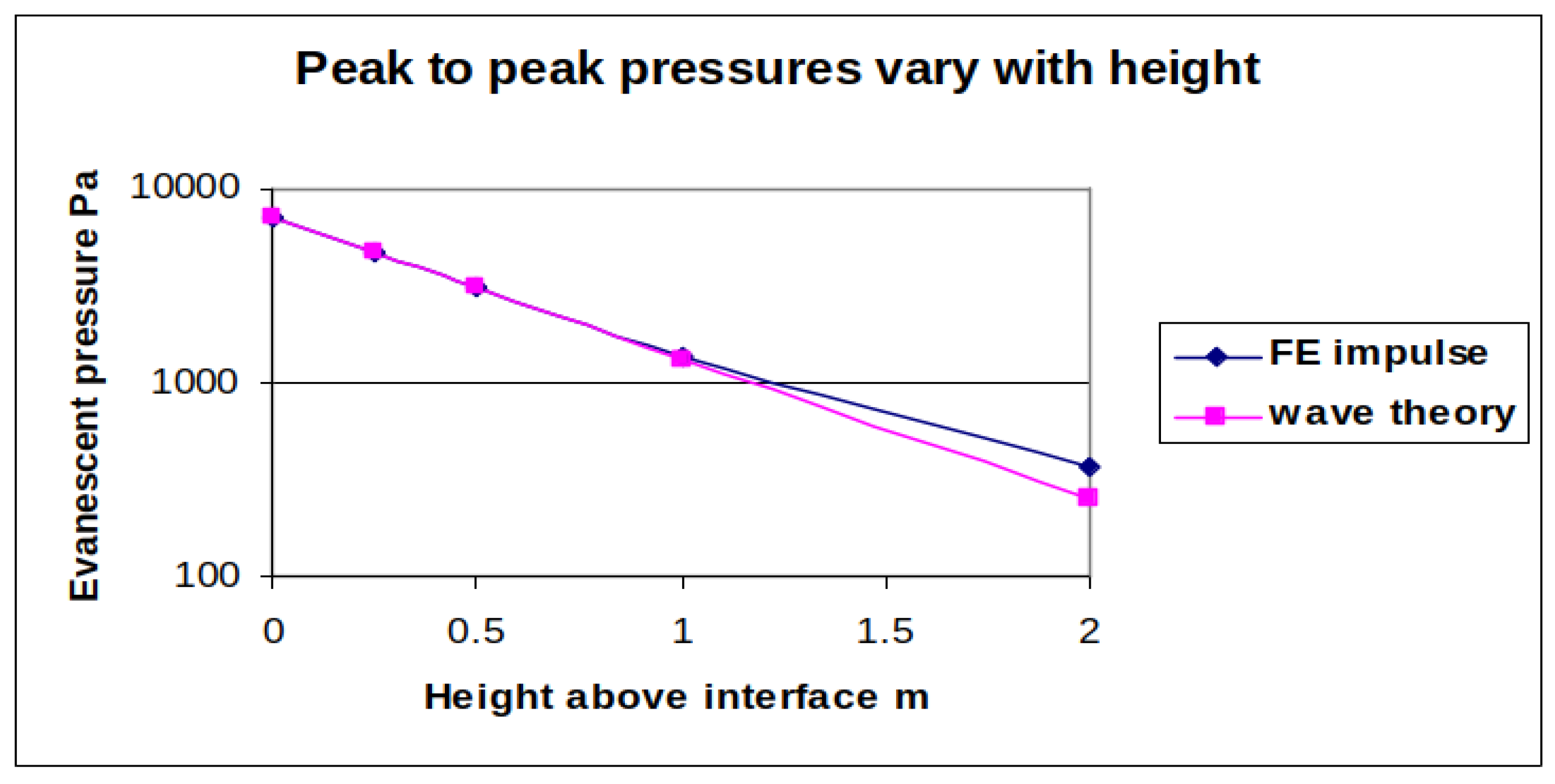
The good fit to the straight line of the continuous wave theory in
Figure 13 shows that the evanescent water field followed an exponential decay within this FE model. The field thickness was 0.6 m for the fitted line, shown for a frequency of 32 Hz. The deviations at greater heights were due to reverberation in the model, but were small compared with the pressure levels at the interface.
The displacements below the interface were also shown to be evanescent, with an eventual exponential decay occurring at depths >10 m, but these fields were more complicated than those in the water above. Different modes travelled at different speeds, with changes in the direction of the motion at defined depths, as can be seen in contrasting
Figure 9 and
Figure 10. However, the simpler evanescent water pressure field was independent of the horizontal motion of the solid.
4.11. Linking the Acoustic Pressure and the Horizontal Water-Particle Velocity
For continuous plane waves in open water, well away from boundaries, the ratio of acoustic pressure to the water particle speed is called the specific acoustic impedance (Kinsler et al. [
22]). This is a scalar, dependent on the water density, ρ
w. Only compression waves are propagated in a fluid, and the particle motion lies along the direction of energy propagation, so that the speed is just this velocity component. However, in an evanescent field, the water particles move with velocities that have components in multiple directions.
It is then appropriate to use the inverse of the impedance, the admittance, as a complex vector, which is the water-particle velocity vector, u, divided by the scalar pressure,
p. The complex vertical admittance component is imaginary, the pressure waveform is out of phase with the vertical velocity, and there is then no work done on the fluid by the motion of the solid (Fahy [
21]). We denoted the vertical velocity component as u
v and the horizontal component as
uh.
Then, the vertical admittance becomes:
The horizontal admittance is a real quantity and derived in the same way as that for continuous plane waves (Kinsler et al. [
22]), but is dependent on the displacement wave speed,
cd.
The square root term in Equations (3) and (8) can now be considered as a “shape factor”, since it will control the shape of the water-particle hodographs. When cw >> cd, this factor is close to unity, and the hodograph is circular, but as the ratio decreases, the hodograph becomes elliptical with comparatively reduced vertical motion.
4.12. A Comparison of Water-Particle Motions in the Evanescent Field to Those in Plane Waves
With the knowledge that it is the water-particle motion that is sensed by many subsea creatures, it is common to infer this parameter from a measured acoustic pressure, using the specific acoustic impedance, ρwcw. However, this inference is invalid when the acoustic pressure is created by a seismic interface wave and the displacement wave speed, cd, should be used in place of cw.
It is convenient to use a unitless velocity-to-pressure ratio (VPR). This is done by comparing the evanescent field horizontal admittance to the value for acoustic plane waves in open water. From the data shown in
Figure 3, we found a VPR just over 12.0 for the windowed wave packet used.
In contrast, if we used Equation (9) for a continuous wave, with the value for c
d of 119 m/s for a value of gr = 4 (
Table 1) and a value of
cw = 1500 m/s, we calculated a VPR of 12.6. More work is planned to investigate how this difference was influenced by other factors, such as the properties of different finite-length wave packets. However, it was clear that the VPR was substantial in all realistic cases, and a value of 12 provided a fair working estimate. This showed how much more significant the water-particle motions were in comparison to the acoustic pressures in the evanescent field.
It is also interesting to measure this ratio in practice by comparing the values from a hydrophone with a water-particle velocity sensor.
5. Additional Field Trials
5.1. Methods
The prediction of the strong linkage between the local evanescent pressures and the horizontal water particle velocity led to a trial in the still waters of Wraysbury reservoir, where a test facility is operated by the National Physical Laboratory (NPL) Teddington, London.
Figure 14 shows the stainless-steel sledge fitted with various instruments on cables to allow their deployment onto the clay bed 20 m below the raft. The central housing contained a set of three orthogonally mounted geophones. This is the same instrument that was deployed into the Rhine estuary at Kinderdijk and reported by Hazelwood and Macey 2016 [
18]. As before, the deployment used an extra line attached to the sledge prow (
Figure 14) to tow the sledge a short distance, thus aligning it with respect to the raft.
Two additional instruments were added, each with their own cables. A hydrophone was supplied by NPL, and an experimental glass buoy was held in a holster, which allowed it to float clear once deployed into the water. This was then held down by a light coiled spring, which had been previously tested to give a vertical resonance with a low natural frequency <5 Hz.
One of the set of geophones in the buoy can be seen through the glass. The use of more geophones allowed the same low-noise, low-impedance preamplifiers to be used as developed for the Kinderdijk trial. These geophones were well adapted to sense velocity over the frequency range 10–200 Hz, with a flat sensitivity of 20 V/(m/s). It was thus useful to compare their outputs with that of the hydrophone, which had a pressure sensitivity that was flat over the same frequency range.
The seismic interface wave was generated by the impact of a 20 kg bronze cylinder with the bed of the reservoir, after being dropped from the raft. The cylinder was streamlined with a cylindrical rear fin to maintain its attitude during the descent, and recovered by winch using a rope, flaked out on the raft deck before the drop to minimize drag. Several drops were made with similar results.
5.2. Results
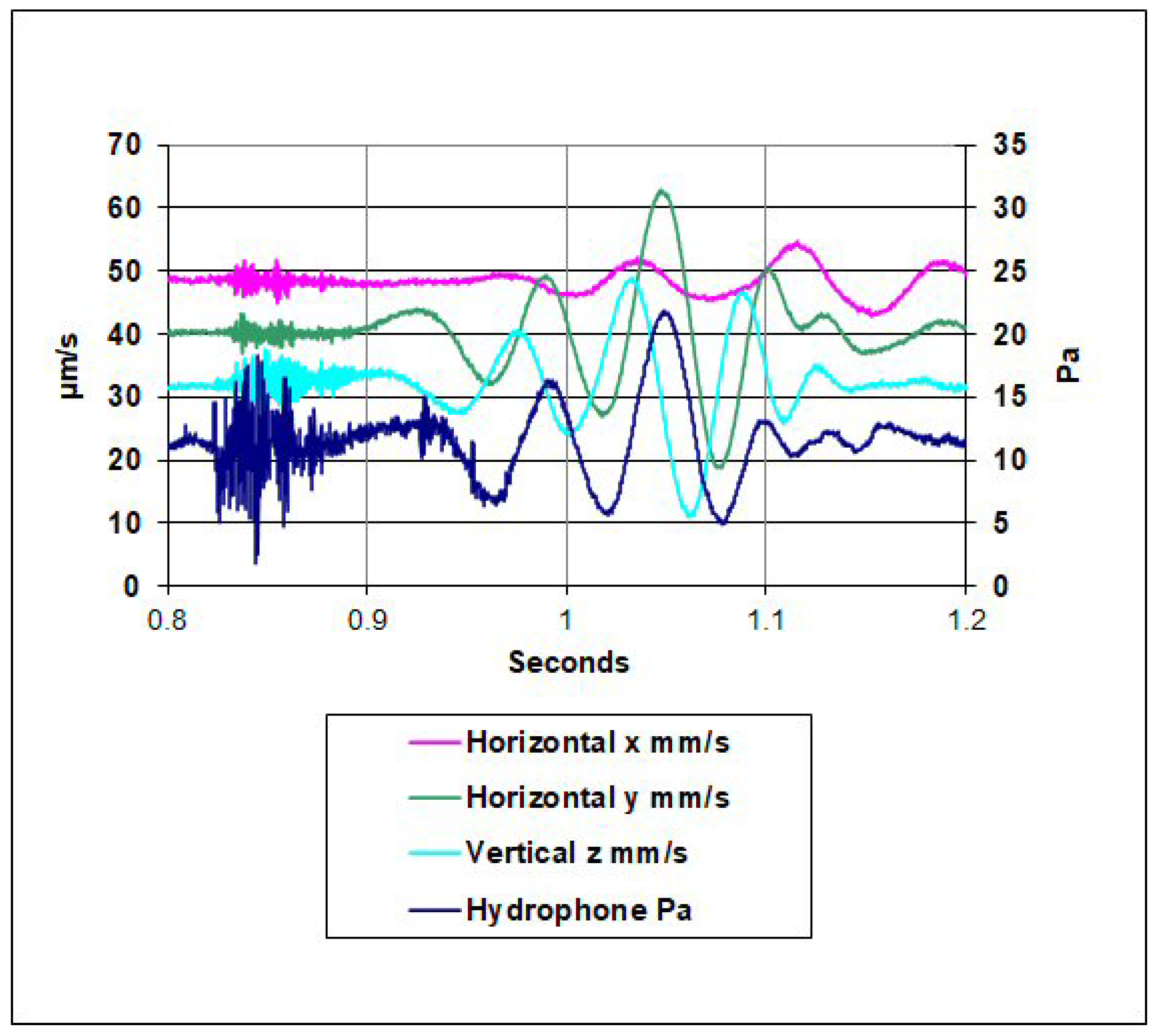
The principal finding shown in
Figure 15 was that the shape and phase of the hydrophone time series (dark blue) largely matched that of the horizontal y velocity component (green) given by one of the geophones. The data shown was used to estimate the VPR. The peak-to-peak (p-p) amplitude of the y component data was 43.6 μm/s. The amplitude of hydrophone data was 16.5 Pa. The ratio of pressure to velocity was 378 Pa/(mm/s).
Comparing this with a typical open water impedance of 1500 Pa/(mm/s) gave a VPR of 4.0, much less than the continuous wave theoretical value of 12.6 or the FE model VPR of 12.0. This was disappointing, and suggested the need to further investigate the performance of the experimental glass geophone buoy. We also recognized the risk that the heavy sledge may have affected the nearby water motion, and that we did not have details of the properties of the sediment. However, the confirmation of the wave-packet shape was encouraging.
6. Conclusions
The change of the forcing impulse in the FE model provided more results for higher frequencies than the previous papers. The Gaussian windowed cosine form allowed comparisons with analytic mathematical theory for continuous waves, showing similar effects, but with some changes in magnitude.
Additional analysis of the water-particle motions generated by the seismic interface waves showed a Gaussian bell-shaped time series for the water-particle kinetic energies in various modes. This was used in a fit procedure for the wave envelope to allow more precise timing to give better data for the envelope speed.
The displacement wave speed was shown to be controlled by the rate of increase with depth of the material shear wave speed. It was faster than the wave envelope speed, creating apparent movement of the displacement wave peaks through the envelope window. This explained the morphing effect reported for the pulses seen in earlier work.
The retention of energy within the most intense mode, as reported before, was confirmed by the contrast in the dispersion between the modes in the graded model, as well as that for modes generated by a layered model. Other modes were seen to have a quite different structure in the solid, without a change from retrograde to prograde predicted by Rayleigh [
11] for the uniform half-space.
Evanescent pressure fields in the water have been analysed both by flexural plate theory and by the use of FE models, both for the graded seabed and a single-layer substrate. The water-particle motions were shown to be large by comparison to the acoustic pressures, with a large velocity pressure ratio when comparing this effect to that found in open water.
The study has also raised many questions that it is hoped can be answered by future work. More measurements and theory could help further explain the features outlined here.


