Abstract
Breaking waves generated by wave shoaling in coastal areas have a close relationship with various physical phenomena in coastal regions. Therefore, it is crucial to accurately predict breaker indexes such as breaking wave height and breaking depth when designing coastal structures. Many studies on wave breaking have been carried out, and many experimental data have been documented. Representative studies on wave breaking provide many empirical formulas for the prediction of breaking index, mainly through hydraulic model experiments. However, the existing empirical formulas for breaking index determine the coefficients of the assumed equation through statistical analysis of data under the assumption of a specific equation. This study presents an alternative method to estimate breaker index using representative linear-based supervised machine learning algorithms that show high predictive performance in various research fields related to regression or classification problems. Based on the used machine learning methods, a new simple linear equation for the prediction of breaker index is presented. The newly proposed breaker index formula showed similar predictive performance compared to the existing empirical formula, although it was a simple linear equation.
1. Introduction
The wave speed of the wave propagating from the deep sea to the coast decreases owing to the influence of the water depth, resulting in an increase in the wave height and a decrease in the wavelength. Wave breaking begins when the increased wave height on the coast reaches a certain limit of wave steepness. This wave breaking phenomenon is caused by various wave transformations such as shoaling, wave refraction and wave reflection, and is very important in coastal engineering because it induces high external forces such as wave impact pressure on coastal structures, acting as a major external force of cross-shore sediment transport while simultaneously facilitating longshore current in the breaker zone. Particularly, although wave breaking height and depth are crucial design elements of coastal structures, wave breaking occurrence on the seabed slope is difficult to completely explain in terms of theory due to the complexity of its generating mechanism; it is one of the crucial challenges in coastal engineering as research on wave breaking has continued for the past 140 years since the research conducted by [1]. With the development of measuring equipment, hydraulic model experiments on wave breaking have been conducted earnestly since the 1950s. Based on the experimental results, various empirical formulas have been proposed for the quantitative evaluation of wave breaking. In recent years, as the performance of computing power has improved dramatically, studies attempting direct numerical analysis on the mechanism for wave breaking based on computational fluid dynamics (CFD) are rapidly increasing—e.g., [2,3,4,5,6,7,8]. Numerical simulation using CFD has the advantage of considering the influence of viscosity, generation of turbulence, movement of gas, and change in density at the water surface boundary, closely associated with wave breaking. Although numerical simulation using CFD requires a computational cost, it can be a good alternative tool to provide a detailed wave breaking mechanism. Furthermore, using the numerical results can also be synthesized to get fast and reliable estimation of the wave breaking index.
Recently, Liu et al. [9] classified the previously proposed empirical formulae for breaking indicators into four types: McCowan, Miche, Goda, and Munk-type [10,11,12,13], and compared and analyzed each empirical formula with the existing experimental data. Consequently, the Goda-type empirical formula using deep-water wave steepness as a parameter exhibited relatively high predictive performance; however, there was an error due to the beach slope. Liu et al. [9] proposed an empirical formula using the wave velocity of linear theory in shallow water conditions for calculating independent wave breaking index on the beach slope. Kamphuis [14] suggested including both the parameters of beach slope and relative breaker depth in the breaker index formula by comparing the correlation coefficients for the existing formulas. Rattanapitikon and Shibayama [15] proposed an empirical formula that computes the breaking wave height and wave breaking depth explicitly. Goda [16] presented a revision of his empirical formula [12] to complement the low wave breaking predictive performance on the steep slope of the existing empirical formula. In addition, Xie et al. [17] proposed a semi-empirical formula verified by inducing an analytical solution from the shallow water equation and applying existing experimental data to accurately predict the wave breaking depth. However, since most empirical formulas include the breaking wave height and the breaker depth simultaneously as a function of other variables related to breaking phenomena, either the height of wave breaking is required to predict the breaker depth or vice versa; namely, it is not easy to compute the breaker index explicitly. For a fast and reliable estimation of wave breaker index without the aid of numerical methods, the breaker height formulas are commonly used together with the linear wave shoaling which is most widely used in practice, or a schematic plot of the formula. Therefore, although a number of the existing breaking wave formulas, statistically determined from the laboratory data, have been proposed for more than one century, they might cause specific errors in engineering applications in the use of the linear wave shoaling and schematic approaches. On the other hand, if the breaking wave height and the breaker depth can be predicted only with limited information such as deep-water wave steepness and beach slope, which are relatively easier to obtain, it can be instrumental in various coastal engineering problems.
Conversely, machine learning (ML) algorithm, a field of artificial intelligence in which a computer can automatically produce certain rules by retrieving statistical structures from input and output data without being explicitly programmed by the user, is being actively used in various fields. The first attempts of real ML began 60 years ago with the work of Samuel [18] that programmed a computer to play chess. Recently, along with the advent of big data owing to the reduction of data storage costs, the development of various ML algorithms, and the advancement of computing technology, research involving ML has been actively conducted in various fields. In the field of coastal engineering, the number of studies using ML including is steadily increasing to solve various engineering problems. Kim and Park [19] proposed a design and reliability analysis model of a rubble mound breakwater based on the ML algorithm. Kazeminezhad and Etemad-Shahidi [20] and Etemad-Shahidi et al. [21] applied the ML algorithm to calculate the run-up height of a vertical pile and the quantity of overtopping for a vertical structure. Formentin and Zanuttigh [22] proposed a new formula based on the ML algorithm to predict the effect of decreasing the crown height on the quantity of overtopping. James et al. [23] built an ML-based model for wave estimation on the coast and showed that the computational cost was dramatically reduced compared to the existing SWAN model. Stringari et al. [24] and Buscombe et al. [25] proved that effective wave tracking in the surf zone is possible using the ML algorithm. Alqushaibi et al. [26] found that the enhanced weight-optimized ML models based on the sine cosine algorithm (SCA) have the capability of improving wave prediction. However, most of them are limited to artificial neural networks (ANNs). ANN is an ML model that is widely used in various fields owing to its feature that it is an engineering modeled learning algorithm similar to a neural network in a living system that can handle nonlinearities. However, it is reported that the predictive performance of ANN largely depends on the quality and size of training data for learning and that the experience of the developer through trial and error is required to establish an optimal network [27,28]. Additionally, it is still difficult for ANN to identify the optimal parameter in the learning process, and it lacks the function to explain the process between the input and output variables. These shortcomings of ANN may hinder many engineers from easily accepting ANN models. In addition, most previously proposed empirical formulae for wave breaking prediction are based on exponential or hyperbolic functions, making it difficult to calculate.
This study aims to propose a new simple equation for wave breaking prediction using a supervised learning ML algorithm based on a linear regression model that can explain the relationship between the input and output variables related to breaking. The hydraulic model experimental data obtained from the existing breaking studies conducted on a certain slope were used as the training data and evaluation data for ML. The ML algorithm is a basic linear model (LM) and a support vector machine (SVM), which is frequently used for good predictive performance in research related to regression problems. Using the selected ML technique, a model for predicting the breaker index occurring on the slope owing to shoaling is constructed, and its applicability is presented through comparison and analysis with the previously proposed empirical formula. In addition, this study proposes a new equation for the breaker index that can be easily calculated explicitly and applied to various problems related to wave breaking.
2. Experimental Data Related to Wave Breaking
2.1. Definition of Physical Quantities for Wave Breaking
As described above, hydraulic model experiments on wave breaking have been steadily conducted by many researchers, thereby accumulating considerable experimental data. However, the definition of the wave breaking point does not accurately match each experiment. There are some cases where wave breaking is defined as the point at which the wave height reaches the maximum, the point at which the front of the wave becomes vertical, or the point at which the horizontal component of the water particle velocity at the wave crest exceeds the wave velocity. Besides these definitions of breaking point, the various possible definitions in which radiation stress, water particle acceleration and the Bernoulli equation are used can be listed by Singamsetti and Wind [29]. Therefore, depending on the definition of the wave breaking point, the breaking wave height may be slightly different for each experimental data. Furthermore, to define the wave breaking point might be rather subjective in which judgment is always involved via the experimental process. The wave breaking depth may also differ depending on whether the still water level or the mean water level is applied. Unfortunately, not all authors explain the definition for judging the breaking height.
Because a large part of the data on the results of existing laboratory model experiments in this study was obtained from the previous studies by [17,30,31,32,33,34,35,36], incipient wave breaking was defined as the point of time when the front of the wave becomes vertical as defined by [30,31,34,35,36] although there is a more complex issue in defining the wave breaking point. The still water level was also applied to the wave breaking depth without considering the role of hydrodynamics such as wave setdown and setup. Figure 1 shows the definition of the physical quantities for the wave breaking. As shown in the figure, the breaking wave height is the vertical distance from the wave crest to the wave trough, and the wave breaking depth is the vertical distance from the bottom to the still water level considering the beach slope .
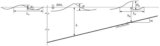
Figure 1.
Definition sketch of wave at incipient breaking.
2.2. Collection of Experimental Data
Existing experimental data for wave breaking were obtained by referring to the studies of [17,30,31,32,33,34,35,36]. Table 1 lists the conditions and range of experimental data used in this study. A total of 858 experimental data were obtained from previous studies, and the beach slope ranged from 0.01 to 0.2. However, the experimental data of Xie et al. [17] and Lara et al. [33] did not provide information on the breaking depth and on each breaking wave height, respectively; the data of each experiment were limited to predicting the breaking wave height and wave breaking depth. It is noted that the collected data listed in Table 1 are monochromatic wave breaking carried out in the wave flume.

Table 1.
Summary of historical experimental data set on breaking waves.
2.3. Dimensional Analysis and Setting Target Variables for Wave Breaking Index
It is well known that wave breaking in shallow water has relationships among the breaking wave height, the local water depth, wavelength, bottom slope, and other potential parameters [9]. To find the target variable, we assume the wave breaking has a potential correlation among deep-water wavelength , offshore wave height , and bottom slope . For the dimensional analysis, the characteristic length parameter can be introduced to represent the breaking characteristics such as the breaking height and the water depth . The functional relationship between the independent variables , , , and water density can be expressed as follows:
In the dimension analysis, the bottom slope is not included because it is a dimensionless quantity. The Buckingham Pi theorem [37] was applied to Equation (1) and out of this analysis two dimensionless quantities, and , were formed as follows:
The functional relationship between the two quantities can be expressed as:
where the characteristic length scale related to the wave breaking can be taken by the breaking height and the water depth . In addition, new dimensionless terms, and , can be obtained by combining and . Therefore, based on the result of the dimension analysis, we can describe the wave breaking by using the relationships between dimensionless possible variables such as the ratio between the breaking wave height and wave breaking depth (McCowan-type), the ratio between the breaking wave height and wavelength at the wave breaking point (Miche-type), the ratio between the breaking wave height and deep-water wave height (Munk-type), and the ratio between the breaking wave height and deep-water wavelength (Goda-type).
Figure 2a,b correspond to the wave breaking indices of McCowan-type and Munk-type, respectively; accordingly, empirical formulae for many wave breaking predictions have been proposed [9]. In addition, Pearson’s correlation coefficient (PCC) between the deep-water wave steepness , the beach slope , and the nondimensionalized breaking wave index are also presented as the table in the figure. Pearson’s correlation coefficient represents a linear correlation between each variable. In general, when the absolute value of the correlation coefficient is 0.3–0.7, it is interpreted as a clear linear relationship, and when it is above 0.7, it is interpreted as a strong linear relationship. Figure 2 shows that the ratio between the breaking wave height and the wave breaking depth and the ratio between the breaking wave height and the deep-water wave height has a clear negative linear relationship with the deep-water wave steepness , and they also have a strong linear relationship with the beach slope . However, the wave breaking height index applied in Figure 2 has a correlation coefficient of 0.7 or less and does not have strong linearity; therefore, it cannot be used as a suitable target variable for wave breaking prediction using linear regression.
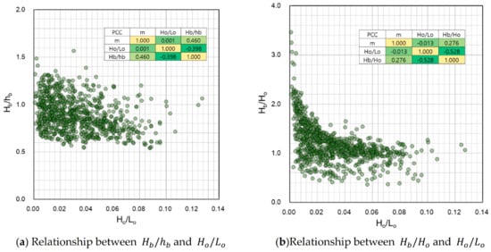
Figure 2.
Relationship between breaker indices: (a) , (b) and deep-water wave steepness by historical laboratory experiments.
Similar to Figure 2 and Figure 3 is a schematic result of a Goda-type breaking wave height index that is nondimensionalized to the breaking wave height as a function of . As for the wave breaking depth, the wave breaking height index nondimensionalized to the wavelength is applied. As shown in Figure 3, and have a correlation coefficient higher than 0.9 to , indicating a strong linear relationship.
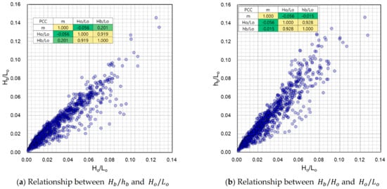
Figure 3.
Relationship between breaker indices: (a) , (b) and deep-water wave steepness by historical laboratory experiments.
One of the goals of the study is to propose a new linear equation for predicting wave breaking indices; therefore, Equation (4) with high linearity was set as the target variable for the final prediction of ML.
Here, and , which are the target variables of ML, denote the breaking wave height index and wave breaking depth index, respectively. The target variables are a function of the beach slope and deep-water wave steepness .
3. Characteristics of Existing Empirical Formulas for Wave Breaking Prediction
The existing theoretical or empirical formulas proposed for wave breaking are based on linear wave theory or results of hydraulic model experiments performed for impermeable slopes or beaches consisting of sand. Since Miche [11] proposed Equation (5), which states that waves start breaking when the particle velocity exceeds the wave velocity at the crest of traveling-wave, various hydraulic model experiments have been conducted for wave breaking.
Using the accumulated experimental data, many researchers have proposed empirical formulas to predict the wave breaker index. Because the equation proposed by [11] is based on the maximum deep-water wave steepness (), the wave breaking height is overestimated, and the beach slope is not considered. Le Mehaute and Koh [38] were the first to propose the empirical formula of Equation (6) for wave breaking height, which simultaneously considers deep-water wave steepness and beach slope.
This equation has been modified by many researchers. As a representative example, Ostendorf and Madsen [39] proposed the following empirical formula by modifying the Equation (6) to consider the wave breaking height according to the beach slope.
Kamphuis [14,40] carried out the hydraulic model tests for regular and irregular waves on natural beach conditions and found that the wave breaking height can be calculated by Equation (8), incorporating the local wavelength, breaking wave depth and the beach slope.
Rattanapitikon and Shibayama [15] have proposed Equation (9) for wave breaking height and depth using deep-water wave steepness, based on available experimental data.
Goda [16] modified his previous wave breaking equation [12], which is expressed as a function of deep-water wave steepness, to improve the prediction performance of steep beach slope, and proposed Equation (10), which uses the ratio of breaking depth to deep-water wavelength as a parameter.
where is a constant, which is 0.17 and 0.12 for regular and irregular waves, respectively. In contrast, Liu et al. [9] proposed the following empirical formula using the wave velocity of small amplitude wave theory under the shallow sea condition to estimate the independent wave breaker index on beach slopes.
where , is the wavelength at the wave breaking point,, is the gravitational acceleration, and is the wave velocity at the wave breaking, which is defined as follows:
However, the equation proposed by Liu et al. [9] is difficult to use in practice because iterative calculations are required to derive . Recently, Xie et al. [17] proposed the semi-empirical formula of Equation (13) to estimate the breaking depth of plunging breaker type.
Figure 4 shows the results of predicting the dimensionless wave breaking height by applying the empirical formulas proposed by Rattanapitikon and Shibayama [15] and Goda [16] described above. The dotted lines in the figure indicate the error range of 20%. The prediction results of wave breaking height in Figure 4a show that the proposed formula of Rattanapitikon and Shibayama [15] for the dimensionless wave breaking height overestimates the experimental results for relatively gentle beach slopes, but underestimates for relatively steep beach slopes. In contrast, the results from Goda’s formula [16] in Figure 4b demonstrate that the dimensionless wave breaking height is overestimated for relatively steep beach slopes . The average error rate of the dimensionless wave breaking height prediction by the empirical formulas of Rattanapitikon and Shibayama [15] and Goda [16] was 21.5% and 13.3%, respectively. However, because the experimental results of [27,33] in Table 1 did not provide the relationship between the wave breaking height and breaking depth, they were not used for the prediction of wave breaking height by the Goda’s empirical formula [16] shown in Figure 4b.
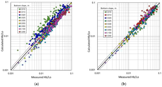
Figure 4.
Comparison of wave breaking height formulas with experimental data: (a) Rattanapitikon and Shibayama (2006); (b) Goda (2010).
Figure 5 shows the results of predicting experimental data of the dimensionless wave breaking depth by applying the empirical formulas of Rattanapitikon and Shibayama [15] and Xie et al. [17]. The prediction results of the dimensionless breaking depth show that the accuracy decreased compared to the prediction results of wave breaking height. In particular, the empirical formulas of Rattanapitikon and Shibayama [15] and Xie et al. [17] for breaking depth overestimate the dimensionless breaking depth , and the average error rates against the experimental results are 31.4% and 29.8%, respectively, which are high values. The scatter index (SI) [41] and the coefficient of determination (R2) [42] were applied as measures for a more quantitative evaluation on the degree of prediction for the existing empirical formulas of wave breaking height and breaking depth. As shown in Equation (14), SI is a dimensionless error metric obtained by dividing the root-mean-square error by the mean of experimental data, whereas R2 in Equation (15) indicates the degree of fit for the estimations of the prediction model expressing the experimental results.
where refers to experimental data, refers to the predicted value, and refer to the mean of experimental results and predicted values, respectively, and n is the number of data. The smaller the SI and the higher the R2, the better the correspondence between experimental and predicted values.
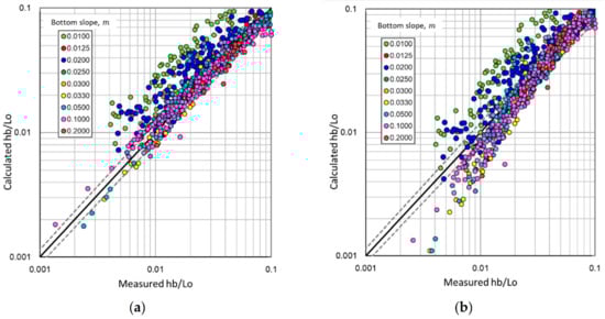
Figure 5.
Comparison of wave breaking depth formulas with experimental data: (a) Rattanapitikon and Shibayama (2006); (b) Xie et al. (2019).
Table 2 shows the degree of prediction for the existing representative empirical formulas of wave breaker index discussed in Figure 4 and Figure 5. According to Table 2, the existing empirical formulas provide a better prediction performance for wave breaking height than for breaking depth. Furthermore, in the scope of wave breaking experimental data applied in this study, Goda’s formula [16] shows better prediction performance for wave breaking height, whereas the Rattanapitikon and Shibayama’s formula [15] shows better prediction performance for breaking depth.
Table 2.
Results of error analysis.
4. Wave Breaking Index Prediction Model Using Machine Learning
ML refers to analyzing and learning given data using a certain learning algorithm and classifying new data or predicting values based on the learned data. In other words, learning is a crucial process in ML as it improves predictive performance for new data through learning based on data and experience. Thus, the learning methods of ML can be divided into supervised learning and unsupervised learning. Supervised learning is a method of training models using data with correct answers and is used to solve most classification and regression problems. Conversely, unsupervised learning is a method of grasping the relationship in the main composition (characteristic) of data; clustering is a representative example. In addition, reinforcement learning learns to maximize the reward in the current state under the rules involving rewards and punishments and is known to be widely used in game programming. In this study, supervised learning ML was applied as it aimed to predict the wave breaking indices based on experimental data on wave breaking. The ML technique applied in this study is briefly described as follows.
4.1. Linear Model
Linear regression model (LR) is a straightforward algorithm that can easily implement to give satisfactory results, particularly in supervised learning. In addition, the ML models using LR can be trained easily and efficiently even on relatively low computational power systems due to their considerably lower complexity compared to other complex algorithms. However, since LR basically assumes a linear relationship between the input and output variables, it also has the disadvantage of not being able to properly fit a complex data set. This drawback of LR can overcome by constructing polynomial features that can be extended by LR.
As described in Section 2.3, we also found that the dimensionless wave breaking height and breaking depth have strong linear relationships with deep-water wave steepness , respectively. Furthermore, the main object of this study is to propose an alternative wave-breaking formula that can be easily estimated and used in practical engineering applications with a simple form. For this reason, LR is chosen to predict wave breaking.
LR is one of the simplest ML algorithms that assumes the linearity of Equation (16) for the output value with respect to the input value, considering the feature variable (input value) affecting the target variable (output value) .
where denotes the constant term, and denotes the regression coefficient vector of the feature variable.
When the hypothesis to predict the output value for the input value, is defined as , the ML should perform learning to minimize the difference between the hypothetical output and actual output . In ML, the loss function enables learning with a minimized difference.
where denotes the total number of data, and the superscript denotes the data element. As shown in the above equation, in a general LR, learning is performed to minimize the mean squared error (MSE) of the actual output and predicted output. Therefore, overfitting may occur in the training data applied to learning, resulting in a degradation of predictive performance with a new data set. To prevent this, a regularized LR that improves overfitting by controlling the size of the regression coefficient is used. Regularized LR includes ridge regression (RR) by applying L2-norm, lasso regression (LAR) by applying L1-norm, lasso regression by applying L2-norm, and elastic net (EN) by applying L1-norm and L2-norm simultaneously, according to the shrinkage penalty function applied to the cost function. In this study, the RR derived in Equation (18), which uses L2-norm for the regression coefficient as the penalty function, was applied as the regulated LR.
where is the hyperparameter that requires empirical adjustment by the user.
Conversely, as the cost functions, such as LR, RR, LAR, and EN, use MSE, the loss function owing to the outliers that are exceptional data increases significantly. However, the mean absolute error (MAE) has a relatively small effect on outliers compared to MSE. For the Huber loss proposed by [43], MSE and MAE are applied simultaneously based on a certain range , as shown in Equation (19). In this study, the Huber regression (HR), one of the robust regression methods applying the Huber loss, was used.
In addition, a random sample consensus (RANSAC) algorithm, which is a method of predicting the regression coefficient from the input data with high noise, was applied. RANSAC [44] is a method of extracting an optimal predictive model through iterative learning on a set of randomly extracted data, assuming that outliers exist in the input data. In RANSAC, the number of iterative learning is a hyperparameter, and LR is used as the learning algorithm.
The SVM [45] is a representative model used for classification, regression, and outlier detection. In general linear regression models, MSE is used as the loss function. If there are outliers separated from the normal data distribution, the normal data (inliers) with a low error are affected to reduce the error arising from the outliers, resulting in a degraded predictive performance even with a decreased error. In SVM, a regularization parameter similar to RR is introduced to solve this problem arising from the loss function applying MSE, and concurrently, the following loss function combining L2-norm of the regression coefficient is applied.
where and denote slack variables representing the errors of the data deviating from the margin of error , and denotes a regulatory variable that controls overfitting and generalization. When increases, the possibility of overfitting increases; when decreases, the L2-norm of the regression coefficient is emphasized to perform generalization. The limit of error and regulatory variable are hyperparameters that must be adjusted by the user, similar to Equations (18) and (19). While SVM can be extended nonlinearly through various kernel functions, it was limited to a LR to calculate the regression coefficient for the feature variable in this study.
4.2. Input Variables, Cross Validation and Hyper Parameter Optimization
By applying the deep-water wave steepness and beach slope having a high correlation, with the wave breaking index as the input variables for ML, LM derived in Equation (21) was assumed.
where is the model’s parameter (regression coefficient) vector predicted from ML, containing the bias and the feature weights and , and is the transpose of . Also, is the feature vector, containing and with , and is the matrix multiplication of and . The target variables, and , are denoting the breaking wave height index and wave breaking depth index , which are normalized by deep-water wavelength, respectively. Input variables require a normalization process, such as min–max normalization or z-score normalization, to reflect the same degree of characteristic (distribution) scale for each data. Because the purpose of this study is to calculate the regression coefficient from ML based on a LR, the raw data were applied without normalization.
For the ML model assumed by Equation (21), training should be preceded so that the difference between the hypothetical output and actual data (or ) is minimized, as described in Section 4.1. Training an ML model is setting parameters by finding the value that minimizes the loss functions (Equations (17–20)) of each model so that the model best fits the training data set. As the training data for training the ML model, 60% of the breaking experiment data shown in Table 1 were randomly applied, and the remaining 40% of the test data were used to evaluate the trained model.
However, determining the performance of ML and modifying the parameters using fixed evaluation data may result in overfitting of the evaluation data. To prevent such overfitting in ML, cross validation was applied, which enables the construction of a more generalized model and prevents under-fitting caused by limited data. The methods of cross validation proposed include k-fold, leave-p-out, leave-one-out, and stratified k-fold crossing [46]. In this study, k-fold (k = 5) cross validation, which is the most commonly used method, was applied.
To improve the predictive performance of the ML model, hyper-parameter tuning to control the operation of the ML algorithm is required. The hyperparameter tuning methods include manual search for users to determine the best combination directly, grid search to determine the optimal combination from all combinations of parameters, and random search to determine the optimal combination by random repetitive extraction within the applicable range of hyperparameters [47]. Compared to the random search method, the grid search method provides a more uniform search range with the nine optimization attempts evenly distributed in a two-dimensional space. Conversely, the grid search method only searches three points for an important parameter, but the random search method searches all nine points allowing a more-dense search for an important parameter. In this study, the grid search method involving a simpler search was applied as a linear ML algorithm with a limited number of hyperparameters. Table 3 shows the grid search range for the applied model except for LR without hyperparameter. Figure 6 shows the cross validation and hyperparameter optimization process described earlier.
Table 3.
Grid search range for hyperparameters.
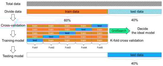
Figure 6.
Process for hyper-parameter optimization using cross-validation.
4.3. Results of Wave Breaking Index Prediction
As described above, in this study, the wave breaking indices were predicted using LR, RR, HR, RANSAC, and SVM, which were the ML algorithms of a linear-based model. To examine the predictive performance of the ML algorithm, the coefficient of determination, indicating the degree of fit for the model to express the target value, was used. The higher the coefficient of determination, the better the correspondence between the target and predicted values.
Table 4 summarizes the results of the regression coefficient and decision coefficient according to the ML algorithm for predicting the wave breaking height index and the wave breaking depth . In Table 4, the regression coefficient corresponds to a bias that can be interpreted as a meaningful interpretation if both and . However, in actual practice, since these conditions are outside the experimental range applied in this study, represents just anchors the regression line in the right place, not a meaningful interpretation. Meanwhile, the first regression coefficient represents the differences in the target variable for each unit difference in bottom slope if the deep-water wave steepness remains constant. Similarly, if remains constant, the second regression coefficient is interpreted as the difference in the target variable for each unit difference in .
Table 4.
Summary of ML training and prediction results for breaker index.
The results of applying the training data and verification data were presented as the coefficients of determination used by the predicted ML model as a measure to predict the target variable. The sensitivity of the coefficient of determination for each ML model differs according to the hyperparameter. The hyperparameters shown in Table 4 represent the optimal results by the grid search method applied to optimize the hyperparameters in this study. Based on the results of the regression coefficients shown in Table 4, the deep-water wave steepness affects the target variable more than the beach slope, and the breaking wave height is more dependent on the deep-water wave steepness than the wave breaking depth.
Figure 7 shows the prediction results for the breaking wave height and wave breaking depth indices for the verification data not used for training using the training results of each ML shown in Table 4. The dotted line in the figure represents an error range of 20%. As shown in the figure, the predicted results of the wave breaking indices by RR are somewhat overpredicting some experimental results. However, overall, it demonstrates a suitable predictive performance with the coefficient of determination as shown in Table 4.
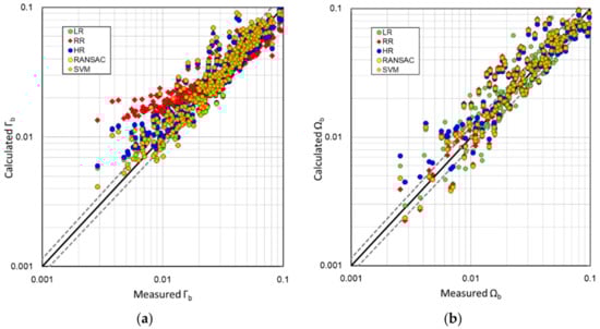
Figure 7.
Comparison of the predicted wave breaking index using test data: (a) estimated wave breaking height; (b) estimated wave breaking depth.
5. Proposal of Linear Formula for Wave Breaking Index
Among the aforementioned linear-based ML algorithms, the regression coefficient of SVM, which showed a satisfactory prediction performance for training and verification data, was used to propose a new formula for easily calculating the wave breaking index. Equation (22) presents the formula for calculating the breaking wave height and wave breaking depth.
The proposed formula for wave breaking index is a linear equation and consists only of a function of the beach slope and deep-water wave steepness, allowing intuitive prediction of wave breaking indices. To verify the proposed formula for the wave breaking index, its predictive performance was compared with that of Equations (9), (10) and (13) proposed by Rattanapitikon and Shibayama [15], Goda [16] and Xie et al. [17], respectively.
Figure 8 shows the calculation results obtained using Equation (22) proposed in this study for calculating the breaking wave height and the water breaking depth. In the figure, the beach slope is divided into three sections to examine the effect of the prediction performance according to the beach slope. The proposed formula for calculating the breaking wave height index shown in Figure 8a has a tendency to overestimate the experimental results in the range of , with a relatively gentle beach slope ; however, it demonstrated satisfactory predictive performance. As shown in Figure 8b, the prediction results for the wave breaking depth show a similar tendency to the prediction results for the breaking wave height; the water breaking depth is overestimated with a gentle beach slope in the range of . Therefore, Equation (19) proposed in this study should be carefully applied in the range of 0.01<< 0.10.
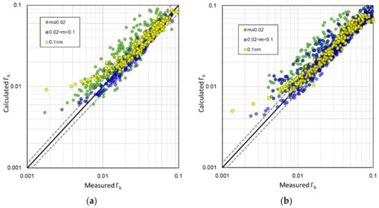
Figure 8.
The predicted results by the new formula: (a) estimated wave breaking height; (b) estimated wave breaking depth.
Table 5 shows the comparison between the results of this study and the prediction results calculated by the existing representative empirical formulas [15,16,17] by SI and R2. From Table 5, Equation (22) has a satisfactory predictive performance with the coefficient of determination of about 0.85 and slightly improved its predictability compared to [15] and [17]. Therefore, based on the results depicted in Figure 8 and Table 5, the proposed formula in this study can predict the wave breaking indices with a similar predictive performance to that of the existing empirical formula, despite being a simple linear equation.
Table 5.
Results of error analysis for the new formula.
6. Conclusions
Many existing empirical formulas for estimating the wave breaker index contain the height of wave breaking and breaker depth simultaneously, which means that either the height of wave breaking is required to predict the breaker depth or vice versa. For the explicit estimation of the breaker height and depth, the dimensionless breaker height and depth normalized by deep-water wavelength were used instead of the breaker height and breaker depth ratio , which is used in most empirical formulas. It was found that these dimensionless breaker indices have a strong linear relationship with the deep-water wave steepness . Based on this linear relationship, this study applied a supervised ML algorithm based on an LM, and an SVM was applied to predict the breaking wave height and wave breaking depth. In the supervised learning for the calculation of breaking indices, previously published experimental data related to wave breaking were collected. After training the model using 60% of the acquired experimental data, the reproducibility of the trained model was evaluated using the remaining 40% of the data. The deep-water wave steepness and beach slope were used as feature variables for learning, and the cross validation method was implemented to prevent overfitting in the learning process. The predictive performance of the evaluation data for each trained model was evaluated, and a new formula for calculating the wave breaking indices was proposed by extracting the optimal regression coefficients for the feature variables based on the learned results. The predictive performance of the proposed formula for the wave breaking height and wave breaking depth was found to have been slightly improved from the existing empirical formula with the coefficients of determination of 0.856 and 0.845, respectively. As the newly proposed formula is a linear equation, it is expected to be highly useful in the engineering practice as it enables easy calculation of the wave breaking indices using only the deep-water wave steepness and beach slope. However, because the proposed formula for wave breaking indices excludes nonlinearity, additional research is required to compensate for the low predictive performance for a relatively low breaking wave height.
Author Contributions
Conceptualization, K.-H.L. and Y.-H.C.; data curation, K.-H.L. and Y.-H.C.; investigation, K.-H.L. and Y.-H.C.; methodology, K.-H.L. and Y.-H.C.; resources, K.-H.L. and Y.-H.C.; software, K.-H.L.; supervision, K.-H.L.; validation, K.-H.L. and Y.-H.C.; visualization, K.-H.L.; writing—original draft preparation, K.-H.L.; writing—review and editing, Y.-H.C.; funding acquisition, Y.-H.C. All authors have read and agreed to the published version of the manuscript.
Funding
This research was partially funded by the Nitto Foundation of Japan.
Institutional Review Board Statement
Not applicable.
Informed Consent Statement
Not applicable.
Data Availability Statement
Not applicable.
Acknowledgments
The authors would like to thank all three reviewers for their constructive suggestions and efforts to improve the quality of the paper.
Conflicts of Interest
The authors declare no conflict of interest.
References
- Stokes, G.G. Appendices and supplement to a paper on the theory of oscillatory waves. Math. Phys. Pap. 1880, 1, 2197–2229. [Google Scholar]
- Lin, P.; Liu, P.L.F. A numerical study of breaking waves in the surf zone. J. Fluid Mech. 1998, 359, 239–264. [Google Scholar] [CrossRef]
- Bradford, S.F. Numerical simulation of surf zone dynamics. J. Waterw. Port Coast. Ocean. Eng. 2000, 126, 1–13. [Google Scholar] [CrossRef]
- Zhao, Q.; Armfield, S.; Tanimoto, K. Numerical simulation of breaking waves by a multi-scale turbulence model. Coast. Eng. 2004, 51, 53–80. [Google Scholar] [CrossRef]
- Hieu, P.D.; Katsutoshi, T.; Ca, V.T. Numerical simulation of breaking waves using a two-phase flow model. Appl. Math. Model. 2004, 28, 983–1005. [Google Scholar] [CrossRef]
- Christensen, E.D. Large eddy simulation of spilling and plunging breakwaters. Coast. Eng. 2006, 53, 463–485. [Google Scholar] [CrossRef]
- Lee, K.H.; Mizutani, N.; Hur, D.S.; Kamiya, A. The Effect of groundwater on topographic changes in a gravel beach. Ocean. Eng. 2007, 34, 605–615. [Google Scholar] [CrossRef]
- Chella, M.A.; Bihs, H.; Myrhaug, D.; Muskulus, M. Breaking characteristics and geometric properties of spilling breakers over slopes. Coast. Eng. 2015, 95, 4–19. [Google Scholar] [CrossRef] [Green Version]
- Liu, Y.; Niu, X.; Yu, X. A new predictive formula for inception of regular wave breaking. Coast. Eng. 2011, 58, 877–889. [Google Scholar] [CrossRef]
- McCowan, J. On the highest wave of permanent type. Philos. Mag. 1984, 38, 351–358. [Google Scholar] [CrossRef] [Green Version]
- Miche, R. Mouvements ondulatoires de la mer en profondeur constante ou décroissante. Ann. Ponts Chaussées 1944, 114, 26–78, 270–292, 369–406. (In French) [Google Scholar]
- Goda, Y. A synthesis of breaker indices. Trans. Jpn. Soc. Civil. Eng. 1970, 2, 39–40. [Google Scholar] [CrossRef]
- Munk, W.H. The solitary wave theory and its applications to surf problems. Ann. New York Acad. Sci. 1949, 51, 376–462. [Google Scholar] [CrossRef]
- Kamphuis, J.W. Incipient wave breaking. Coast. Eng. 1991, 15, 185–203. [Google Scholar] [CrossRef]
- Rattanapitikon, W.; Shibayama, T. Breaking wave formulas for breaking depth and orbital to phase velocity ratio. Coast. Eng. J. 2006, 48, 395–416. [Google Scholar] [CrossRef]
- Goda, Y. Reanalysis of regular and random breaking wave statistics. Coast. Eng. J. 2010, 52, 71–106. [Google Scholar] [CrossRef]
- Xie, W.; Shibayama, T.; Esteban, M. A semi-empirical formula for calculating the breaking depth of plunging waves. Coast. Eng. J. 2019, 61, 199–209. [Google Scholar] [CrossRef]
- Samuel, A.L. Some studies in machine learning using the game of checkers. IBM J. Res. Dev. 1959, 3, 210–229. [Google Scholar] [CrossRef]
- Kim, D.H.; Park, W.S. Neural network for design and reliability analysis of rubble mound breakwaters. Ocean. Eng. 2005, 32, 1332–1349. [Google Scholar] [CrossRef]
- Kazeminezhad, M.H.; Etemad-Shahidi, A. A new method for the prediction of wave runup on vertical piles. Coast. Eng. 2015, 98, 55–64. [Google Scholar] [CrossRef]
- Etemad-Shahidi, A.; Shaeri, S.; Jafari, E. Prediction of wave overtopping at vertical structures. Coast. Eng. 2016, 109, 42–52. [Google Scholar] [CrossRef] [Green Version]
- Formentin, S.M.; Zanuttigh, B. A Genetic Programming based formula for wave overtopping by crown walls and bullnoses. Coast. Eng. 2019, 152, 103529. [Google Scholar] [CrossRef]
- James, S.C.; Zhang, Y.; O’Donncha, F. A machine learning framework to forecast wave conditions. Coast. Eng. 2019, 137, 1–10. [Google Scholar] [CrossRef] [Green Version]
- Stringari, D.L.; Harris, D.L.; Power, H.E. A novel machine learning algorithm for tracking remotely sensed waves in the surf zone. Coast. Eng. 2019, 147, 149–158. [Google Scholar] [CrossRef]
- Buscombe, D.; Carini, R.J.; Harrison, S.R.; Chickadel, C.C.; Warrick, J.A. Optical wave gauging using deep neural networks. Coast. Eng. 2020, 155, 103593. [Google Scholar] [CrossRef]
- Alqushaibi, A.; Abdulkadir, S.J.; Rais, H.M.; Al-Tashi, Q.; Ragab, M.G.; Alhussian, H. Enhanced Weight-Optimized Recurrent Neural Networks Based on Sine Cosine Algorithm for Wave Height Prediction. J. Mar. Sci. Eng. 2021, 9, 524. [Google Scholar] [CrossRef]
- Ren, J. ANN vs. SVM: Which one performs better in classification of MCCs in mammogram imaging. Knowl. Based Syst. 2012, 26, 144–153. [Google Scholar] [CrossRef] [Green Version]
- Bataineh, M.; Marler, T. Neural network for regression problems with reduced training sets. Neural Netw. 2017, 95, 1–9. [Google Scholar] [CrossRef]
- Singamsetti, S.; Wind, H. Characteristics of Breaking and Shoaling Periodic Waves Normally Incident on to Plane Beaches of Constant Slope; Technical Report M1371; Delft University Technology: Delft, The Netherlands, 1980. [Google Scholar]
- Smith, E.R.; Kraus, N.C. Laboratory Study on Macro-Features of Wave Breaking over Bars and Artificial Reefs; U.S. Army Corps of Engineers Technical Report CREC-90-12; U.S. Army Engineer Waterways Experiment Station: Vicksburg, MS, USA, 1990; p. 232. [Google Scholar]
- Nakamura, M.; Shiraishi, H.; Sasaki, Y. Wave decaying due to breaking. In Proceedings of the 10th Conference on Coastal Engineering, Tokyo, Japan, 29 January 1966; pp. 234–253. [Google Scholar]
- Deo, M.C.; Jagdale, S.S. Prediction of breaking waves with neural networks. Ocean. Eng. 2003, 30, 1163–1178. [Google Scholar] [CrossRef]
- Lara, J.L.; Losada, I.J.; Liu, P.L.F. Breaking waves over mild gravel slope: Experimental and numerical analysis. J. Geophys. Res. 2006, 111, 1–26. [Google Scholar] [CrossRef]
- Ishida, H.; Yamaguchi, N. A theory for wave breaking on slopes and its application. In Proceedings of the 30th Japanese Conference on Coastal Engineering, Muroran, Hokkaido, Japan, 1 November 1983; pp. 34–38. (In Japanese). [Google Scholar]
- Sakai, S.; Kazumi, S.; Ono, T.; Yamashita, T.; Saeki, H. Study on wave breaking and its resulting entrainment of air. In Proceedings of the 33rd Japanese Conference on Coastal Engineering, Nagasaki, Japan, 5 November 1986; pp. 16–20. (In Japanese). [Google Scholar]
- Kakuno, S.; Sugita, T.; Goda, T. Effects of wave breaking on entrainment of oxygen, a review. In Proceedings of the 43rd Conference on Coastal Engineering, Wakayama, Japan, 13–15 November 1996; pp. 1211–1215. (In Japanese). [Google Scholar]
- Buckingham, E. On physically similar systems; illustrations of the use of dimensional equations. Phys. Rev. 1914, 4, 345–376. [Google Scholar] [CrossRef]
- Le Mehaute, B.; Koh, R.C.Y. On the breaking of waves arriving at an angle to shore. J. Hydraul. Res. 1967, 5, 67–88. [Google Scholar] [CrossRef]
- Ostendorf, D.W.; Madsen, O.S. An Analysis of Longshore Current and Associated Sediment Transport in the Surf Zone; Report No. 241; Massachusetts Institute of Technology: Cambridge, MA, USA, 1979; pp. 1165–1178. [Google Scholar]
- Kamphuis, J.W. Wave transformation. Coast. Eng. 1991, 15, 173–184. [Google Scholar] [CrossRef]
- Zambresky, L. A Verification Study of the Global WAM Model December 1987–November 1988; ECMWF Tech Report 63; ECMWF: Shinfield Park, UK, 1989; p. 86. [Google Scholar]
- Kvalseth, T. Cautionary Note about R2. Am. Stat. 1985, 39, 279–285. [Google Scholar]
- Huber, P.J. Robust Estimation of a Location Parameter. Ann. Math. Stat. 1964, 35, 73–101. [Google Scholar] [CrossRef]
- Fisher, M.A.; Bolles, R.C. Random sample consensus: A paradigm for model fitting with applications to image analysis and automated cartography. Commun. ACM 1981, 24, 381–395. [Google Scholar]
- Vapnik, V.N. The Nature of Statistical Learning Theory; Springer: New York, NY, USA, 1995. [Google Scholar]
- Arlot, S.; Celisse, A. A survey of cross-validation procedures for model selection. Static Surv. 2010, 4, 40–79. [Google Scholar] [CrossRef]
- Bergstra, J.; Bengio, Y. Random search for hyper-parameter optimization. J. Mach. Learn. Res. 2012, 13, 281–305. [Google Scholar]
Publisher’s Note: MDPI stays neutral with regard to jurisdictional claims in published maps and institutional affiliations. |
© 2021 by the authors. Licensee MDPI, Basel, Switzerland. This article is an open access article distributed under the terms and conditions of the Creative Commons Attribution (CC BY) license (https://creativecommons.org/licenses/by/4.0/).