Advances in Numerical Reynolds-Averaged Navier–Stokes Modelling of Wave-Structure-Seabed Interactions and Scour

Abstract

This review paper presents the recent advances in the numerical modelling of wave–structure–seabed interactions. The processes that are involved in wave–structure interactions, which leads to sediment transport and scour effects, are summarized. Subsequently, the three most common approaches for modelling sediment transport that is induced by wave–structure interactions are described. The applicability of each numerical approach is also included with a summary of the most recent studies. These approaches are based on the Reynolds-Averaged Navier–Stokes (RANS) equations for the fluid phase, and mostly differ in how they tackle the seabed response. Finally, future prospects of research are discussed.

1. Introduction

Coastal structures, such as seawalls and breakwaters, provide protection from the effects of the sea and create the conditions for economic growth in coastal environments. These maritime structures also protect ports and coasts against sea dynamics, and their function will be even more important in the upcoming years due to sea level rise and coastal regression as a result of global warming [1]. Regarding maritime structures and nearby environments, the effects of sea level rise will include: increasing levels of sediment transport and erosion, higher impacts of wave energy on structures, the loss of stability, and increasing overtopping events [2]. On the other hand, increased maritime traffic and human activities along coasts make the proper study and modelling of wave–structure–seabed interactions indispensable in achieving a balance between human intervention, costs, and environmental impacts.

The design of maritime structures must satisfy the project requirements against wind-wave actions [3,4] during the structure service life. The uncertainty in maritime structure design increases when its environment is also considered, especially the seabed, which is the foundation of the breakwater. Some structure failure examples due to seabed failure have been reported in the literature [5,6]. Most of these failures were caused by progressive sediment transport and, thus, erosion of the seabed, i.e., by the scouring process of the seabed. In fact, historical studies reveal that scour is one of the main reasons behind the failure of coastal maritime structures, such as seawalls, groynes, breakwaters, revetments, and artificial reefs [7,8].

Sediment transport has been the subject of extensive research over recent decades, particularly wave–structure interactions and, more importantly, their effects on the seabed. It includes mechanical models [9,10], analytical solutions of wave–structure–seabed interactions [11,12,13], and their verification with numerical models and experimental tests. Experimentally, both field and laboratory measurements focus on the structure foundation. Physical models of laboratory experiments face very serious problems with sediment and wave scale, even when the prototype with the Froude scale in a laboratory is well achieved. Despite the problems and issues that still arise in the experimental testing of the seabed response, several studies have investigated sediment transport and the scour around maritime structures. Sutherland et al. [14], Pearce et al. [15], Tsai et al. [16], Jayaratne et al. [17] studied scour around vertical and sloping seawalls, and Sutherland et al. [18,19], Sumer and Fredsøe [20], Fausset [21], Temel and Dogan [22] tested the seabed response around rubble-mound breakwaters.

Numerical models appear to be a valuable tool in designing protective structures and performing parametric studies because of the prohibitive cost of field and laboratory experiments. Numerical modelling requires an integral method that incorporates the processes and effects (displacement, stresses, pressures, etc.) between the wave, seabed, and maritime structure. Few numerical models address sediment transport at scales of practical engineering interest or consider multiphase effects and coupled interaction responses. In addition, there is no real consensus regarding an ideal modelling approach. This is usually attributed to either the lack of understanding of the underlying physics or to the fact that multi-scale physics become too computationally and time expensive when dealing with problems at a practical scale. The latter not only delays the proper characterization of wave–structure-seabed interactions, but also makes it difficult to verify laboratory tests and extrapolate it in the structure design.

Several review papers on sediment transport and seabed response have been published; the topics include: (i) analytical formulas for calculating the scour depth around piers [23,24], (ii) analytical and experimental studies of scour around coastal structures [25,26], and (iii) the analysis of the seabed response under wave action [27]. However, given the great progress made in numerical modelling in the last decade, there is a need to put the most widely used numerical approaches for modelling the wave–structure–seabed interactions into context and focus. The numerical model selected and the resolution method mainly depend on the coastal study area, the importance and dependence of the processes involved, the characteristic temporal and spatial scales, and the required computational time. For example, for the swash zone, situated at the landward edge of the inundated part of a coastal region, or for numerical simulations of near-shore regions (where the water depth is much smaller than the wavelength, $h/L<<1$), the use of depth-averaged models that are based on the Shallow Water Equations (SWE) [28] allow for modelling short wave events and studying the morphological evolution of the coastal zone [29], and the scour and deposition around structures [30,31]. The Shallow Water Equations may be used in two different approaches [32]: those that assume that the pressure is hydrostatic and those that do not, which leads to formulations, such as Boussinesq equations or Non-hydrostatic shallow water equations [33]. These depth-averaged models provide practical use for engineering purpose, since they offer acceptable accuracy with very low computational effort. When the depth profiles and turbulence effects are important, more complex and accurate models can be used based on the solution of the statistically Reynolds-Averaged Navier–Stokes equations (RANS), which provide the mean flow field through the domain as well as some turbulent quantities (turbulence kinetic energy and its dissipation rate in most of the models). Large-Eddy Simulation (LES) is another approach, which resolves a filtered version of the Navier–Stokes equations, and it provides significant accuracy as coherent 3D hydrodynamic structures that are larger than the grid scale are resolved. However, its computational cost is still too high for most practical problems. In the seabed response and sediment transport around maritime structures, the models that are based on RANS equations give an adequate description of the wave–structure interactions, as well as the turbulent flow and bottom boundary layer.

Hence, this paper presents a comprehensive review of the numerical approaches for modelling the seabed response, in particular the scour, around maritime structures that are based on RANS equations for modelling the wave–structure interactions. The review focuses, for the most part, on numerical model papers that were published in the last 10 years and the main keywords used for this review are: scour, sediment transport, numerical modelling, breakwaters, piles, RANS equations, Biot equations, multiphase theory, and fluid–structure–seabed–interactions (FSSI).

This paper is structured, as follows: Section 2 gathers definitions and physical processes that are involved in the wave–structure interactions that contribute to scour. Section 3 describes the general methodology of each numerical approach. This Section also discusses the applicability, performances, and comparisons between the numerical approaches. Finally, Section 4 presents the closing comments and future scopes of research in this area.

2. Damage to Structures and Coastline: The Role of Scour

This section includes a description of the seabed response, scour, and the consequences on maritime structures and coastlines. In addition, the wave–structure interactions processes that induce sediment transport around structures are discussed.

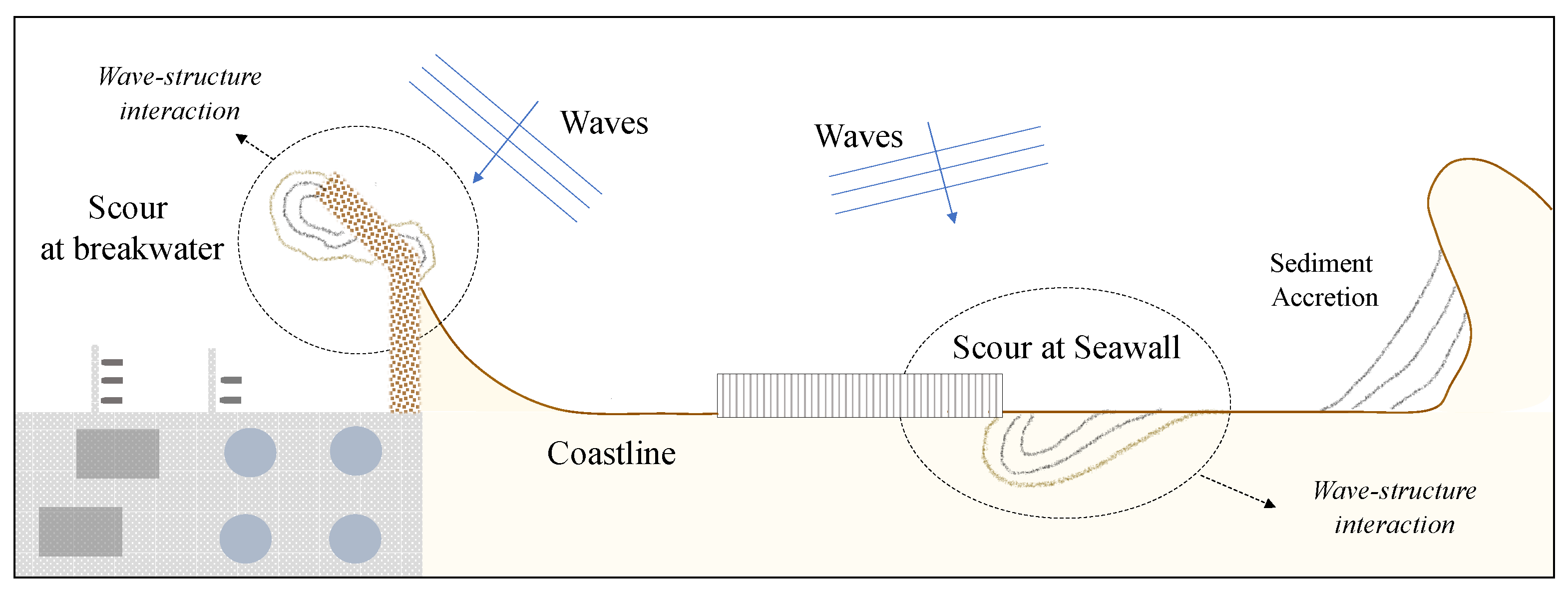
2.1. Concept of Scour

The presence of the protection structure changes the flow patterns in its immediate vicinity, inducing wave reflection and breaking, turbulence, and liquefaction [34]. These processes increase the fluid shear stress at the bottom (${\tau }_{f,b}$) and cause transport when a critical value (${\tau }_{cr,s}$) is reached. Increased local sediment transport leads to one of the greatest problems for coastal regions and marine structures: scour [35,36]. Scour around coastal structures is the additional erosion that takes place due to hydrodynamic forces acting on the seabed (Figure 1).

Scour has significant impacts on the economic and service life of many coastal structures [21]. Figure 2 shows an example of scour-induced damage at sloping structures. When scour undermines the structure, it cannot support the armour layer of a breakwater, which then slides and loses the fill material. Scour also impacts vertical-front caissons of breakwaters and other gravity structures (Figure 2). Seawalls can also settle and collapse as a result of scour. More details on scour around such structures can be found in the textbooks of Whitehouse [36] and Sumer and Fredsoe [34].

Damage to structures is not the only consequence of seabed scour. In fact, the presence of coastal structures can accelerate the erosion (and deposition), thus degrading coastlines [37,38,39], as shown in Figure 1. These examples of structural collapse or a loss of material along the coastline result from both transformation and interaction processes between marine dynamics, especially waves, and the coastal structure.

2.2. Processes Involved in Wave-Structure-Seabed Interactions

It is necessary to identify the physical processes contributing to the scour in order to properly design maritime protection structures and predict the final response of the seabed. A state-of-the-art review on scour processes has been presented in Sutherland et al. [18], Whitehouse [35], Sumer and Fredsøe [40]. The reviewed works complement and considerably extend the understanding of the governing processes for certain structures. According to these references, the processes that lead to scour are (acting singularly or in combination):

(A)

Wave energy transformation by its interactions with the structure [3,41,42]:

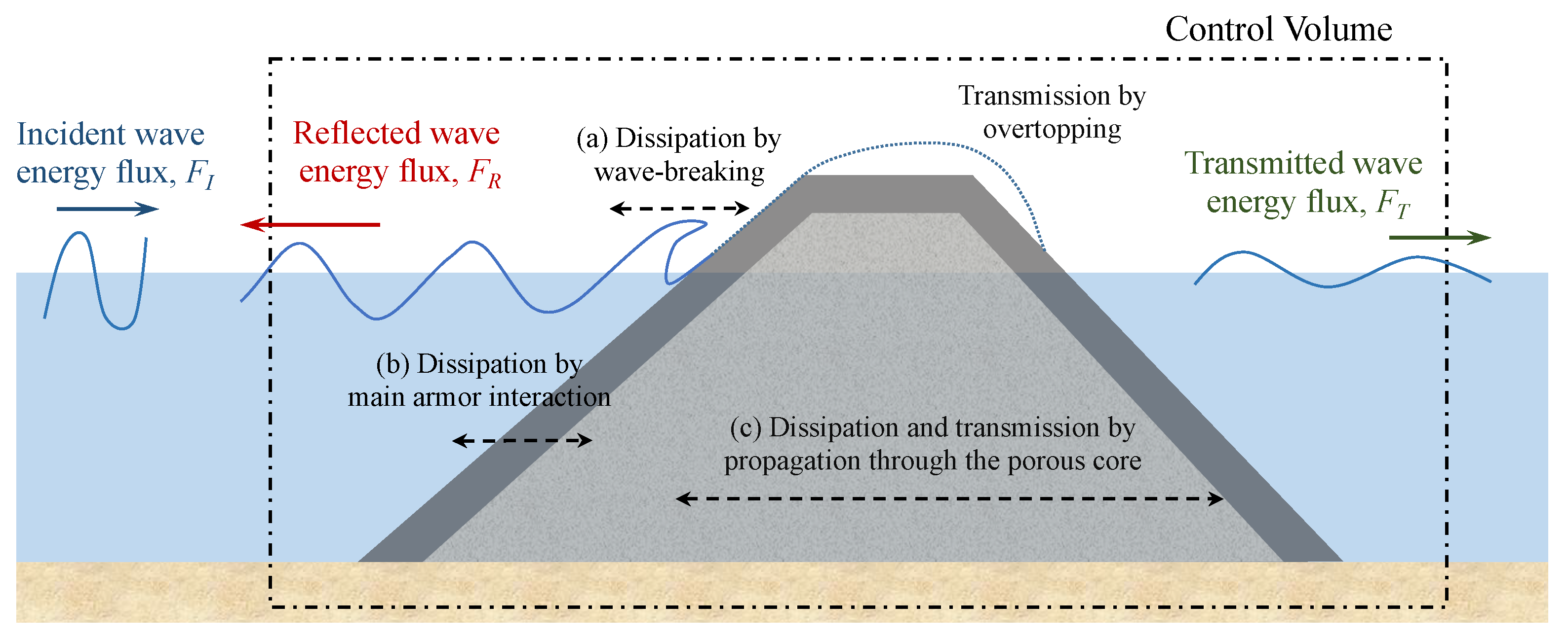
• Wave reflection: sediment transport due to wave reflection is perhaps the most commonly cited process in structure–seabed interactions [43]. The presence of a maritime structure transforms the incident wave energy into reflected energy, which is returned to the sea (Figure 3). This process involves an increase in wave height and wave energy, in front of the structure, i.e., greater shear stresses on the seabed and, thus, sediment transport.
• Wave dissipation: when waves impact a coastal structure, part of its incident wave energy is dissipated by (Figure 3): (a) wave-breaking on the slope or wall, (b) turbulent interactions (circulation and friction) with the armour layer, and (c) wave propagation through the porous media of the structure [44]. Among these, wave-breaking on the wall or slope mainly affects sediment transport, which generates turbulence in front of the structure and then mobilizes sediment.

(B)

Wave diffraction and refraction: when waves interact with an obstacle or coastline, part of the incident energy is concentrated or dispersed in a certain direction, which induces variations in the wave height and flow velocity, causing non-uniform erosion or sediment deposition [45,46]. Furthermore, waves that interact with submerged breakwaters are reduced by a number of energy dissipation mechanisms, including wave breaking and frictional dissipation [47,48], which can cause sediment transport around these structures.

(C)

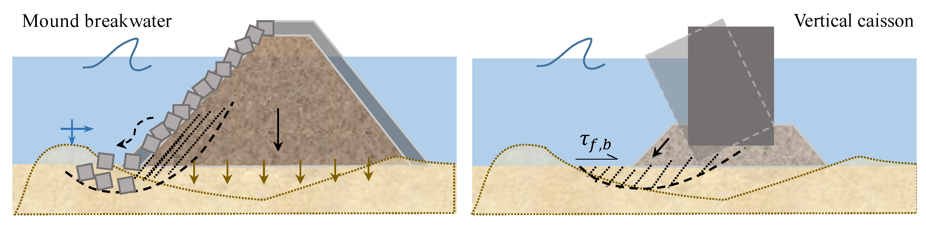
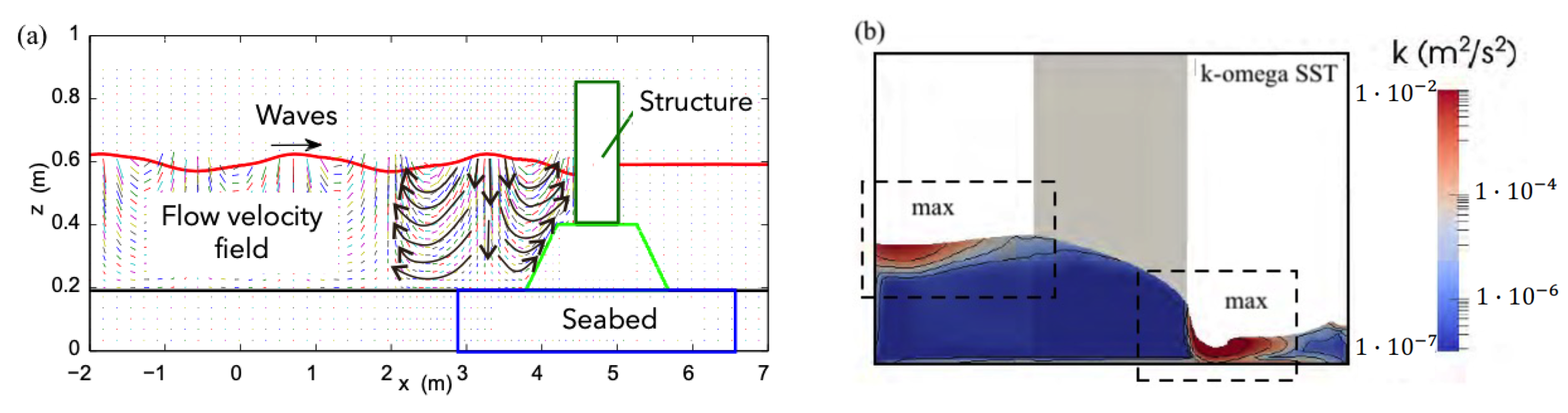
Turbulent flow around the structure: the flow contraction and velocity field generate turbulence and vortexes around and in front of the structure (Figure 4), which increase the bottom shear stresses (${\tau }_{f,b}$) and sediment mobilization [34,43]. Some figures of Higuera et al. [49] show the increase of turbulence kinetic energy ($k=\frac{u^2+v^2+w^2}{2}$) in front of and around a vertical wall and a porous breakwater.

(D)

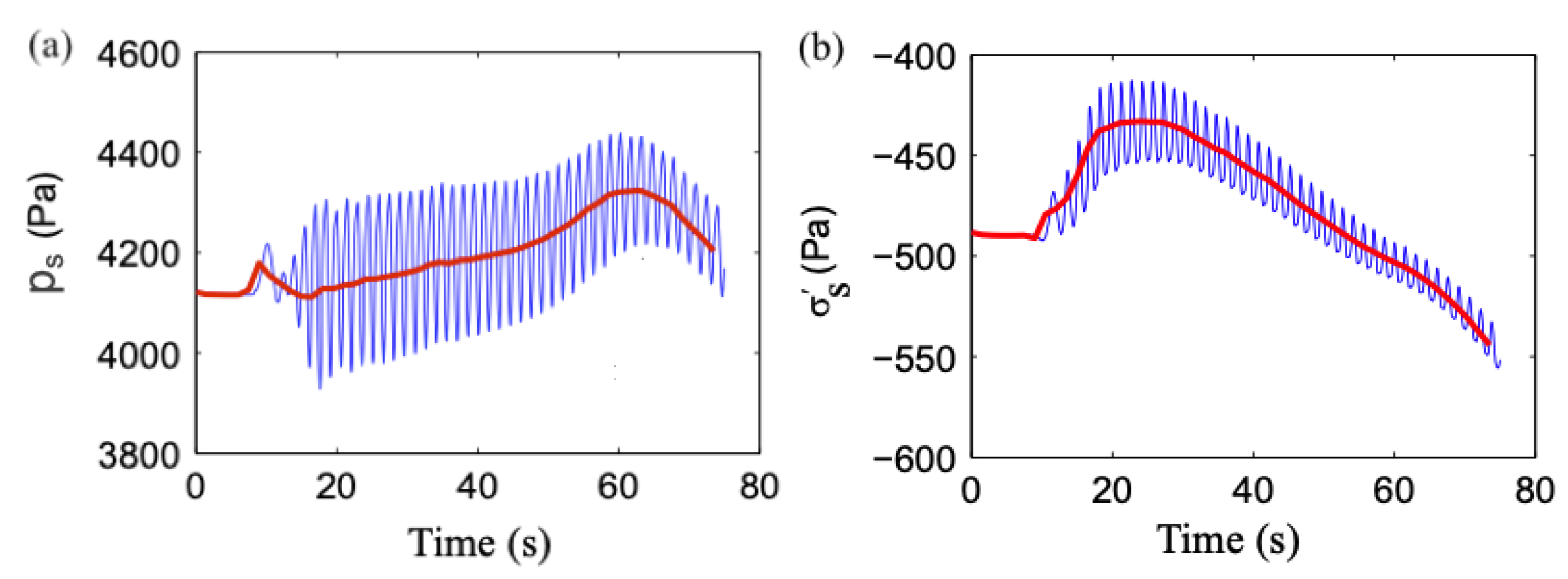
Liquefaction: the pressure differential in the soil may produce the liquefaction of the seabed [13,50,51], which leads to the loss of the seabed load-bearing capacity. A liquefied soil will be more susceptible to scour. The liquefaction phenomenon happens when the soil effective stresses are cancelled due to an increase of the pore water pressure. Figure 5 shows the stress field and pore pressure in front of a maritime structure. It can be seen how the effective normal stress (${\sigma }_s^{\prime }$) decreases as the wave-induced pore pressure ($p_s$) increases.

Figure 3. The wave energy transformation by its interactions with a maritime structure. The analysis of the wave energy transformation modes can be achieved by defining a finite control volume (CV) with a unit width and constant depth that includes the structure. The wave energy conservation equation in the control volume is given by $F_I-F_R-F_T-D^{{}^{\prime }*}=0$ [52], with $F_i$, $i=I$, R, and T being the mean energy flux of the incident, reflected, and transmitted wave trains, respectively; and, $D^{{}^{\prime }*}$ the mean bulk dissipation.

Figure 3. The wave energy transformation by its interactions with a maritime structure. The analysis of the wave energy transformation modes can be achieved by defining a finite control volume (CV) with a unit width and constant depth that includes the structure. The wave energy conservation equation in the control volume is given by $F_I-F_R-F_T-D^{{}^{\prime }*}=0$ [52], with $F_i$, $i=I$, R, and T being the mean energy flux of the incident, reflected, and transmitted wave trains, respectively; and, $D^{{}^{\prime }*}$ the mean bulk dissipation.

Figure 4. (a) The flow velocity increases around a composite vertical breakwater; (b) the turbulence kinetic energy ($k=\frac{u^2+v^2+w^2}{2}$) increases at the toe of the seawall. Both of the figures are adapted from the numerical simulations to study the interactions between ocean waves and maritime structures performed by Ye et al. [53] and Higuera [54], respectively.

Figure 4. (a) The flow velocity increases around a composite vertical breakwater; (b) the turbulence kinetic energy ($k=\frac{u^2+v^2+w^2}{2}$) increases at the toe of the seawall. Both of the figures are adapted from the numerical simulations to study the interactions between ocean waves and maritime structures performed by Ye et al. [53] and Higuera [54], respectively.

Figure 5. (a) The temporal evolution of the wave induced pore pressure, $p_s$; (b) effective normal stress of the soil in front of a composite vertical breakwater, ${\sigma }_s^{{}^{\prime }}$ (adapted from Ye et al. [53]).

Figure 5. (a) The temporal evolution of the wave induced pore pressure, $p_s$; (b) effective normal stress of the soil in front of a composite vertical breakwater, ${\sigma }_s^{{}^{\prime }}$ (adapted from Ye et al. [53]).

3. Numerical Modelling of Seabed Response

This section presents the governing equations and general methodology of three main Eulerian approaches, in this paper called (i) simple approach (Section 3.1), (ii) Biot approach (Section 3.2), and (iii) full multiphase approach (Section 3.3), for modelling the sediment transport and, thus, the seabed response around maritime structures. The numerical approaches attempt to capture the processes that are involved in the interactions of waves with the structure and their consequences on the seabed foundation. Figure 6 shows a general outline of the numerical approaches described hereafter, which are based on the Reynolds-Averaged Navier–Stokes (RANS) equations (the mass and momentum conservation equations) for the wave–structure interactions and mainly differ in the way that they model the seabed behaviour. This section also shows the applicability and summarizes the performance and parameters used for each numerical methods.

3.1. Simple Approach

The simple approach decomposes the wave–structure–seabed problem into three modules: (1) wave propagation and transformation with the structure, (2) bed load and suspended sediment transport, and (3) bed morphological changes. Figure 7 shows a summary diagram of the modules, parameters, and the interactions between modules. A detailed description of the modules is given below.

3.1.1. Wave-Structure Module: Rans Equations

The incompressible Reynolds-Averaged Navier–Stokes (RANS) equations are applied as the governing equations of fluid flow. These are time-averaged conservation equations of mass and momentum, which describe the mean flow field, respectively:

$$\frac{\partial u_{f,i}}{\partial x_i}=0$$

(1)

$$\frac{\partial u_{f,i}}{\partial t}+u_{f,j}\frac{\partial u_{f,i}}{\partial x_j}=-\frac{1}{\rho }\frac{\partial p_f}{\partial x_i}+\frac{\partial }{\partial x_j}\left[(\nu +{\nu }_T)\left(\frac{\partial u_{f,i}}{\partial x_j}+\frac{\partial u_{f,j}}{\partial x_i}\right)\right]+g_i$$

(2)

where the sub-indexes i, j = 1, 2, and 3 represent the x-, y-, and z-directions, respectively; f represents the fluid-phase; $u_f=(u_{f,x},u_{f,y},u_{f,z})$ is the fluid velocity; $p_f$ is the pressure; ${\rho }_f$ is the fluid density; $\nu =\mu /{\rho }_f$ is the fluid kinematic viscosity (being $\mu$ the dynamic viscosity); ${\nu }_T$ is the turbulent/eddy viscosity; and $g_i=(0,0,-g)$ is the gravitational acceleration. Equations (1) and (2) have the following considerations:

• The resulting flow variables (e.g., $u_f$, $p_f$) describe the mean flow field. Turbulence effects are introduced via the Reynolds’s stresses in the momentum equation, which must be modelled using a turbulence closure.
• The turbulence models are usually based on the Boussinesq’s eddy viscosity hypothesis: ${\nu }_T\left(\frac{\partial u_{f,i}}{\partial x_j}+\frac{\partial u_{f,j}}{\partial x_i}\right)$. The eddy viscosity ${\nu }_T$ is estimated using semi-empirical models.
• The free-surface of the waves and flow inside the porous media of the structure should be considered in this module.
• Density variations are considered in some instances. In this case, an extra density-weighted averaging step is carried out, which results in the Favre-Averaged Navier–Stokes equations (FANS).

Turbulence Model

This review paper does not focus on the different turbulence models and Blondeaux et al. [55] provides a detailed description of the flow–structure by comparing various turbulence models. However, it should be noted that, in the study of wave–structure–seabed interactions, the most appropriate turbulence model should provide an accurate description of (i) the flow close to the bottom (seabed surface) to obtain a reliable evaluation of the sediments transported by the flow [56] and (ii) the turbulent flow generated by the interactions with the structure. The turbulence models used in the papers cited in this work are summarized in Section 3.1.4, Section 3.2.2, and Section 3.3.2, respectively.

Free-Surface Capturing

Capturing the free surface is essential for modelling wave motion and wave-breaking. The Volume Of Fluid (VOF) technique is one of the most common methods to track the free surface location [54,57]. This method determines the phase within each cell in the domain by introducing an indicator function, $\varphi$ ($\varphi =1$ full of water, $\varphi =0$ full of air, interface $0<\varphi <1$), and solves the momentum equation (Equation (2)) for a pseudo fluid whose properties are weighted sums based on $\varphi$. The distribution of $\varphi$ is determined by solving a simple VOF advection equation:

$$\frac{\partial \varphi }{\partial t}+\frac{\partial \left(\varphi u_{f,i}\right)}{\partial x_i}=0$$

(3)

An alternative interface capturing method is the Level Set Method (LSM) that was proposed by Osher and Sethian [58], in which the interface is implicitly represented by the zero level set of a smooth signed distance function that adopts negative values in a phase, zero in the interphase, and positive values in the other phase. The evolution of this function is captured using a conservation equation that is similar to Equation (3), but an interface thickness is predefined. Across this region, a Heaviside function is used to smooth sharp flow variable changes and ensure numerical stability. In comparison with the VOF method, the LSM is more accurate in the capture of high curvature interfaces. However, it is not capable of ensuring mass conservation, which is a major drawback in comparison with the VOF method [59].

Flow inside the Permeable Structure

If the coastal structure is permeable, i.e., formed by a porous material, then the numerical approach should calculate the flow inside the porous media. In this case, the RANS equations need an additional volume-based averaging step to account for low porosity materials, $n\in$ (0.35–0.65) (being n, the porosity of the permeable structure), such as those that are normally found in coastal engineering structures. Hence, RANS equations are integrated into a porous control volume, obtaining the Volume-Averaged Reynolds-Averaged Navier–Stokes equations (VARANS) [49,60]:

$$\frac{\partial }{\partial x_i}\frac{u_{f,i}}{n}=0$$

(4)

$$\begin{array}{c}\hfill \frac{\partial u_{f,i}}{\partial t}+u_{f,j}\frac{\partial }{\partial x_j}\frac{u_{f,i}}{n}=-\frac{n}{\rho }\frac{\partial p_f}{\partial x_i}+n\frac{\partial }{\partial x_j}\left[(\nu +{\nu }_T)\left(\frac{\partial }{\partial x_j}\frac{u_{f,i}}{n}+\frac{\partial }{\partial x_i}\frac{u_{f,i}}{n}\right)\right]+n{g}_i\\ \hfill -a{u}_{f,i}-b{u}_{f,i}\left|u_{f,i}\right|-c\frac{\partial u_{f,i}}{\partial t}\end{array}$$

(5)

$$\frac{\partial \varphi }{\partial t}+\frac{\partial }{\partial x_i}\frac{\varphi u_{f,i}}{n}=0$$

(6)

Equations (4)–(6) are the mass, momentum, and phase volume fraction conservation equations inside the porous media, respectively. After volume averaging, three new terms appear on the right hand side of Equation (5), which are closure terms to account for the frictional and pressure forces, as well as the added mass of the individual components of the porous media. These three terms are drag forces that characterize the flow through the porous media [61]: the linear term (laminar flow), $a{u}_{f,i}$; the quadratic term (turbulent flow), $b{u}_{f,i}\left|u_{f,i}\right|$; and, the inertial acceleration (unsteady flow) term $c\frac{\partial u_{f,i}}{\partial t}$. The coefficients a, b, and c depend on the physical properties of the material and control the balance between each of the friction terms [62,63].

Note that, for impermeable structures, a non-slip ($u_f=0$) boundary condition is imposed on the structure surface and the governing equations in the wave–structure module in the case of RANS equations.

3.1.2. Sediment Transport Module

This module includes the calculation of the bed load and suspended sediment transport. Numerous bed load equations have been developed over the past century, $q_B$. The formulas are often empirical and they are commonly based on excess shear stress, where the shear stress is greater than the critical value for incipient motion (${\tau }_{b,f}>{\tau }_{cr,s}$). Bedload equations can include parameters for the characteristics of the fluid and the seabed, such as bed-forms (flat bed or ripples), slope, and sediment composition [64,65,66]. Common variables include:

$$q_B=f({\tau }_{f,b},d_{50},{\rho }_s,{\tau }_{cr,s})$$

(7)

with ${\tau }_{f,b}$ the bottom shear stress of the fluid (from the wave–structure module); ${\tau }_{cr,s}\sim d_{50}({\rho }_s-{\rho }_f)g$, the critical bed shear stress; and, $d_{50}$ and ${\rho }_s$, the characteristic diameter and density of the sediment, respectively.

For the suspended sediment transport, the suspended concentration ($c_s$) is often calculated by the advection–diffusion equation (Equation (8)) [67,68], but other papers use empirical formulas for $c_s$ as Ahmad et al. [69], who used the empirical formula of Rouse [70]; and, others used empirical formulas for the total sediment transport load (bed and suspended), such as Tofany et al. [71,72].

$$\frac{\partial c_s}{\partial t}+u_{f,i}\frac{\partial c_s}{\partial x_i}+w_s\frac{\partial c_s}{\partial x_3}=\frac{\partial }{\partial x_i}\left(D_T\frac{\partial c_s}{\partial x_i}\right)$$

(8)

where $w_s$ is the settling velocity of the sediment, whose expression is empirical and depends on the hindering settling effects. $D_T$ is the diffusion coefficient, normally related with the eddy viscosity, ${\nu }_T$ (from the wave–structure module) [56,73], and $u_f$ is the flow velocity (from the wave–structure module). Concerning the suspended concentration, the suspended load transport is calculated by:

$$q_S={\int }_z{u}_{f,x}{c}_{s}dz$$

(9)

3.1.3. Morphological Bed Module

The evolution of the seabed profile is obtained with the Exner formula. It is based on the sediment local mass balance and it involves a non-linear propagation of the bed-level deformation in the direction of the sediment transport and the spacial variation of the sediment fluxes between the bed load and suspended load [69]. The equation is defined as:

$$\frac{\partial h_s}{\partial t}+\frac{1}{1-n_s}\left(\frac{\partial q_{t,i}}{\partial x_i}\right)+E-D=0$$

(10)

where $q_t=q_B+q_S$ is the total load transport; $n_s$ is the seabed porosity; and, the term $(E-D)$ defines the net sediment movement of the suspended load [74]. Here, E and D are the erosion and deposition rates, whose expressions depend on the settling velocity, $w_s$, and the volumetric reference concentration at the bed ($c_b$).

3.1.4. Applicability of the Simple Approach

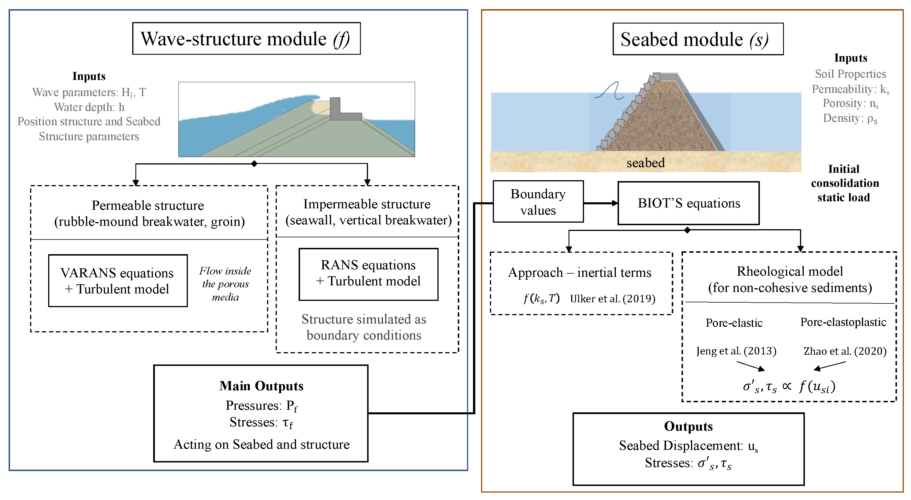
This numerical method is referred to as the simple approach in this paper, because the seabed behaviour is modelled using empirical equations, which are relatively easier to implement in comparison with the other approaches. The simple approach is used, in particular, for estimating the scour around structures with low weight-structure load on the seabed, such as submarine pipelines. Some of the most recent and outstanding studies that used the simple approach for estimating the scour around structures are: Ahmad et al. [69], who investigated the local scour around a composition of pile structures (Figure 8), and, Ahmad et al. [75], who presented the numerical approach for studying scour due to wave impacts on a vertical wall. They showed that the wave-breaking and impact on the structure govern the different stages of the scour formation. Baykal et al. [76] also investigated the flow and scour around a vertical pile. Seabed deformation was modelled while using the mesh deformation technique, which allowed for showing the development of turbulent structures in the wake of the monopile, such as horseshoe vortices. Furthermore, Chen [77] developed a Lagrangian–Eulerian model based on the two-dimensional (2D) Navier–Stokes equations for the wave field, and a bed load sediment transport and morphological model to simulate the scouring process in front of a vertical-wall. Their results tend to underestimate the scouring rate. Gislason et al. [78] calculated the 2D flow and sediment transport in front of a breakwater, coupling a morphological model with Navier–Stokes equations. Their results do not show the seabed movement in detail, a drawback of the simple modelling approach. Li et al. [79] investigated the 2D local scour beneath two submarine pipelines in tandem based on the calculation of the bed/suspended load transport and the morphological changes of the seabed. This work investigated the scour around the pipelines under wave–current conditions. Omara et al. [80] simulated the scour processes, both hydrodynamically and morphologically, around vertical and inclined piers in a new version of FLOW-3D that estimates the motion of sediment transport (suspended, settling, entrainment, and bed load). Tofany et al. [71,72] studied the effects of breakwater steepness and wave overtopping on the scouring process in front of impermeable and vertical breakwaters. They used a 2D RANS-VOF model with additional bottom shear stresses in the momentum equations, coupled with turbulence closure, sediment transport load, and morphological model. Klonaris et al. [81] presented the numerical and experimental results of the evolution of a sandy beach in a surf-zone around a permeable submerged breakwater. They used the Boussinesq-type equations instead of Navier–Stokes equations to simulate wave propagation over a porous bed, coupled with a sediment transport module, including both bed and suspended loads.

Table 1. A summary of the most recent and leading works that use the simple approach to model the wave–structure–seabed interactions.

Author	Year	Approach NS	Phases	Coupling	Interface Capture	Morphological Change	Turbulence Closure	Comments
Ahmad et al. [69]	2020	RANS	Water-sediment	Two-way	None	LSM	$k-\omega$
Li et al. [79]	2020	RANS	Water-sediment	Two-way	None	LSM	$k-\omega$	Morphological model mesh variation
Klonaris et al. [81]	2020	Boussinesq equation	Water-sediment	One-way	None	None	None	Different governing eqs for the wave module
Ahmad et al. [75]	2019	RANS	Air-water-sediment	Two-way	LSM	LSM	$k-\omega$
Baykal et al. [76]	2017	RANS	Water-sediment	Two-way	None	Mesh deformation	$k-\omega$	Mesh deforms based on depositions - Exner’s Equation
Tofany et al. [71]	2014	RANS	Air-water-sediment	One-way	VOF	None	$k-ϵ$	Simple model in Matlab. Turbulent model used not suitable for bottom boundary layer

provides a summary of the parameters and performance of the simple model for some of the relevant studies cited. In general, these focus on water-seabed interactions. Thus, they often disregard the air flow. The RANS equations for the liquid phase are solved using the $k-\omega$ model of Wilcox et al. [83] as turbulence closure model, which is considered to be a better choice for solving the boundary layer over the other two-equation turbulence models. Wave action is often imposed using source terms on the corresponding wave generating boundary. In some studies, the seabed deformation is accounted for using an interface tracking method [69,84]. The Level Set Method (LSM) [58] is the most common method in this regard, which is considered to be more accurate and stable when dealing with high curvature interfaces than the VOF method. Note that Baykal et al. [76] used a mesh deformation technique, which might be more accurate, but it is noticeably more expensive from a computational perspective. Seabed deformation (either using an interface tracking method or mesh deformation) allows for two-way coupling between the fluid region and seabed. This is often not the case in other more complex approaches, such as the RANS–Biot combination. In general, although the results of these studies are considered to be acceptable, they tend to underestimate the scouring rate and do not show the seabed movement in detail. Moreover, there is no consensus regarding the choice of empirical formulas for the seabed module.

3.2. Biot Approach

An alternative to the simple method for describing wave-–seabed interactions around marine structures is to combine Biot theory [85] (see Equations (11)–(13)) with the Navier–Stokes (NS) equations for the wave field. This numerical approach studies the wave–structure–seabed interactions with two modules: (1) the wave–structure module, based on RANS or VARANS equations as with the simple approach (see Section 3.1.1), and (2) the seabed module (described below) in which the Biot’s equations govern the dynamic response of the porous seabed under wave loading. Figure 9 presents a summary of the modules that are presented in this numerical approach.

3.2.1. Seabed Module: Biot’s Equations

The Biot’s equations are adopted as the governing equations for describing the dynamic response of the isotropic porous seabed under wave loading [85]. This paper provides a brief outline of the Biot’s equations, but further details can be found in Jeng and Ou [86].

(1)

The momentum conservation equation for the mixture (fluid and sediment) can be written as:

$$\left(\frac{\partial {\sigma }_{s,i}^{\prime }}{\partial x_i}+\frac{\partial {\tau }_{s,ij}}{\partial x_j}\right)+\rho g_i=\rho \frac{{\partial }^2{x}_{s,i}}{\partial t^2}+{\rho }_f\frac{{\partial }^2{w}_{f,i}}{\partial t^2}$$

(11)

(2)

When considering the flow to be governed by Darcy’s law, the momentum equation of fluid phase is written as:

$$-\frac{\partial p_s}{\partial x_i}+{\rho }_f{g}_i={\rho }_f\frac{{\partial }^2{x}_{s,i}}{\partial t^2}+\frac{{\rho }_f}{n_s}\frac{{\partial }^2{w}_{f,i}}{\partial t^2}+\frac{{\rho }_f{g}_i}{k_s}\frac{\partial w_{f,i}}{\partial t}$$

(12)

(3)

The mass conservation equation for fluid phase can be stated as;

$$\frac{\partial }{\partial t}\left(\frac{\partial x_{s,i}}{\partial x_i}\right)+\frac{\partial }{\partial t}\left(\frac{\partial w_{f,i}}{\partial x_i}\right)=-\frac{n_s}{K_f}\frac{\partial p_s}{\partial t}$$

(13)

In these equations, ${\sigma }_s^{\prime }$ and ${\tau }_s$ are the effective normal and shear stresses of the soil, respectively; $p_s$ is the wave-induced oscillatory pore pressure; $x_s=(x_{s,x},x_{s,y},x_{s,z})$ is the seabed displacement; $w_f$ is the averaged (Darcy) fluid velocity; $k_s$ and $n_s$ are the permeability and porosity of the seabed, respectively; $\rho ={\rho }_f{n}_s+{\rho }_s(1-n_s)$ is the total density; and, $K_f$ is the bulk modulus of pore water that is related with the degree of saturation of the seabed, $S_r$. For this module, there are two considerations to be taken into account: (i) the inertial terms and (ii) the rheological model that relates the stresses and deformation of the seabed under wave action.

Inertial Terms

Different expressions for the Biot’s equations are implemented, depending on the rate of wave loading (wave period, $T_w$) and the characteristics of the porous media (permeability, $k_s$) [87,88,89]:

• Fully dynamic: the coupled equations of flow and deformation are formulated to include both acceleration terms: $\frac{{\partial }^2{x}_{s,i}}{\partial t^2}$, $\frac{{\partial }^2{w}_{f,i}}{\partial t^2}$
• Partly dynamic, which is also known as $u-P$ dynamic: the coupled equations of flow and deformation are formulated when only considering the acceleration of the seabed, $\frac{{\partial }^2{x}_{s,i}}{\partial t^2}$.
• Quasi-static: both inertial terms are ignored, resulting in quasi-static coupled flow and deformation formulation.

Rheological Models

The response of the wave–seabed interactions can be evaluated by rheological models, which relate the normal and shear stresses, (${\sigma }_s^{\prime }$, ${\tau }_s$), and the strain, ${ϵ}_s=\frac{\partial x_{s,i}}{\partial x_i}$, of the soil under the cyclic wave action. Most of the works analyse the wave–structure interactions on non-cohesive seabeds, i.e., composed by sands and/or gravels. For cohesive seabeds (silts and clays), the lack of laboratory or field tests makes it difficult to calibrate and validate the numerical models. A detailed description of rheological models for cohesive and non-cohesive soils is given in Díaz-Carrasco [90].

Most of the papers study the seabed response that is composed of non-cohesive sediments that behave primarily as elastic materials that, in contact with water, have a pore-elastic (dense seabed) [91,92] or pore-elastoplastic (loose seabed) behaviour [86,93,94,95].

Interactions between the Modules

The steps to interact the results of the wave–structure module with the seabed module are the following:

1.

The wave-induced pressure and bottom shear stresses determined in the wave module are the boundary conditions for the seabed module: $p_s=p_f$ and ${\tau }_{f,b}={\tau }_s$ at the seabed surface.

2.

The initial consolidation state of the seabed due to static wave and structure loading has to be determined before the dynamic wave loading is applied in the numerical model. This initial consolidation state of the seabed will be the initial stress state for the dynamic seabed response under wave loading.

3.

The seabed’s feedback effect on the wave and structure motions (two-way coupling) is neglected.

3.2.2. Applicability of the Biot Approach

There are many studies that use this approach for estimating the seabed movement around maritime structures, in particular breakwaters. Their results focus more on the mechanical behaviour (stress field and pressure) of the bearing seabed under wave loading and its interactions with the structure. Jeng et al. [91], Zhang et al. [96,97], Zhao et al. [98] studied the response of the porous seabed around a permeable breakwater while using the VARANS equations that were coupled with the dynamic Biot equations for a porous elastic seabed, and Zhang et al. [99] around a submarine pipeline. He et al. [100], Ye et al. [101] used the integrated numerical model FSSI-CAS 2D with VARANS equations and the dynamic Biot equations that were developed by Ye et al. [102] for studying the harbour zone of Yantai port in China as an engineering case. Zhao and Jeng [92] developed an integrated model (VARANS equations coupled with Biot equations) to investigate the wave-induced sloping seabed response in the vicinity of breakwaters. Their numerical results showed that the breakwater permeability, density, and slope of the seabed significantly affect the potential liquefaction, which leads to scour effects (Figure 10). Ye et al. [93], Zhao et al. [95] used the same approach to study the wave–structure–seabed interactions. They modelled the relation between stresses and deformation of the seabed with a poro-elastoplastic behaviour. Lin et al. [103,104], Zhao et al. [105] investigated the seabed response around a mono-pile foundation simulating the wave field with two-phase incompressible RANS equations and a wave-induced dynamic seabed response with a quasi-static version of the Biot equations. More recently, Jeng et al. [106] developed a combined approach that solved the Biot equations using a Radial Basis Function method to investigate the wave-induced soil response around a submerged breakwater. This method is meshless, which simplifies the solution of the seabed region and allows its application to larger configurations, such as around offshore pipelines Wang et al. [107]. Li et al. [84] developed an open-source numerical toolbox for modelling the porous seabed interactions with waves and structures in the finite-volume-method (FVM)-based OpenFOAM framework. This toolbox incorporates the incompressible Navier–Stokes equations for the wave module and the Biot equations for the seabed module considering the anisotropic seabed characteristics. Li et al. [108] studied the wave-induced seabed response and liquefaction risk around a hexagonal gravity-based offshore foundation. As can be seen, the abundance of works regarding the application of the RANS–Biot approach demonstrates its viability for estimating the scour around relatively large structures. Although most of them limit impermeable structures and its results focus on the stress state and pressure on the seabed. In fact, these works generally study the liquefaction phenomenon that is induced by wave action and how it affects the structure.

Table 2. A summary of the most recent and leading works that use the RANS–Biot approach to model the wave–structure-seabed interactions.

Author	Year	Approach NS	Phases	Coupling	Interface Capture	Turbulence Closure	Inertial Terms	Rheological Model	Comments
Jeng et al. [106]	2021	VARANS	Air-water- -sediment-structure	One-way	VOF	Not specified	u-p	Poro-elastic	Used a Radial Basis Function method to model the sediment (meshless method)
Zhao et al. [95]	2020	VARANS	Air-water-sediment	One-way	VOF	$k-ϵ$	u-p	Poro-elastoplastic
Li et al. [84]	2020	RANS	Air-water-sediment	One-way	VOF	Not specified	u-p	Orthotropic poro-elastic	Anisotropic soil characteristics
Zhao et al. [105]	2017	RANS	Air-water-sediment	One-way	VOF	$k-ϵ$	u-p	Poro-elastic
Ye et al. [94]	2017	RANS	Air-water-sediment	One-way	VOF	Not specified	u-p	Poro-elastoplastic	3D domain with an impermeable breakwater
Elsaftu and Oumeraci	2016	VARANS	Air-water-sediment	One-way	VOF	Not specified	Full u-p quasi-static	Poro-elastoplastic
Lin et al. [103]	2016	RANS	Air-water-sediment	One-way	LSM	$k-ϵ$	Quasi-static	Poro-elastic	Used Finite Element Method
Zhao and Jeng [92]	2015	VARANS	Water-sediment	One-way	-	$k-ϵ$	Quasi-static	Poro-elastic	Add a phase-resolved shear stress model that accounts for oscillatory mechanisms
Ye et al. [93]	2015	VARANS	Air-water- -sediment-structure	One-way	VOF	$k-ϵ$	u-p	Poro-elastoplastic	Improved sediment modelling
Jeng et al. [91]	2013	VARANS	Air-water-sediment	One-way	VOF	k model	u-p	Poro-elastic

summarizes the performance and parameters for developing the RANS–Biot approach of the most relevant studies found. These are noticeably more common in the literature than the other two approaches, which shows its good compromise with regards to accuracy versus complexity. Most of these studies consider the effects of wave breaking and wave–structure interactions, for which they use the VARANS equations in combination with the VOF method. Moreover, the standard $k-ϵ$ model is often chosen for turbulence closure. This approach does not consider seabed effects on the fluid phase (one-way coupling), as mentioned above. Most of these studies use the $u-p$ approximation for the inertial terms in the Biot’s equations, which offers improved results over the quasi-static formulation [88]. Elsafti and Oumeraci [109] observed that this approximation significantly reduces the computational time, and it should be considered whenever pore fluid acceleration is negligible. Otherwise, the fully-dynamic formulation is recommended.

3.3. Full Multiphase Approach

The movement of sediments due to the fluid flow is a two-phase phenomenon [110]. The starting point for developing any multiphase model is the local instantaneous formulation, which consists of field equations that are applied to the distinct phases complemented with jump conditions to match the solution at the interface and source terms to account for interactions between phases.

3.3.1. Governing Equations

The governing equations for multiphase models are the conservation equations of mass and momentum for each phase. Generally, the system is simplified using a pseudo-fluid approach for the water–air region in combination with a free surface capture method (see Section 3.1.1). A specific momentum equation is used for the sediment (solid phase). However, specific continuity equations are necessary for each phase since the system now includes three phases. The final mass and momentum conservation equations are written as,

(1)

Mass conservation equations:

$$\frac{\partial c_s}{\partial t}+\frac{\partial \left(c_s{u}_{s,i}\right)}{\partial x_i}=0;\mathrm{Sediment}\mathrm{phase}$$

(14)

$$\frac{\partial (1-c_s)\varphi }{\partial t}+\frac{\partial (1-c_s)\varphi u_{f,i}}{\partial x_i}=0;\mathrm{Water}\mathrm{phase}$$

(15)

$$\frac{\partial (1-c_s)(1-\varphi )}{\partial t}+\frac{\partial (1-c_s)(1-\varphi )u_{f,i}}{\partial x_i}=0;\mathrm{Air}\mathrm{phase}$$

(16)

(2)

Momentum conservation equations:

$$\begin{array}{c}\hfill \frac{\partial {\rho }_f(1-c_s)u_{f,i}}{\partial t}+\frac{\partial {\rho }_f(1-c_s)u_{f,i}{u}_{f,i}}{\partial x_i}={\rho }_f(1-c_s)g_i-(1-c_s)\frac{\partial p_f}{\partial x_i}\\ \hfill +\frac{\partial (1-c_s){\mathcal{T}}_f}{\partial x_j}-c_s{\rho }_s\frac{u_{f,i}-u_{s,i}}{{\tau }_p}+\frac{{\rho }_s}{{\tau }_p}\frac{(1-c_s)\nu }{S_c}\frac{\partial c_s}{\partial x_i};\mathrm{Fluid}\mathrm{phase}\end{array}$$

(17)

$$\begin{array}{c}\hfill \frac{\partial {\rho }_s{c}_s{u}_{s,i}}{\partial t}+\frac{\partial {\rho }_s{c}_s{u}_{s,i}{u}_{s,i}}{\partial x_i}={\rho }_s{c}_s{g}_i-c_s\frac{\partial p_f}{\partial x_i}-\frac{\partial c_s{p}_s}{\partial x_i}\\ \hfill +\frac{\partial c_s{\mathcal{T}}_s}{\partial x_j}-c_s{\rho }_s\frac{u_{f,i}-u_{s,i}}{{\tau }_p}+\frac{{\rho }_s}{{\tau }_p}\frac{(1-c_s)\nu }{S_c}\frac{\partial c_s}{\partial x_i};\mathrm{Sediment}\mathrm{phase}\end{array}$$

(18)

where the sub-indexes f and s refer to the fluid and sediment phases, respectively; $\rho$ is the density; c is the volume concentration of sediment; u is the velocity; $\nu$ is the kinematic viscosity; $S_c$ is the Schmidt number; p is the pressure; $\mathcal{T}$ represents the viscous and turbulent stress tensor; and, ${\tau }_p=\frac{{\rho }_s}{{\rho }_f-{\rho }_s}{(1-w_s)}^{2}g$ is the response time of the particles, with $w_s$ being the settling velocity of the sediment. The last two terms in the momentum equations are related to momentum interchanges between the sediment and fluid phases: the first term accounts for the drag force and the second term for turbulent dispersion.

3.3.2. Applicability of the Full Multiphase Approach

The application of the full multiphase model allows for greater accuracy regarding sediment movement and seabed–wave–structure response. In this case, the seabed region is modelled as a continuous medium, which provides greater detail in the description of pressure, stresses, and interchange terms between phases. This numerical approach is the most recent, but it has a high numerical complexity. For the high sediment concentration region (near the bed), the model requires a very refined mesh, which leads to a higher computational cost. The studies that are based on this approach mainly focus on small-scale problems that are related with the estimation of the sediment transport around small structures, such as monopiles.

Many models have been developed for the two phases, i.e., water-sediment [111,112,113,114,115,116], and few of them include air as a third phase to handle the free surface tracking. These studies mostly differ in the way they treat closure terms for particle stresses, turbulence, and momentum exchanges. In this regard, Hsu et al. [111] show that adding a turbulence modulation term due to particle presence to the $k-ϵ$ model improves the accuracy in the boundary layer. Given the grid requirements and complexity of the models, these are usually limited to 1D or 2D domains. Lee et al. [115] propose the inclusion of extra rheological terms that account for enduring-contact, as well as viscous and interstitial effects, which extend the range of application of their model to higher Reynolds numbers. Lee et al. [110] and Ouda and Toorman [117] used a three-phase model to study the local scour caused by a submerged wall jet and around a submarine pipeline. In both studies, the numerical results exhibited good agreement with the experimental data and the model was able to capture the key processes that govern the scour effect (Figure 11).

Table 3. Summary of the most recent and leading works that use the full multiphase approach to model the wave–structure–seabed interactions.

Author	Year	Approach NS	Coupling	Interface Capture	Turbulence Closure	Particle Stresses	Comments
Ouda and Toorman [117]	2019	FANS	Mixture model	Modified VOF	Modified $k-ϵ$	Dense granular flow Lee et al. [119]	Compared $k-ϵ$ and mixing length turbulence models
Cheng et al. [116]	2017	RANS	Two-way	None	Modified $k-ϵ$	Concentration dependent: - collisional theory - frictional component	Propose empirical turbulence modifications for flows with sediments
Lee et al. [110]	2017	RANS	Two-way	VOF	Modified $k-ϵ$	Lee et al. [115] plus in-house terms	Thorough closure of particle stresses
Lee et al. [115]	2016	FANS	Two-way	None	Modified $k-ϵ$ with Low Re corrections	Follows Lee et al. [119]	Alternative solution algorithm that prevents domain division
Amoudry et al. [114]	2008	RANS	Two-way	None	$k-ϵ$	Collisional theory	Propose empirical turbulence modifications for flows with sediments

proposes a summary of the performance and parameters of the most relevant studies using this approach. The multiphase approach requires turbulence modulation due to the presence of sediment particles. Hence, these studies generally use a modified $k-ϵ$ model. Moreover, momentum exchanges between phases are accounted for by using source terms in the momentum equations. Thus, this approach offers two-way coupling between the sediments and the water phase. Only one study considered a domain big enough to also include the air–water interface [117]. However, in this study, the authors simplified the system by using a mixture model, wherein a single system of continuity and momentum equations is used and the phase locations are tracked using a concentration marker. As can be seen, the use of a full multiphase approach requires the consideration of several closure terms for the particle stresses, turbulence stresses, and phase interaction mechanisms, most of which are based on empirical equations.

4. Conclusion and Future Prospects

The main objective of this paper is to present a comprehensive review of the numerical approaches for modelling the wave–structure–seabed interactions, while focusing on the seabed response, i.e., scour. This review is intended to complement the review papers on sediment transport and seabed response around maritime structures, which are mainly based on analytical and experimental studies. For this purpose, a literature review of the main and most recent works (over the last 10 years) on numerical modelling was carried out.

There are three main Eulerian approaches for modelling the sediment transport and the seabed response around maritime structures. In this paper, they are referred to as: (i) simple approach, (ii) Biot approach, and (ii) full multiphase approach. These three approaches are based on Reynolds-Averaged Navier–Stokes equations for the wave–structure module and they differ mostly in how they tackle the seabed module.

1.

The simple approach considers: (a) the bed load transport with empirical formulas; (b) the suspended concentration with the advection–diffusion equation and suspended load transport; and, (c) the seabed level with the Exner formula. The wave module is mainly based on RANS or VARANS equations, depending on whether the structure is permeable or impermeable. The studies that use the simple modelling approach mainly focus on small and low weight-structures to simulate the movement and deformation of the seabed (two-coupled approach). For large structures, such as breakwaters, these studies tend to underestimate the scouring results.

2.

The Biot approach involves the RANS or VARANS equations for the wave module and the Biot’s equations for the seabed module. Biot’s equations are used to obtain the seabed displacement and stresses. The wave model is responsible for the wave generation and propagation, and it determines the pressure, $p_f$, and stresses, ${\tau }_{f,b}$, acting on th seabed and marine structures. The outputs of the wave module are used as boundary conditions for the seabed module. The studies that used Biot’s equations for the seabed module focus more on the stress field and pressures, which is, the mechanical behaviour of the seabed.

3.

The full multiphase approach is the more complex approach and is difficult to implement numerically. It solves each phase (sediment, water, and air) with the Navier–Stokes equations (mass and momentum) at the same time and space. Most of the studies are based on small-scale problems given the very high computational costs that are associated with its use.

This paper describes the general concept and methodology of each numerical approach for modelling wave–structure–seabed interactions. However, there are certain aspects when developing a numerical model that need to be studied in more detail and that were not the focus of this review: (i) the turbulence model that best characterizes the near-bed turbulent flow–structure and the turbulent flow interactions with the structure; (ii) the particle stresses, which is, the rheological models that provides a functional relation between the stresses and strains of the seabed under wave action; and (iii) the optimal boundary and initial conditions for each numerical approach.

References

1. Vousdoukas, M.I.; Mentaschi, L.; Voukouvalas, E.; Verlaan, M.; Feyen, L. Extreme sea levels on the rise along Europe’s coasts. Earth’s Future 2017, 5, 304–323. [Google Scholar] [CrossRef]
2. Irie, I.; Nadaoka, K. Laboratory reproduction of seabed scour in front of breakwaters. In Coastal Engineering 1984; American Society of Civil Engineers: Reston, VA, USA, 1985; pp. 1715–1731. [Google Scholar]
3. Burcharth, H.; Hughes, S. Shore Protection Manual. Chapter 6: Fundamentals of design; US Army Corps of Engineers: Washington, DC, USA, 2002; Volume 1.
4. ROM 1.1-18. Recommendations for Breakwater Construction Projects; Technical Report; Puertos del Estado: Madrid, Spain, 2018. [Google Scholar]
5. Molinero Guillén, P. Large breakwaters in deep water in northern Spain. In Proceedings of the Institution of Civil Engineers—Maritime Engineering; Thomas Telford Ltd.: London, UK, 2008; Volume 161, pp. 175–186. [Google Scholar]
6. Puzrin, A.M.; Alonso, E.E.; Pinyol, N.M. Geomechanics of Failures; Springer Science & Business Media: Berlin, Germany, 2010. [Google Scholar]
7. Hughes, S. Scour and Scour Protection. Ph.D. Thesis, Coastal and Hydraulics Laboratory, US Army Engineer Research and Development Center, Vicksburg, MS, USA, 1993. [Google Scholar]
8. Sumer, B.M. Coastal and offshore scour/erosion issues-recent advances. In Proceedings of the 4th International Conference on Scour and Erosion (ICSE-4), Tokyo, Japan, 5–7 November 2008; pp. 85–94. [Google Scholar]
9. Maa, P.Y.; Mehta, A. Mud erosion by waves: A laboratory study. Cont. Shelf Res. 1987, 7, 1269–1284. [Google Scholar] [CrossRef]
10. Foda, M.A.; Hunt, J.R.; Chou, H.T. A nonlinear model for the fluidization of marine mud by waves. J. Geophys. Res. Ocean. 1993, 98, 7039–7047. [Google Scholar] [CrossRef]
11. Tsai, Y.; McDougal, W.; Sollitt, C. Response of finite depth seabed to waves and caisson motion. J. Waterw. Port Coast. Ocean Eng. 1990, 116, 1–20. [Google Scholar] [CrossRef]
12. Kumagai, T.; Foda, M.A. Analytical model for response of seabed beneath composite breakwater to wave. J. Waterw. Port Coast. Ocean Eng. 2002, 128, 62–71. [Google Scholar] [CrossRef]
13. Liao, C.; Tong, D.; Chen, L. Pore pressure distribution and momentary liquefaction in vicinity of impermeable slope-type breakwater head. Appl. Ocean Res. 2018, 78, 290–306. [Google Scholar] [CrossRef]
14. Sutherland, J.; Obhrai, C.; Whitehouse, R.J.; Pearce, A. Laboratory tests of scour at a seawall. In Proceedings of the 3rd International Conference on Scour and Erosion, Amsterdam, The Netherlands, 1–3 November 2006; Technical University of Denmark: Lyngby, Denmark, 2006. [Google Scholar]
15. Pearce, A.; Sutherland, J.; Obhrai, C.; Müller, G.; Rycroft, D.; Whitehouse, R. Scour at a seawall-field measurements and laboratory modelling. In Coastal Engineering, San Diego, California, USA, 3–8 September 2006; World Scientific: Singapore, 2007; Volumes 5, pp. 2378–2390. [Google Scholar]
16. Tsai, C.P.; Chen, H.B.; You, S.S. Toe scour of seawall on a steep seabed by breaking waves. J. Waterw. Port Coast. Ocean Eng. 2009, 135, 61–68. [Google Scholar] [CrossRef]
17. Jayaratne, R.; Mendoza, E.; Silva, R.; Gutiérrez, F. Laboratory Modelling of Scour on Seawalls. In Coastal Structures and Solutions to Coastal Disasters 2015: Resilient Coastal Communities; ASCE: Reston, VA, USA, 2017; pp. 809–816. [Google Scholar]
18. Sutherland, J.; Chapman, B.; Whitehouse, R. SCARCOST Experiments in the UK Coastal Research Facility-Data on Scour around a Detached Rubble Mound Breakwater; Technical Report; HR Wallingford: Oxfordshire, UK, 1999. [Google Scholar]
19. Sutherland, J.; Whitehouse, R.; Chapman, B. Scour and deposition around a detached rubble mound breakwater. Coast. Struct. 2000, 99, 897–904. [Google Scholar]
20. Sumer, B.M.; Fredsøe, J. Experimental study of 2D scour and its protection at a rubble-mound breakwater. Coast. Eng. 2000, 40, 59–87. [Google Scholar] [CrossRef]
21. Fausset, S. Field and laboratory investigation into scour around breakwaters. Plymouth Stud. Sci. 2017, 10, 195–238. [Google Scholar]
22. Temel, A.; Dogan, M. Time dependent investigation of the wave induced scour at the trunk section of a rubble mound breakwater. Ocean Eng. 2021, 221, 108564. [Google Scholar] [CrossRef]
23. Kumar, A.; Kothyari, U.C.; Raju, K.G.R. Flow structure and scour around circular compound bridge piers—A review. J. Hydro-Environ. Res. 2012, 6, 251–265. [Google Scholar] [CrossRef]
24. Gazi, A.H.; Afzal, M.S.; Dey, S. Scour around piers under waves: Current status of research and its future prospect. Water 2019, 11, 2212. [Google Scholar] [CrossRef] [Green Version]
25. Sumer, B.M.; Whitehouse, R.J.; Tørum, A. Scour around coastal structures: A summary of recent research. Coast. Eng. 2001, 44, 153–190. [Google Scholar] [CrossRef]
26. Sumer, B.M. Mathematical modelling of scour: A review. J. Hydraul. Res. 2007, 45, 723–735. [Google Scholar] [CrossRef]
27. Jeng, D. Mechanism of the wave-induced seabed instability in the vicinity of a breakwater: A review. Ocean Eng. 2001, 28, 537–570. [Google Scholar] [CrossRef]
28. Vreugdenhil, C.B. Numerical Methods for Shallow-Water Flow; Springer Science & Business Media: Berlin, Germany, 1994; Volume 13. [Google Scholar]
29. Postacchini, M.; Brocchini, M.; Mancinelli, A.; Landon, M. A multi-purpose, intra-wave, shallow water hydro-morphodynamic solver. Adv. Water Resour. 2012, 38, 13–26. [Google Scholar] [CrossRef]
30. Postacchini, M.; Russo, A.; Carniel, S.; Brocchini, M. Assessing the hydro-morphodynamic response of a beach protected by detached, impermeable, submerged breakwaters: A numerical approach. J. Coast. Res. 2016, 32, 590–602. [Google Scholar]
31. Son, S.; Lynett, P.; Ayca, A. Modelling scour and deposition in harbours due to complex tsunami-induced currents. Earth Surf. Process. Landf. 2020, 45, 978–998. [Google Scholar] [CrossRef]
32. Briganti, R.; Torres-Freyermuth, A.; Baldock, T.E.; Brocchini, M.; Dodd, N.; Hsu, T.J.; Jiang, Z.; Kim, Y.; Pintado-Patiño, J.C.; Postacchini, M. Advances in numerical modelling of swash zone dynamics. Coast. Eng. 2016, 115, 26–41. [Google Scholar] [CrossRef]
33. Briganti, R.; Dodd, N.; Kelly, D.; Pokrajac, D. An efficient and flexible solver for the simulation of the morphodynamics of fast evolving flows on coarse sediment beaches. Int. J. Numer. Methods Fluids 2012, 69, 859–877. [Google Scholar] [CrossRef]
34. Sumer, B.M.; Fredsoe, J. The mechanics of scour in the marine environment. In Advanced Series on Ocean Engineering: Volume 17; World Scientific: Singapore, 2002. [Google Scholar]
35. Whitehouse, R. Scour at Marine Structures: A Manual for Practical Applications; Thomas Telford: Telford, UK, 1998. [Google Scholar]
36. Whitehouse, R. Scour at Marine Structures. In Proceedings of the Third International Conference on Scour and Erosion, Amsterdam, The Netherlands, 1–3 November 2006. [Google Scholar]
37. Pilkey, O.H.; Wright III, H.L. Seawalls versus beaches. J. Coast. Res. 1988, 4, 41–64. [Google Scholar]
38. Basco, D. Seawall impacts on adjacent beaches: Separating fact from fiction. J. Coast. Res. 2006, 39, 741–744. [Google Scholar]
39. Balaji, R.; Sathish Kumar, S.; Misra, A. Understanding the effects of seawall construction using a combination of analytical modelling and remote sensing techniques: Case study of Fansa, Gujarat, India. Int. J. Ocean Clim. Syst. 2017, 8, 153–160. [Google Scholar] [CrossRef] [Green Version]
40. Sumer, B.M.; Fredsøe, J. Wave scour around structures. In Advances in Coastal and Ocean Engineering; World Scientific: Singapore, 1999; pp. 191–249. [Google Scholar]
41. Baquerizo, A.; Losada, M.; López, M. Fundamentos del movimiento oscilatorio. In Manuales de Ingeniería y Tecnología; Editorial Universidad de Granada: Granada, Spain, 2005. [Google Scholar]
42. Díaz-Carrasco, P.; Moragues, M.V.; Clavero, M.; Losada, M.Á. 2D water-wave interaction with permeable and impermeable slopes: Dimensional analysis and experimental overview. Coast. Eng. 2020, 158, 103682. [Google Scholar] [CrossRef]
43. Tait, J.F.; Griggs, G.B. Beach Response to the Presence of a Seawall; Comparison of Field Observations; Technical Report; California University of Santa Cruz: Santa Cruz, CA, USA, 1991. [Google Scholar]
44. Clavero, M.; Díaz-Carrasco, P.; Losada, M.Á. Bulk Wave Dissipation in the Armor Layer of Slope Rock and Cube Armored Breakwaters. J. Mar. Sci. Eng. 2020, 8, 152. [Google Scholar] [CrossRef] [Green Version]
45. Tang, J.; Lyu, Y.; Shen, Y.; Zhang, M.; Su, M. Numerical study on influences of breakwater layout on coastal waves, wave-induced currents, sediment transport and beach morphological evolution. Ocean Eng. 2017, 141, 375–387. [Google Scholar] [CrossRef]
46. Do, J.D.; Jin, J.Y.; Hyun, S.K.; Jeong, W.M.; Chang, Y.S. Numerical investigation of the effect of wave diffraction on beach erosion/accretion at the Gangneung Harbor, Korea. J. Hydro-Environ. Res. 2020, 29, 31–44. [Google Scholar] [CrossRef]
47. Batjest, J.A.; Beji, S. Spectral evolution in waves traveling over a shoal. In Proceedings of the Nonlinear Water Waves Workshop, Bristol, UK, 22–25 October 1991; p. 11. [Google Scholar]
48. Ferrante, V.; Vicinanza, D. Spectral analysis of wave transmission behind submerged breakwaters. In Proceedings of the The Sixteenth International Offshore and Polar Engineering Conference, San Francisco, CA, USA, 28 May–2 June 2006. [Google Scholar]
49. Higuera, P.; Lara, J.L.; Losada, I.J. Three-dimensional interaction of waves and porous coastal structures using OpenFOAM®. Part I: Formulation and validation. Coast. Eng. 2014, 83, 243–258. [Google Scholar] [CrossRef]
50. McAnally, W.H.; Friedrichs, C.; Hamilton, D.; Hayter, E.; Shrestha, P.; Rodriguez, H.; Sheremet, A.; Teeter, A.; ASCE Task Committee on Management of Fluid Mud. Management of fluid mud in estuaries, bays, and lakes. I: Present state of understanding on character and behavior. J. Hydraul. Eng. 2007, 133, 9–22. [Google Scholar] [CrossRef]
51. Chávez, V.; Mendoza, E.; Silva, R.; Silva, A.; Losada, M.A. An experimental method to verify the failure of coastal structures by wave induced liquefaction of clayey soils. Coast. Eng. 2017, 123, 1–10. [Google Scholar] [CrossRef]
52. Losada, I.; Patterson, M.D.; Losada, M. Harmonic generation past a submerged porous step. Coast. Eng. 1997, 31, 281–304. [Google Scholar] [CrossRef]
53. Ye, J.; Zhang, Y.; Wang, R.; Zhu, C. Nonlinear interaction between wave, breakwater and its loose seabed foundation: A small-scale case. Ocean Eng. 2014, 91, 300–315. [Google Scholar] [CrossRef]
54. Higuera, P. Aplicación de la dinámica de fluidos computacional a la acción del oleaje sobre estructuras. Ph.D. Thesis, Universidad de Cantabria, Santander, Spain, 2015. [Google Scholar]
55. Blondeaux, P.; Vittori, G.; Porcile, G. Modeling the turbulent boundary layer at the bottom of sea wave. Coast. Eng. 2018, 141, 12–23. [Google Scholar] [CrossRef]
56. Díaz-Carrasco, P.; Vittori, G.; Blondeaux, P.; Ortega-Sánchez, M. Non-cohesive and cohesive sediment transport due to tidal currents and sea waves: A case study. Cont. Shelf Res. 2019, 183, 87–102. [Google Scholar] [CrossRef]
57. Hirt, C.W.; Nichols, B.D. Volume of fluid (VOF) method for the dynamics of free boundaries. J. Comput. Phys. 1981, 39, 201–225. [Google Scholar] [CrossRef]
58. Osher, S.; Sethian, J.A. Fronts propagating with curvature-dependent speed: Algorithms based on Hamilton-Jacobi formulations. J. Comput. Phys. 1988, 79, 12–49. [Google Scholar] [CrossRef] [Green Version]
59. Cao, Z.; Sun, D.; Wei, J.; Yu, B.; Li, J. A coupled volume-of-fluid and level set method based on general curvilinear grids with accurate surface tension calculation. J. Comput. Phys. 2019, 396, 799–818. [Google Scholar] [CrossRef]
60. Liu, P.L.F.; Lin, P.; Chang, K.A.; Sakakiyama, T. Numerical modeling of wave interaction with porous structures. J. Waterw. Port Coast. Ocean Eng. 1999, 125, 322–330. [Google Scholar] [CrossRef]
61. Polubarinova-Koch, P.I. Theory of Ground Water Movement; Princeton University Press: Princeton, NJ, USA, 1962. [Google Scholar]
62. Burcharth, H.; Andersen, O. On the one-dimensional steady and unsteady porous flow equations. Coast. Eng. 1995, 24, 233–257. [Google Scholar] [CrossRef]
63. Van Gent, M. Porous flow through rubble-mound material. J. Waterw. Port Coast. Ocean Eng. 1995, 121, 176–181. [Google Scholar] [CrossRef]
64. Van Rijn, L.C.; Kroon, A. Sediment transport by currents and waves. In Proceedings of the 23rd International Conference on Coastal Engineering, Venice, Italy, 4–9 October 1992; pp. 2613–2628. [Google Scholar]
65. Zyserman, J.A.; Fredsøe, J. Data analysis of bed concentration of suspended sediment. J. Hydraul. Eng. 1994, 120, 1021–1042. [Google Scholar] [CrossRef]
66. Sumer, B.M.; Chua, L.H.; Cheng, N.S.; Fredsøe, J. Influence of turbulence on bed load sediment transport. J. Hydraul. Eng. 2003, 129, 585–596. [Google Scholar] [CrossRef]
67. Ni, J.R.; Qian Wang, G. Vertical sediment distribution. J. Hydraul. Eng. 1991, 117, 1184–1194. [Google Scholar] [CrossRef] [Green Version]
68. Schumer, R.; Benson, D.A.; Meerschaert, M.M.; Wheatcraft, S.W. Eulerian derivation of the fractional advection–dispersion equation. J. Contam. Hydrol. 2001, 48, 69–88. [Google Scholar] [CrossRef]
69. Ahmad, N.; Kamath, A.; Bihs, H. 3D numerical modelling of scour around a jacket structure with dynamic free surface capturing. Ocean Eng. 2020, 200, 107104. [Google Scholar] [CrossRef]
70. Rouse, H. Modern conceptions of the mechanics of fluid turbulence. Trans. Am. Soc. Civ. Eng. 1937, 102, 463–505. [Google Scholar] [CrossRef]
71. Tofany, N.; Ahmad, M.; Kartono, A.; Mamat, M.; Mohd-Lokman, H. Numerical modeling of the hydrodynamics of standing wave and scouring in front of impermeable breakwaters with different steepnesses. Ocean Eng. 2014, 88, 255–270. [Google Scholar] [CrossRef]
72. Tofany, N.; Ahmad, M.; Mamat, M.; Mohd-Lokman, H. The effects of wave activity on overtopping and scouring on a vertical breakwater. Ocean Eng. 2016, 116, 295–311. [Google Scholar] [CrossRef]
73. Fredsoe, J.; Deigaard, R. Advanced Series on Ocean Engineering: Volume 3. Mechanics of Coastal Sediment Transport; World Scientific Publishers: Singapore, 1992. [Google Scholar]
74. Wu, W.; Rodi, W.; Wenka, T. 3D numerical modeling of flow and sediment transport in open channels. J. Hydraul. Eng. 2000, 126, 4–15. [Google Scholar] [CrossRef]
75. Ahmad, N.; Bihs, H.; Myrhaug, D.; Kamath, A.; Arntsen, Ø.A. Numerical modeling of breaking wave induced seawall scour. Coast. Eng. 2019, 150, 108–120. [Google Scholar] [CrossRef]
76. Baykal, C.; Sumer, B.M.; Fuhrman, D.R.; Jacobsen, N.G.; Fredsøe, J. Numerical simulation of scour and backfilling processes around a circular pile in waves. Coast. Eng. 2017, 122, 87–107. [Google Scholar] [CrossRef] [Green Version]
77. Chen, B. The numerical simulation of local scour in front of a vertical-wall breakwater. J. Hydrodyn. 2006, 18, 132–136. [Google Scholar] [CrossRef]
78. Gislason, K.; Fredsøe, J.; Sumer, B.M. Flow under standing waves: Part 2. Scour and deposition in front of breakwaters. Coast. Eng. 2009, 56, 363–370. [Google Scholar] [CrossRef]
79. Li, Y.; Ong, M.C.; Fuhrman, D.R.; Larsen, B.E. Numerical investigation of wave-plus-current induced scour beneath two submarine pipelines in tandem. Coast. Eng. 2020, 156, 103619. [Google Scholar] [CrossRef]
80. Omara, H.; Elsayed, S.; Abdeelaal, G.; Abd-Elhamid, H.; Tawfik, A. Hydromorphological numerical model of the local scour process around bridge piers. Arab. J. Sci. Eng. 2019, 44, 4183–4199. [Google Scholar] [CrossRef]
81. Klonaris, G.T.; Metallinos, A.S.; Memos, C.D.; Galani, K.A. Experimental and numerical investigation of bed morphology in the lee of porous submerged breakwaters. Coast. Eng. 2020, 155, 103591. [Google Scholar] [CrossRef]
82. Hughes, S.A.; Fowler, J.E. Midscale Physical Model Validation for Scour at Coastal Structures; Technical Report; Coastal Engineering Research Center: Vicksburg, MS, USA, 1990. [Google Scholar]
83. Wilcox, D.C. Turbulence Modeling for CFD; DCW Industries: La Canada, CA, USA, 1998; Volume 2. [Google Scholar]
84. Li, Y.; Ong, M.C.; Tang, T. A numerical toolbox for wave-induced seabed response analysis around marine structures in the OpenFOAM® framework. Ocean Eng. 2020, 195, 106678. [Google Scholar] [CrossRef]
85. Biot, M.A. General theory of three-dimensional consolidation. J. Appl. Phys. 1941, 12, 155–164. [Google Scholar] [CrossRef]
86. Jeng, D.S.; Ou, J. 3D models for wave-induced pore pressures near breakwater heads. Acta Mech. 2010, 215, 85–104. [Google Scholar] [CrossRef]
87. Ulker, M.; Rahman, M. Response of saturated and nearly saturated porous media: Different formulations and their applicability. Int. J. Numer. Anal. Methods Geomech. 2009, 33, 633–664. [Google Scholar] [CrossRef]
88. Ulker, M.; Rahman, M.; Jeng, D.S. Wave-induced response of seabed: Various formulations and their applicability. Appl. Ocean Res. 2009, 31, 12–24. [Google Scholar] [CrossRef]
89. Ulker, M.; Rahman, M.; Guddati, M. Wave-induced dynamic response and instability of seabed around caisson breakwater. Ocean Eng. 2010, 37, 1522–1545. [Google Scholar] [CrossRef]
90. Díaz-Carrasco, P. Water-wave interaction with mound breakwaters: From the seabed to the armor layer. Ph.D. Thesis, University of Granada, Granada, Spain, 2019. [Google Scholar]
91. Jeng, D.S.; Ye, J.H.; Zhang, J.S.; Liu, P.F. An integrated model for the wave-induced seabed response around marine structures: Model verifications and applications. Coast. Eng. 2013, 72, 1–19. [Google Scholar] [CrossRef]
92. Zhao, H.Y.; Jeng, D.S. Numerical study of wave-induced soil response in a sloping seabed in the vicinity of a breakwater. Appl. Ocean Res. 2015, 51, 204–221. [Google Scholar] [CrossRef] [Green Version]
93. Ye, J.; Jeng, D.; Wang, R.; Zhu, C. Numerical simulation of the wave-induced dynamic response of poro-elastoplastic seabed foundations and a composite breakwater. Appl. Math. Model. 2015, 39, 322–347. [Google Scholar] [CrossRef]
94. Ye, J.; Jeng, D.S.; Chan, A.; Wang, R.; Zhu, Q. 3D Integrated numerical model for fluid–structures–seabed interaction (FSSI): Elastic dense seabed foundation. Ocean Eng. 2017, 115, 107–122. [Google Scholar] [CrossRef]
95. Zhao, H.Y.; Zhu, J.F.; Zheng, J.H.; Zhang, J.S. Numerical modelling of the fluid–seabed-structure interactions considering the impact of principal stress axes rotations. Soil Dyn. Earthq. Eng. 2020, 136, 106242. [Google Scholar] [CrossRef]
96. Zhang, J.S.; Jeng, D.S.; Liu, P.F. Numerical study for waves propagating over a porous seabed around a submerged permeable breakwater: PORO-WSSI II model. Ocean Eng. 2011, 38, 954–966. [Google Scholar] [CrossRef]
97. Zhang, J.S.; Jeng, D.S.; Liu, P.F.; Zhang, C.; Zhang, Y. Response of a porous seabed to water waves over permeable submerged breakwaters with Bragg reflection. Ocean Eng. 2012, 43, 1–12. [Google Scholar] [CrossRef]
98. Zhao, H.; Jeng, D.; Zhang, J.; Liao, C.; Zhang, H.; Zhu, J. Numerical study on loosely deposited foundation behavior around a composite breakwater subject to ocean wave impact. Eng. Geol. 2017, 227, 121–138. [Google Scholar] [CrossRef]
99. Zhang, X.; Xu, C.; Han, Y. Three-dimensional poro-elasto-plastic model for wave-induced seabed response around submarine pipeline. Soil Dyn. Earthq. Eng. 2015, 69, 163–171. [Google Scholar] [CrossRef]
100. He, K.; Huang, T.; Ye, J. Stability analysis of a composite breakwater at Yantai port, China: An application of FSSI-CAS-2D. Ocean Eng. 2018, 168, 95–107. [Google Scholar] [CrossRef]
101. Ye, J.; He, K.; Zhou, L. Subsidence prediction of a rubble mound breakwater at Yantai port: A application of FSSI-CAS 2D. Ocean Eng. 2021, 219, 108349. [Google Scholar] [CrossRef]
102. Ye, J.; Jeng, D.; Wang, R.; Zhu, C. Validation of a 2-D semi-coupled numerical model for fluid–structure–seabed interaction. J. Fluids Struct. 2013, 42, 333–357. [Google Scholar] [CrossRef]
103. Lin, Z.; Guo, Y.; Jeng, D.S.; Liao, C.; Rey, N. An integrated numerical model for wave–soil–pipeline interactions. Coast. Eng. 2016, 108, 25–35. [Google Scholar] [CrossRef] [Green Version]
104. Lin, Z.; Pokrajac, D.; Guo, Y.; Jeng, D.S.; Tang, T.; Rey, N.; Zheng, J.; Zhang, J. Investigation of nonlinear wave-induced seabed response around mono-pile foundation. Coast. Eng. 2017, 121, 197–211. [Google Scholar] [CrossRef] [Green Version]
105. Zhao, H.; Jeng, D.S.; Liao, C.; Zhu, J. Three-dimensional modeling of wave-induced residual seabed response around a mono-pile foundation. Coast. Eng. 2017, 128, 1–21. [Google Scholar] [CrossRef]
106. Jeng, D.S.; Wang, X.; Tsai, C.C. Meshless model for wave-induced oscillatory seabed response around a submerged breakwater due to regular and irregular wave loading. J. Mar. Sci. Eng. 2021, 9, 15. [Google Scholar] [CrossRef]
107. Wang, X.X.; Jeng, D.S.; Tsai, C.C. Meshfree model for wave-seabed interactions around offshore pipelines. J. Mar. Sci. Eng. 2019, 7, 87. [Google Scholar] [CrossRef] [Green Version]
108. Li, Y.; Ong, M.C.; Tang, T. Numerical analysis of wave-induced poro-elastic seabed response around a hexagonal gravity-based offshore foundation. Coast. Eng. 2018, 136, 81–95. [Google Scholar] [CrossRef]
109. Elsafti, H.; Oumeraci, H. Analysis and classification of stepwise failure of monolithic breakwaters. Coast. Eng. 2017, 121, 221–239. [Google Scholar] [CrossRef]
110. Lee, C.H.; Xu, C.; Huang, Z. A three-phase flow simulation of local scour caused by a submerged wall jet with a water-air interface. Adv. Water Resour. 2017, 129, 373–384. [Google Scholar] [CrossRef]
111. Hsu, T.J.; Jenkins, J.T.; Liu, P.L.F. On two-phase sediment transport: Dilute flow. J. Geophys. Res. Ocean. 2003, 108. [Google Scholar] [CrossRef]
112. Hsu, T.J.; Jenkins, J.T.; Liu, P.L.F. On two-phase sediment transport: Sheet flow of massive particles. Proc. R. Soc. Lond. Ser. A Math. Phys. Eng. Sci. 2004, 460, 2223–2250. [Google Scholar] [CrossRef]
113. Murray, A.B.; Thieler, E.R. A new hypothesis and exploratory model for the formation of large-scale inner-shelf sediment sorting and “rippled scour depressions”. Cont. Shelf Res. 2004, 24, 295–315. [Google Scholar] [CrossRef]
114. Amoudry, L.; Hsu, T.J.; Liu, P. Two-phase model for sand transport in sheet flow regime. J. Geophys. Res. 2008, 113, 1–15. [Google Scholar] [CrossRef]
115. Lee, C.H.; Low, Y.M.; Chiew, Y.M. Multi-dimensional rheology-based two-phase model for sediment transport and applications to sheet flow and pipeline scour. Phys. Fluids 2016, 28, 053305. [Google Scholar] [CrossRef]
116. Cheng, Z.; Hsu, T.J.; Calantoni, J. SedFoam: A multi-dimensional Eulerian two-phase model for sediment transport and its application to momentary bed failure. Coast. Eng. 2017, 119, 32–50. [Google Scholar] [CrossRef] [Green Version]
117. Ouda, M.; Toorman, E.A. Development of a new multiphase sediment transport model for free surface flows. Int. J. Multiph. Flow 2019, 117, 81–102. [Google Scholar] [CrossRef]
118. Sumer, B.M.; Fredsøe, J. Scour below pipelines in waves. J. Waterw. Port Coast. Ocean Eng. 1990, 116, 307–323. [Google Scholar] [CrossRef]
119. Lee, C.H.; Huang, Z.; Chiew, Y.M. A three-dimensional continuum model incorporating static and kinetic effects for granular flows with applications to collapse of a two-dimensional granular column. Phys. Fluids 2015, 27, 113303. [Google Scholar] [CrossRef]
Figure 1. The schematic top view of the scour effect around maritime structures.
Jmse 09 00611 g001
Figure 2. Failures of maritime structures due to the seabed failure: (left panel) instability of the armour layer; (right panel) settle and collapse of the vertical-caisson.
Jmse 09 00611 g002
Figure 6. A general outline of the numerical approaches for modelling the wave–structure–seabed interactions.
Jmse 09 00611 g006
Figure 7. The simple approach for modelling the wave–structure–seabed interactions.
Jmse 09 00611 g007
Figure 8. (a) Simulated scour profile (S) around a pile with diameter D induced by the wave action with normal direction to the structure (x-direction) (adapted from Ahmad et al. [69]); (b) simulated scour profile due to the wave breaking impact versus the experimental data of Hughes and Fowler [82] around a seawall (adapted from Ahmad et al. [75]).
Jmse 09 00611 g008
Figure 9. RANS/VARANS equations + Biot’s equations for modelling the wave–structure–seabed interactions.
Jmse 09 00611 g009
Figure 10. The development of the liquefaction zone in the vicinity of the breakwater (adapted from Zhao and Jeng [92]).
Jmse 09 00611 g010
Figure 11. (a) Computed velocity field of the sediment phase at t = 1800 s (adapted from Lin et al. [104]); (b) Scour profile - comparison between the numerical model and the experimental data of Sumer and Fredsøe [118] (adapted from Ouda and Toorman [117]).
Jmse 09 00611 g011