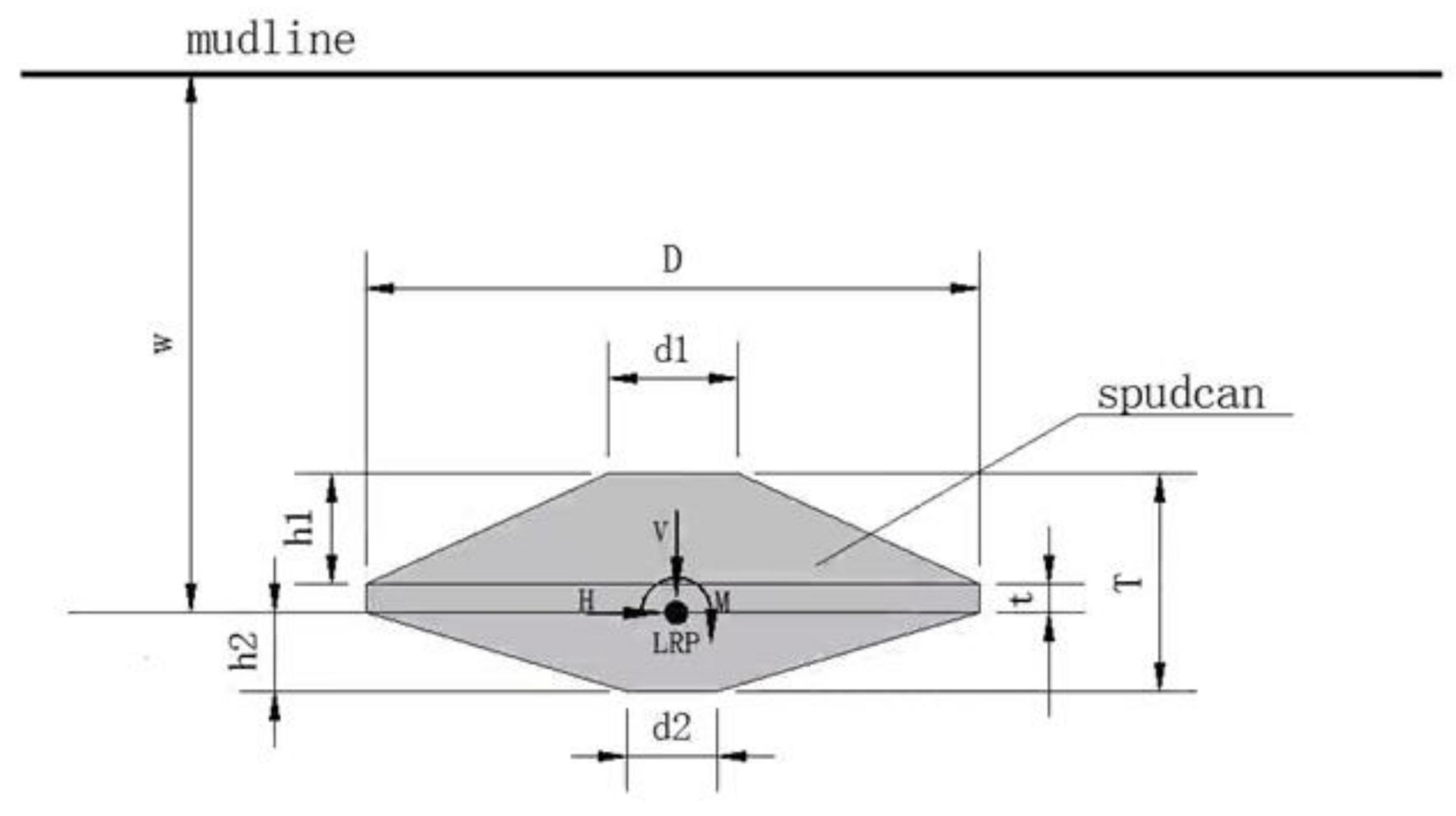
Figure 1.
Spudcan foundation and sign conventions for loads and displacements.
Figure 1.
Spudcan foundation and sign conventions for loads and displacements.
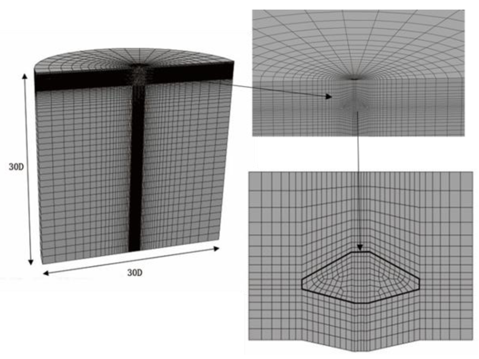
Figure 2.
Finite element model for a typical SSFE (small-strain finite element) computation (Spudcan-IV).
Figure 2.
Finite element model for a typical SSFE (small-strain finite element) computation (Spudcan-IV).
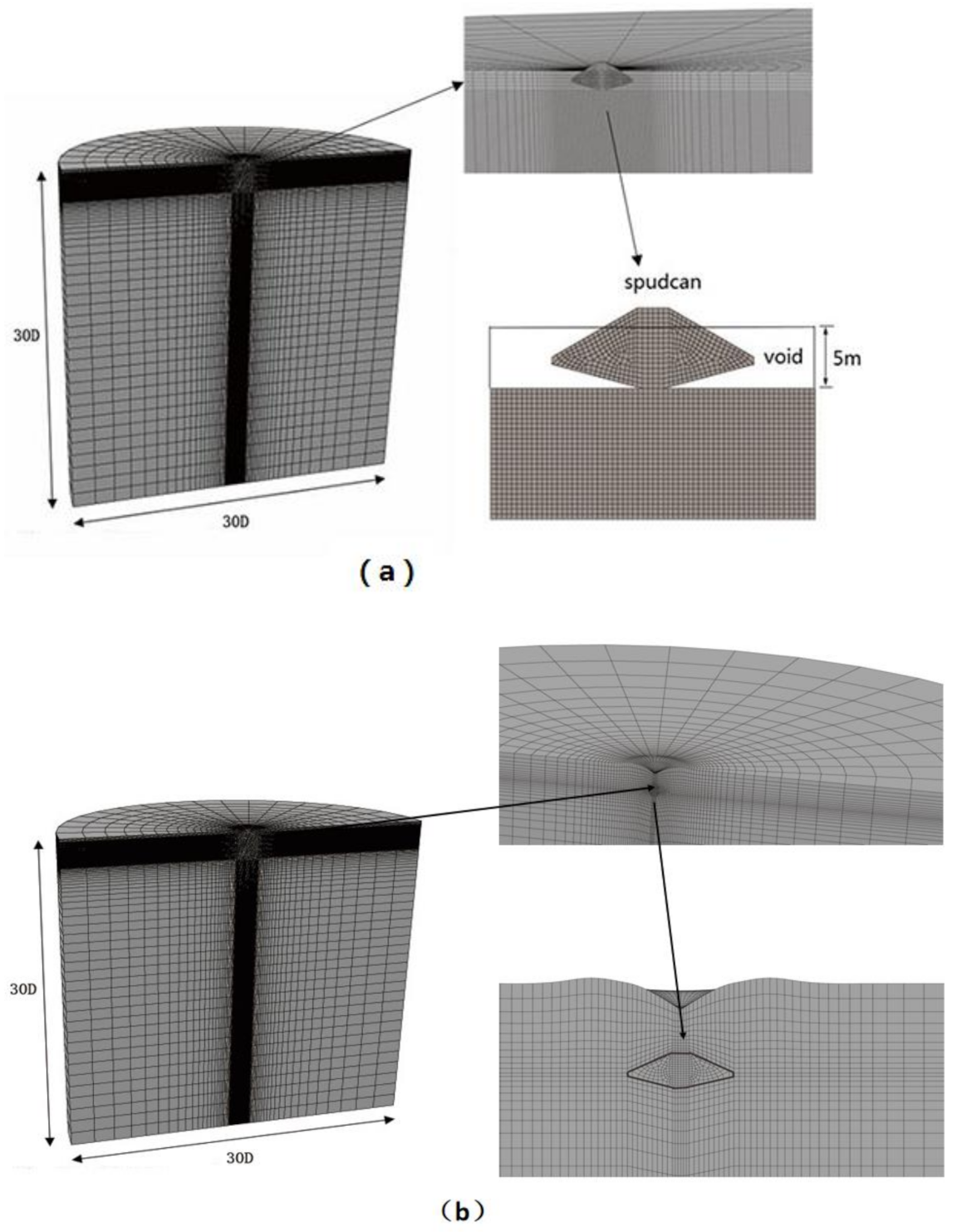
Figure 3.
Finite element model for a typical LDFE (large deformation finite element) computation with DSEL (dual-stage Eulerian–Lagrangian) technique (Spudcan-IV): (a) Eulerian finite element model, (b) Lagrangian finite element model.
Figure 3.
Finite element model for a typical LDFE (large deformation finite element) computation with DSEL (dual-stage Eulerian–Lagrangian) technique (Spudcan-IV): (a) Eulerian finite element model, (b) Lagrangian finite element model.
Figure 4.
Initial stress field of the small-strain Lagrangian analyses.
Figure 4.
Initial stress field of the small-strain Lagrangian analyses.
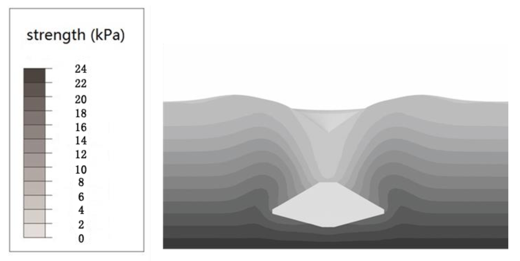
Figure 5.
Initial strength field of the small-strain Lagrangian analyses.
Figure 5.
Initial strength field of the small-strain Lagrangian analyses.
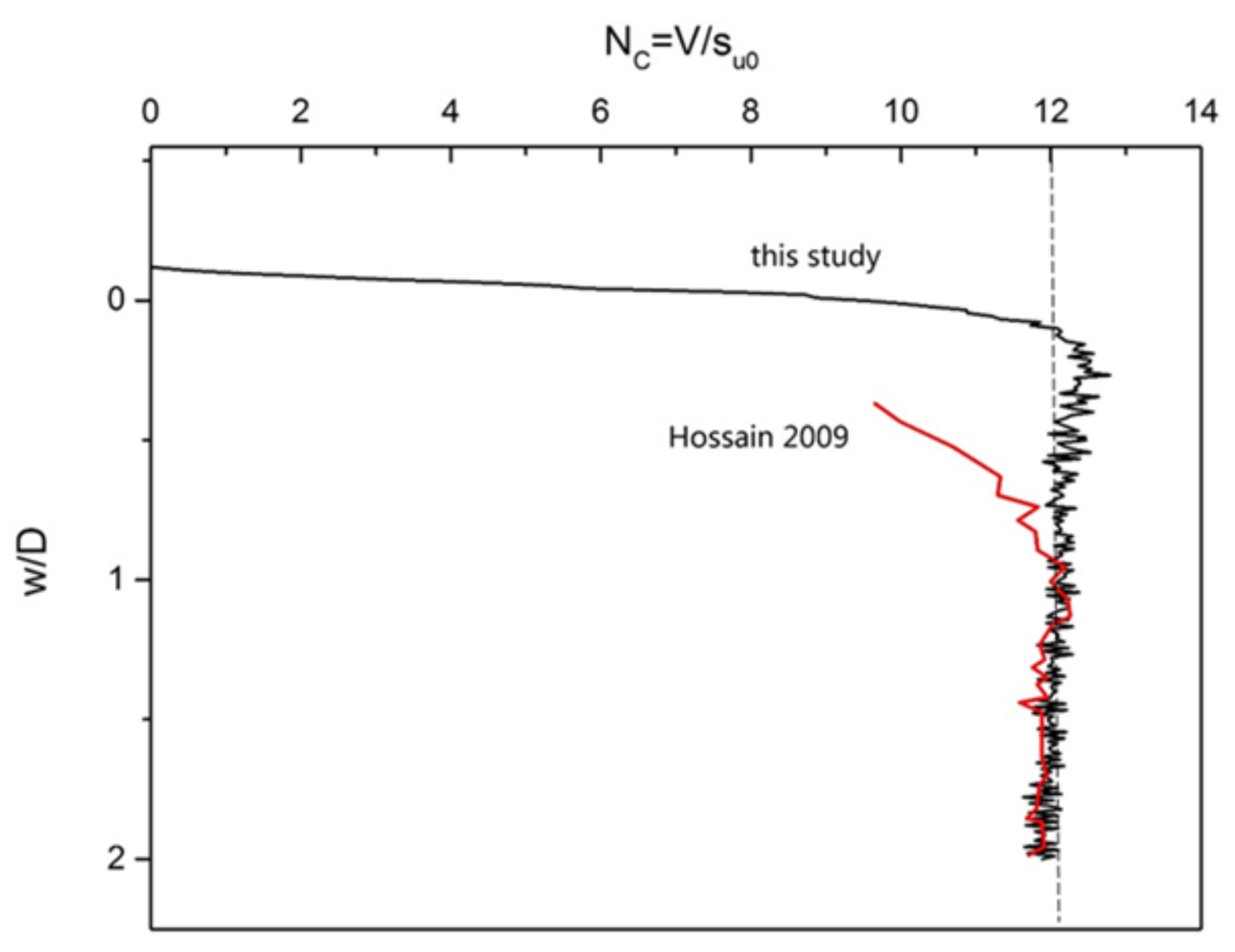
Figure 6.
Bearing capacity factor of a smooth spudcan inferred from LDFE calculation with DSEL technique. ( in the graph refers to the shear strength at the LRP (load reference point) elevation).
Figure 6.
Bearing capacity factor of a smooth spudcan inferred from LDFE calculation with DSEL technique. ( in the graph refers to the shear strength at the LRP (load reference point) elevation).
Figure 7.
Influence of and on when .
Figure 7.
Influence of and on when .
Figure 8.
Influence of and on when .
Figure 8.
Influence of and on when .
Figure 9.
Influence of and on when .
Figure 9.
Influence of and on when .
Figure 10.
Influence of and on when .
Figure 10.
Influence of and on when .
Figure 11.
Influence of and on when .
Figure 11.
Influence of and on when .
Figure 12.
Influence of and on when .
Figure 12.
Influence of and on when .
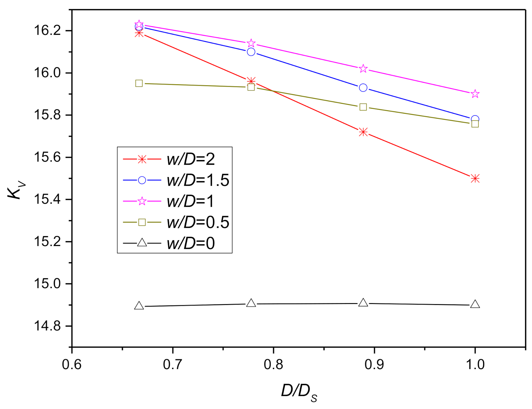
Figure 13.
Vertical dimensionless elastic stiffness coefficients with complete backflow of soil.
Figure 13.
Vertical dimensionless elastic stiffness coefficients with complete backflow of soil.
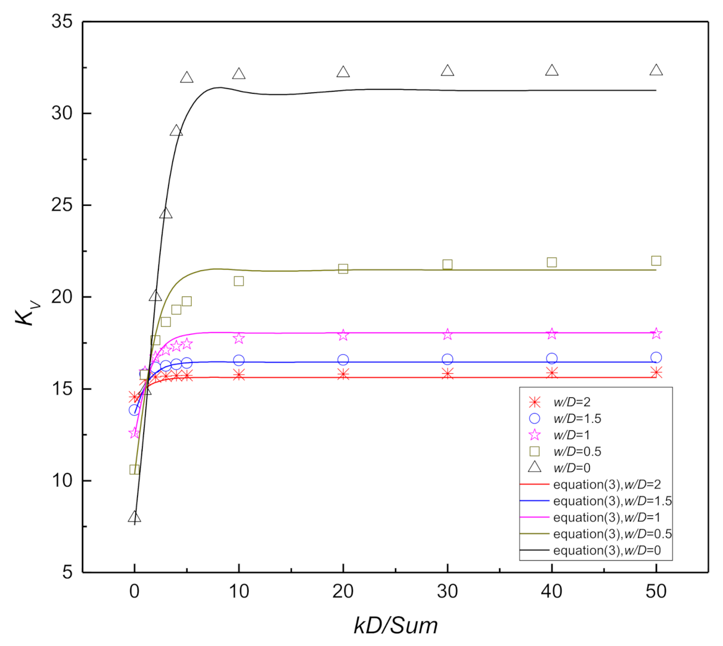
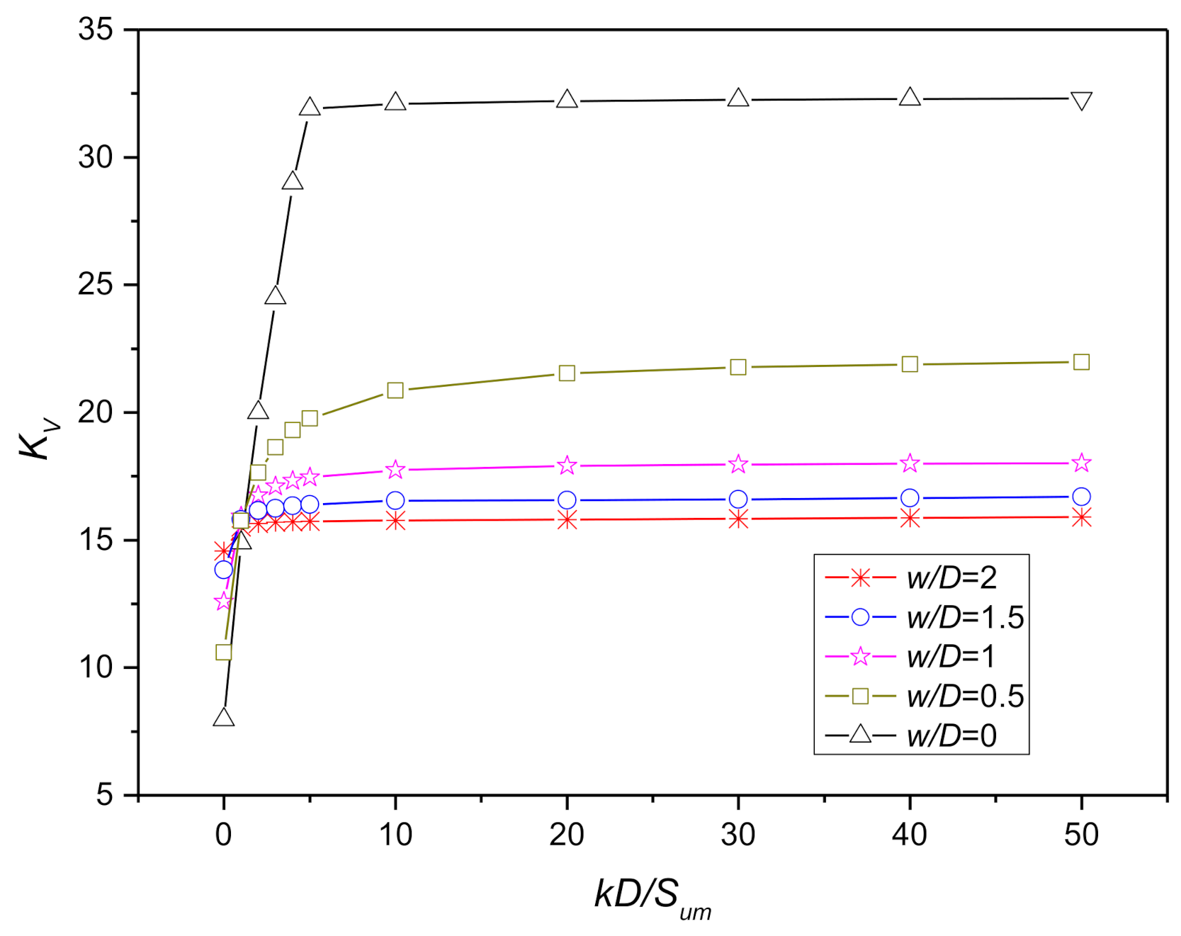
Figure 14.
Vertical dimensionless elastic stiffness coefficients with complete backflow of soil.
Figure 14.
Vertical dimensionless elastic stiffness coefficients with complete backflow of soil.
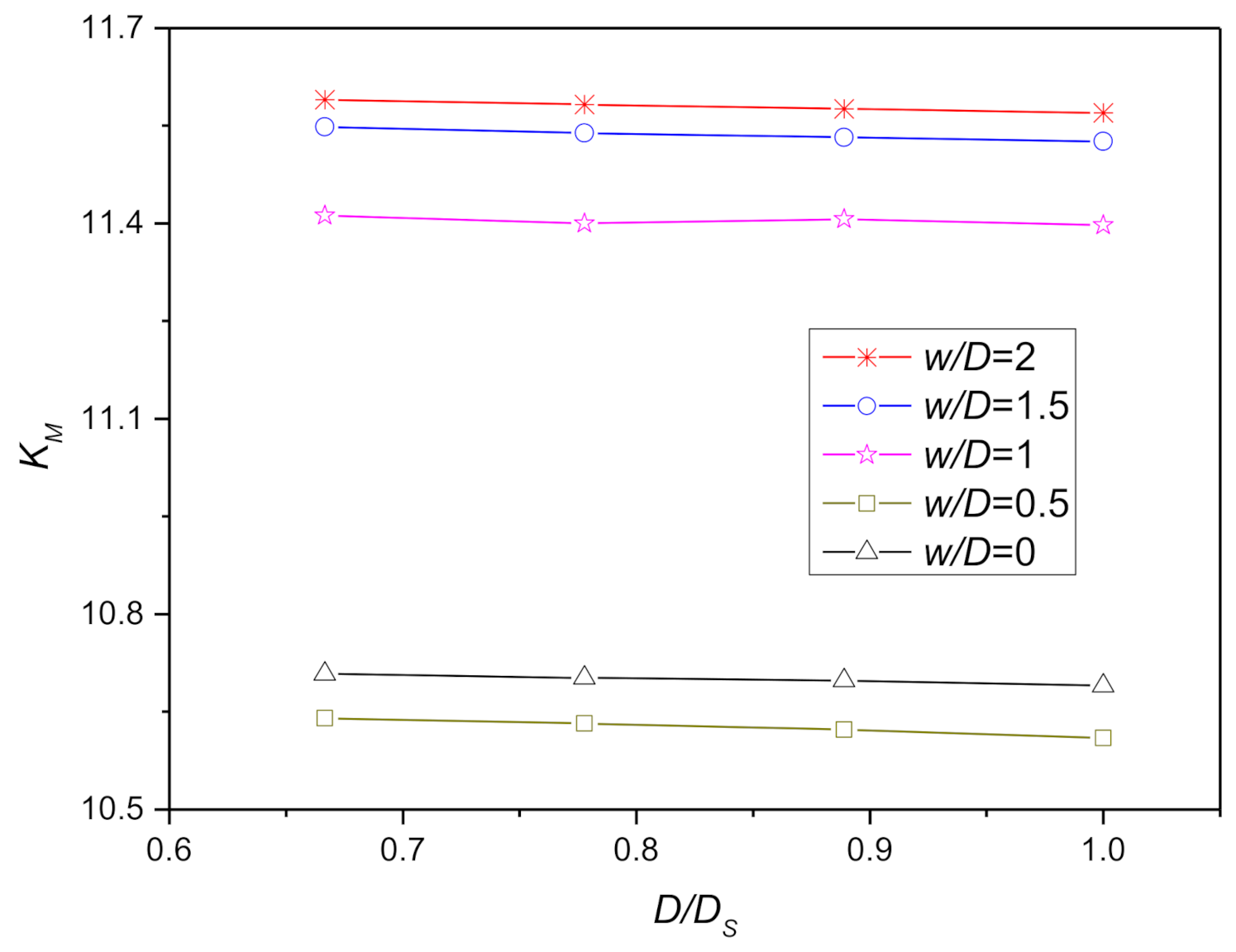
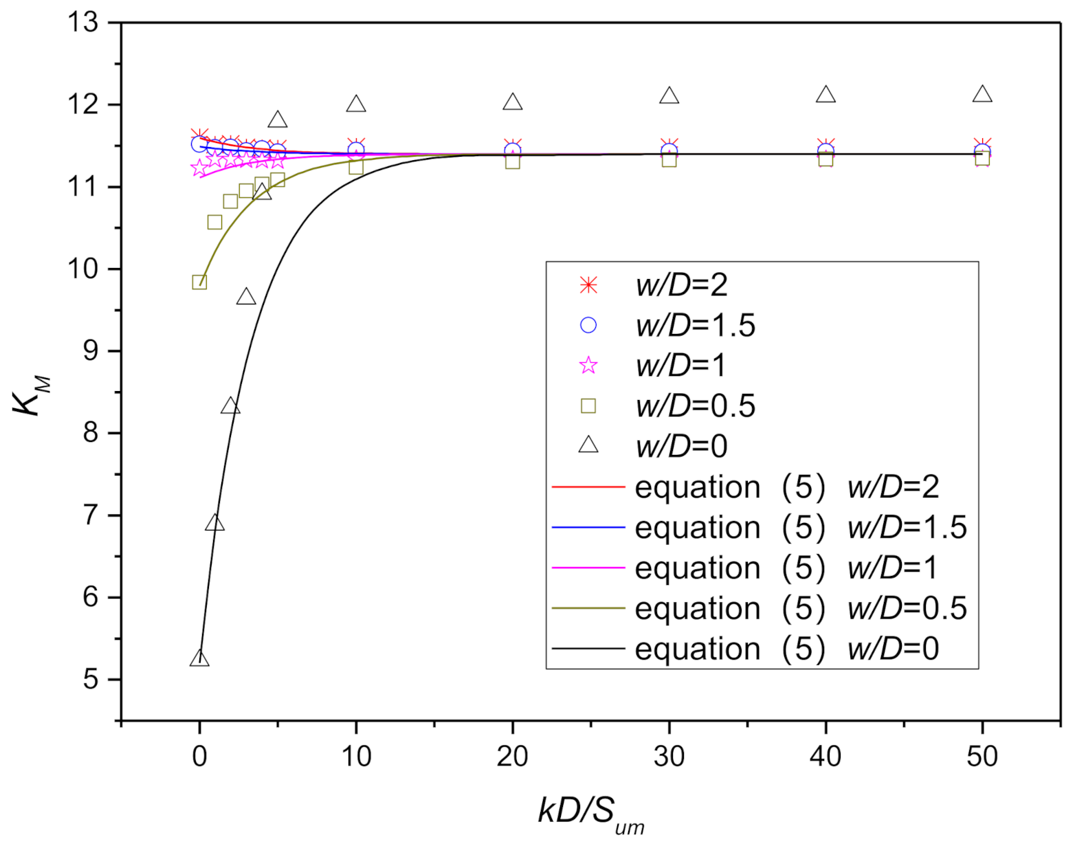
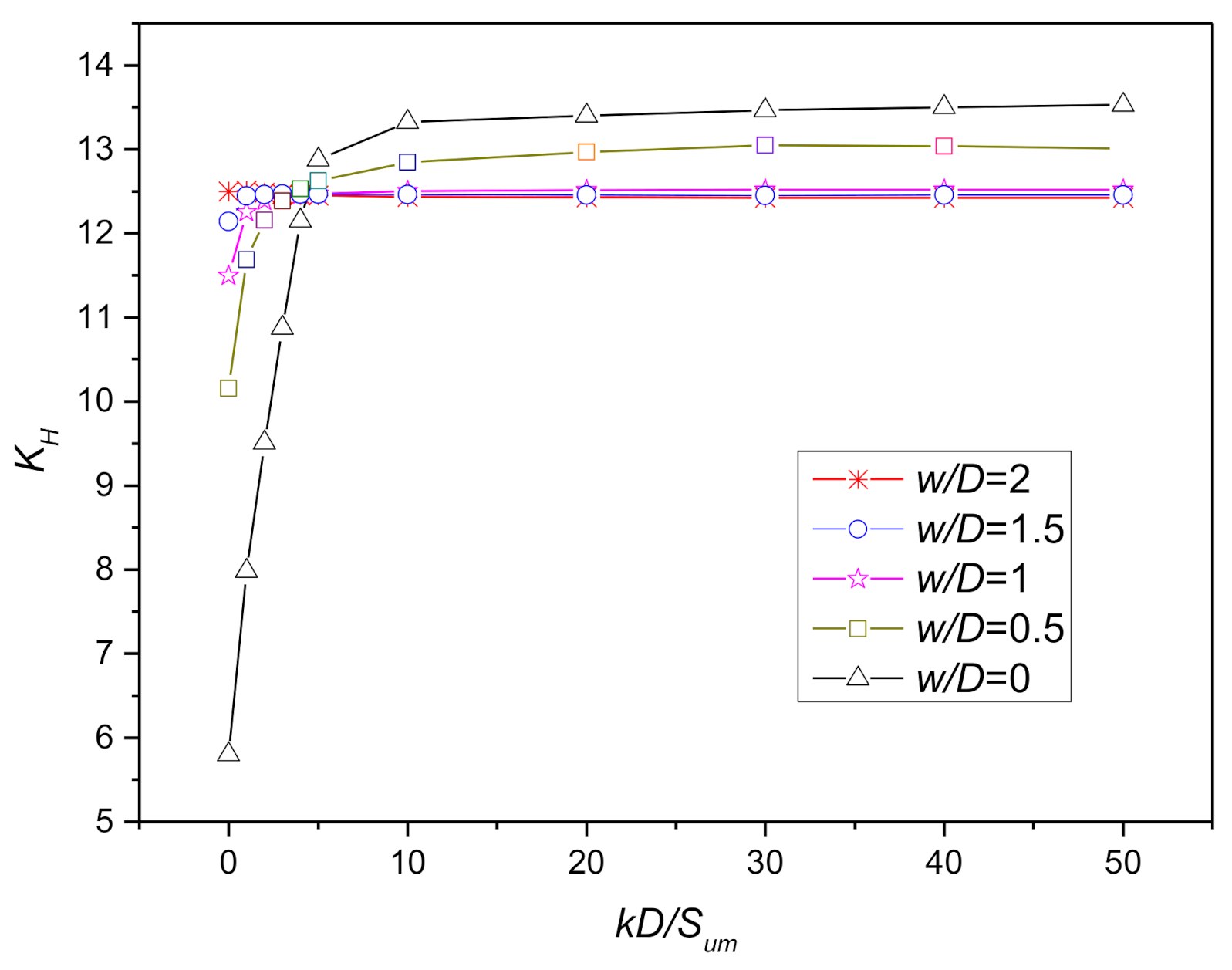
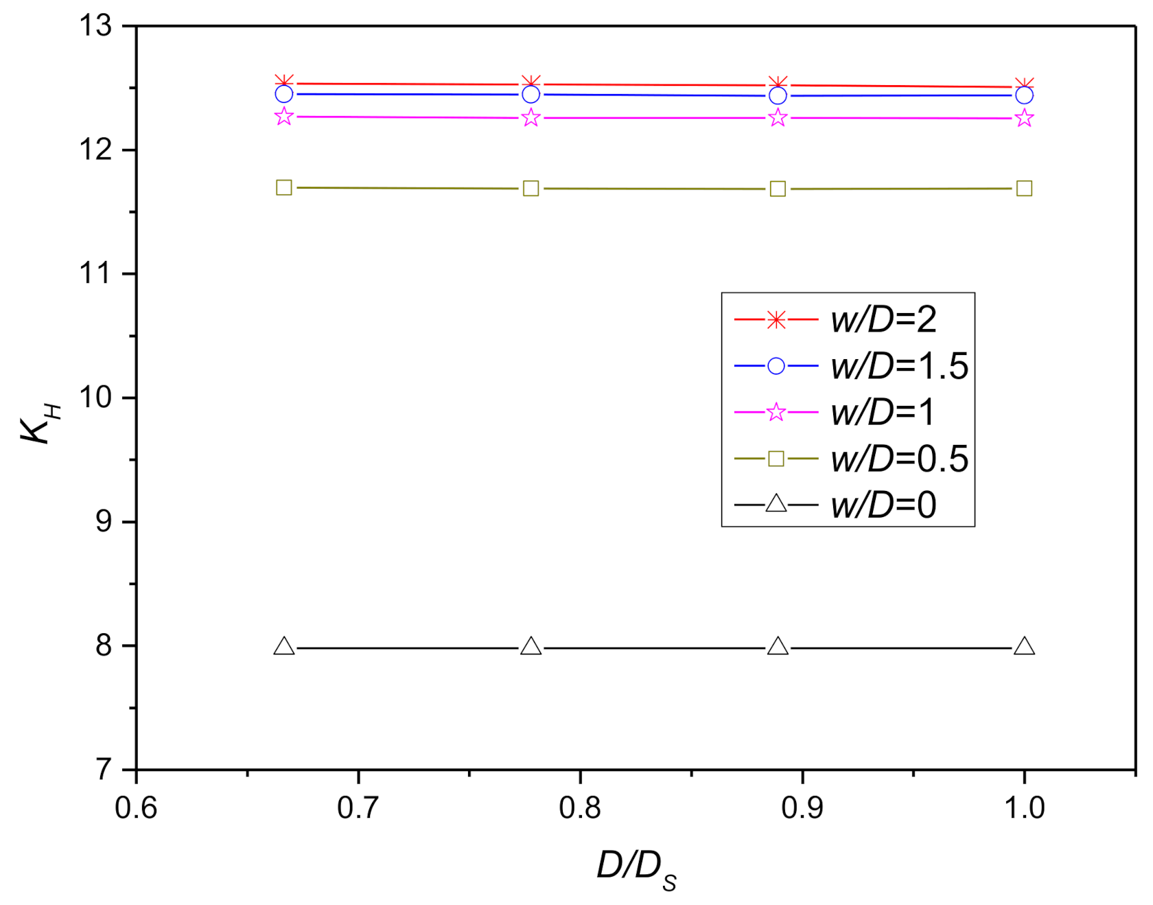
Figure 15.
Moment dimensionless elastic stiffness coefficients with complete backflow of soil.
Figure 15.
Moment dimensionless elastic stiffness coefficients with complete backflow of soil.
Figure 16.
Influence of and on when .
Figure 16.
Influence of and on when .
Figure 17.
Influence of on when .
Figure 17.
Influence of on when .
Figure 18.
Influence of on when .
Figure 18.
Influence of on when .
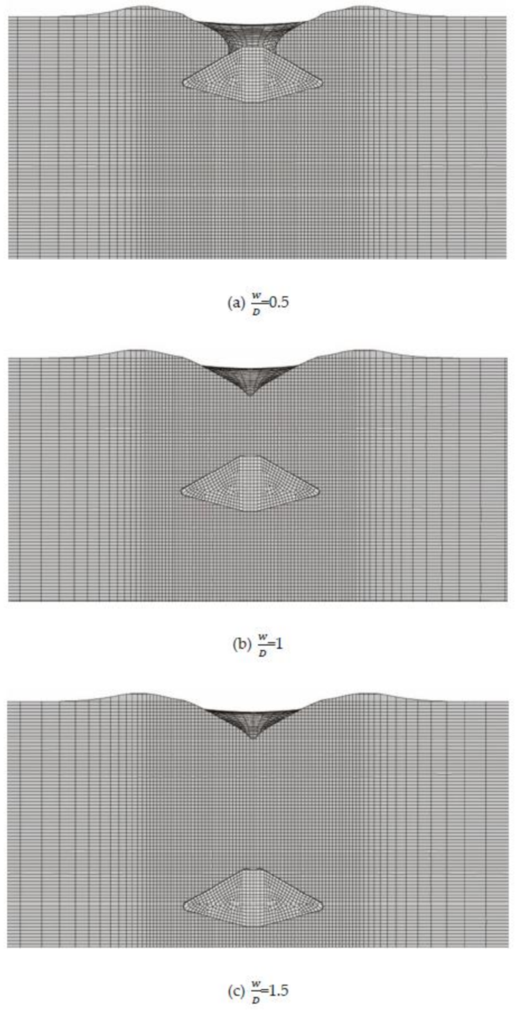
Figure 19.
Cavity at different penetration depths of the spudcan. (Spudcan-IV, , .
Figure 19.
Cavity at different penetration depths of the spudcan. (Spudcan-IV, , .
Figure 20.
Influence of on when .
Figure 20.
Influence of on when .
Figure 21.
Influence of when .
Figure 21.
Influence of when .
Figure 22.
Influence of on when
Figure 22.
Influence of on when
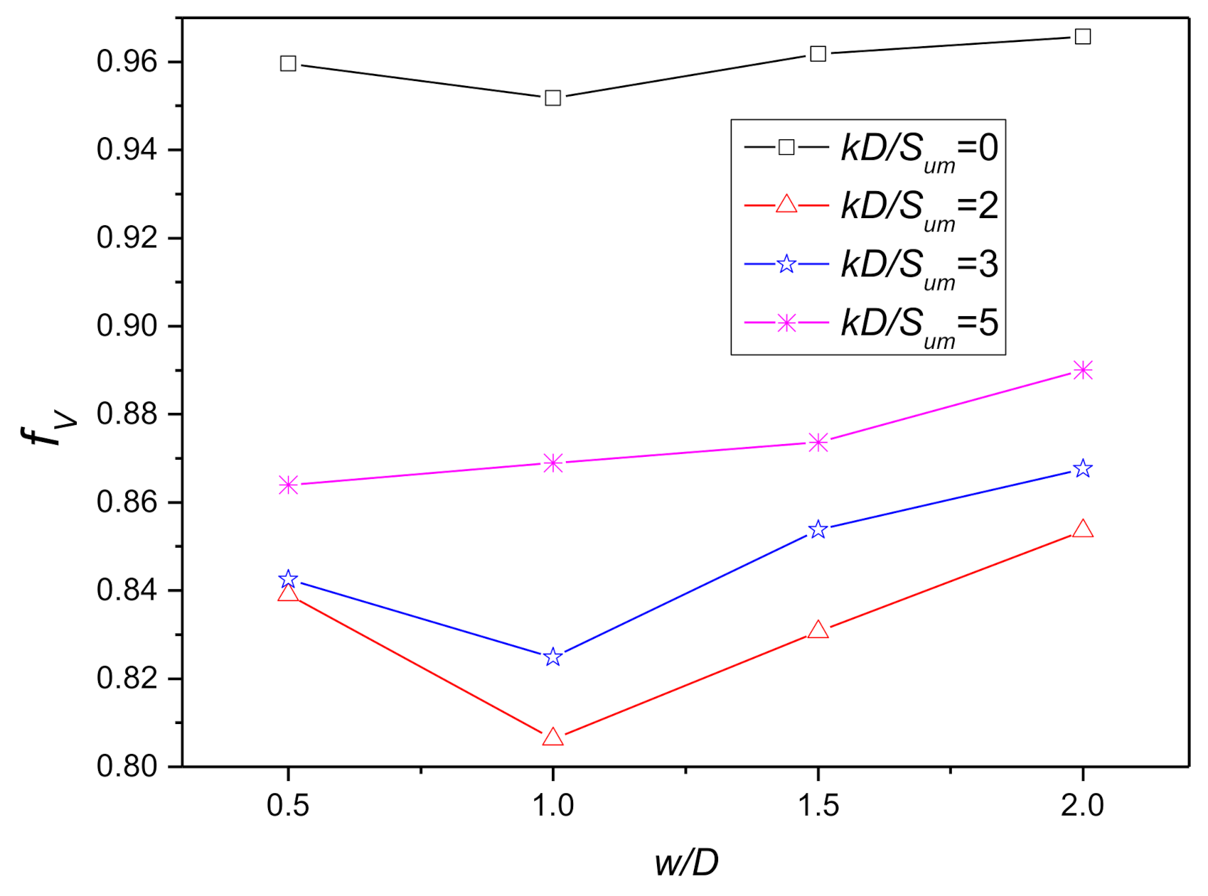
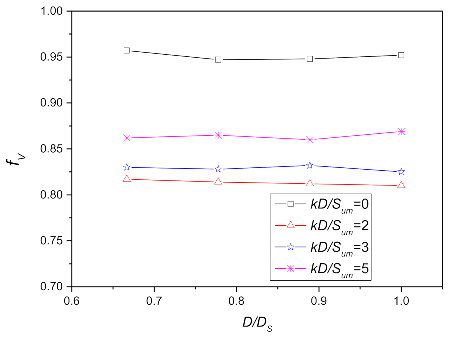
Figure 23.
Reduction factors of vertical dimensionless elastic stiffness coefficients related to and .
Figure 23.
Reduction factors of vertical dimensionless elastic stiffness coefficients related to and .
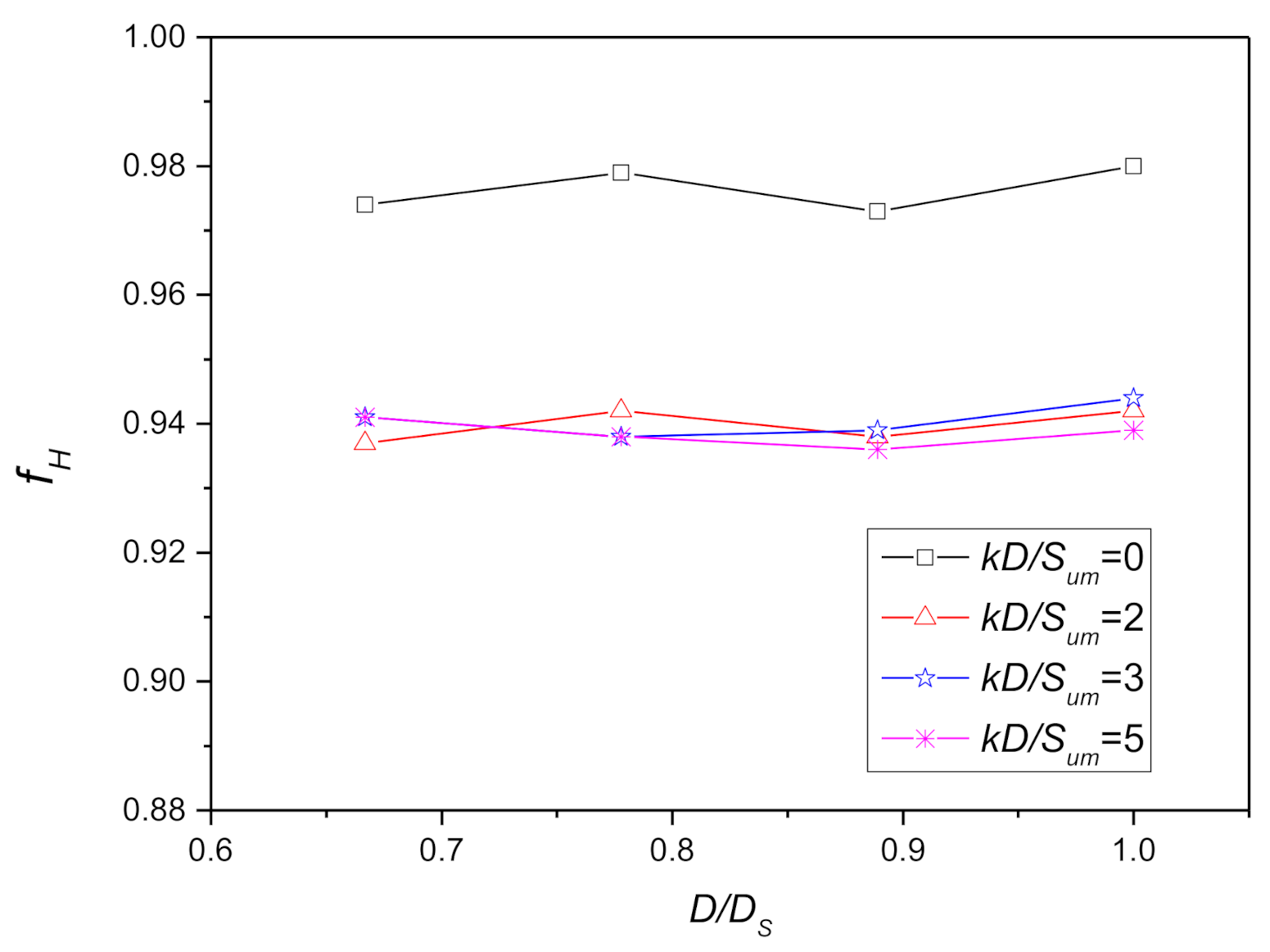
Figure 24.
Reduction factors of horizontal dimensionless elastic stiffness coefficients related to and .
Figure 24.
Reduction factors of horizontal dimensionless elastic stiffness coefficients related to and .
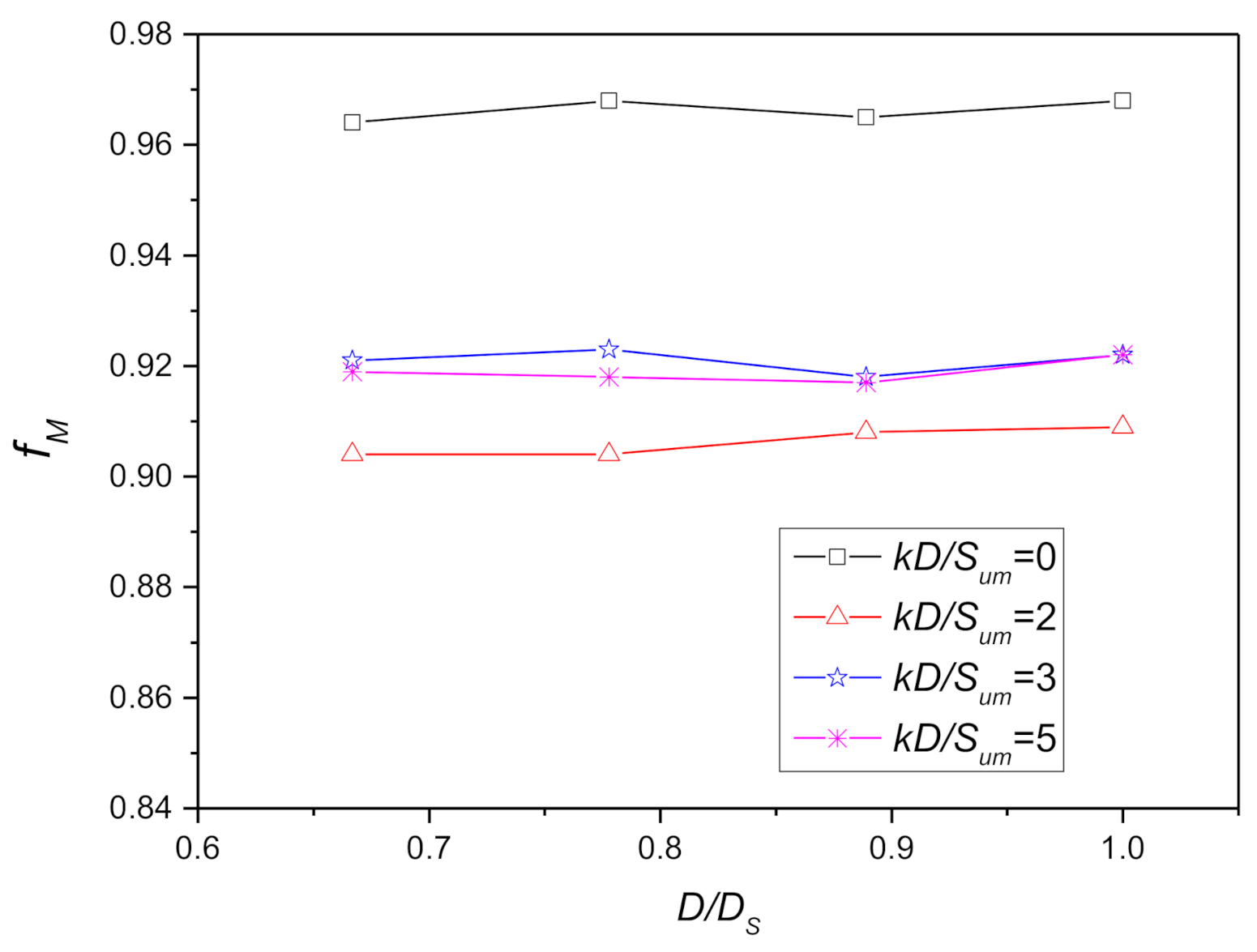
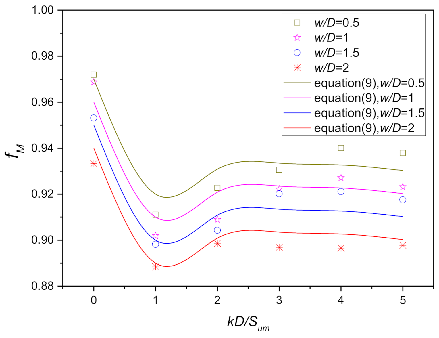
Figure 25.
Reduction factors of moment dimensionless elastic stiffness coefficients related to and .
Figure 25.
Reduction factors of moment dimensionless elastic stiffness coefficients related to and .
Table 1.
Dimensions of spudcans adopted in this study.
Table 1.
Dimensions of spudcans adopted in this study.
| ID | (m) | (m) | (m) | (m) | (m) | (m) |
|---|
| Spudcan-I | 12 | 2.43 | 0.37 | 1.20 | 1.57 | 1.04 |
| Spudcan-II | 14 | 2.92 | 0.44 | 1.44 | 1.88 | 1.25 |
| Spudcan-III | 16 | 3.41 | 0.51 | 1.68 | 2.19 | 1.46 |
| Spudcan-IV | 18 | 3.89 | 0.59 | 1.92 | 2.51 | 1.67 |
Table 2.
Validation of the finite element model with existing solutions.
Table 2.
Validation of the finite element model with existing solutions.
| | | | | |
|---|
| Rough Base | ISO19905-1 [12] | 7.843 | 5.299 | 5.229 |
| | Zhang [10] | 7.955 | 5.310 | 5.190 |
| | SSFE of this study | 7.924 | 5.312 | 5.194 |
| Smooth Base | Zhang [10] | 7.954 | | 5.189 |
| | Poulos and Davis [5] | 7.843 | | 5.229 |
| | SSFE of this study | 7.923 | | 5.192 |
Table 3.
Selection range of the parameter.
Table 3.
Selection range of the parameter.
| Factor | Unit | Selection Range |
|---|
| (strength gradient) | kPa/m | 0.2n, 0.25n, 0.28n, 0.3n
(n = 0, 1, 2, 3, 4, 5, 10, 20, 30, 40, 50) |
| (mudline shear strength) | kPa | 2.8, 3, 4.8, 5 |
| (embedded depth of the spudcan) | m | 6, 7, 8, 9, 12, 14, 16, 18, 21, 24, 27, 28, 32, 36 |
| (spudcan diameter) | m | 12, 14, 16, 18 |
Table 4.
Orthogonal experimental design.
Table 4.
Orthogonal experimental design.
| Test Number | (kPa/m) | (m) | (kPa) | (m) |
|---|
| Test 1 | 0.28 | 12 | 2.5 | 9 |
| Test 2 | 0.28 | 14 | 5 | 18 |
| Test 3 | 0.28 | 16 | 7.5 | 27 |
| Test 4 | 0.28 | 18 | 10 | 36 |
| Test 5 | 0.56 | 12 | 5 | 36 |
| Test 6 | 0.56 | 14 | 2.5 | 27 |
| Test 7 | 0.56 | 16 | 10 | 18 |
| Test 8 | 0.56 | 18 | 7.5 | 9 |
| Test 9 | 0.83 | 12 | 7.5 | 18 |
| Test 10 | 0.83 | 14 | 10 | 9 |
| Test 11 | 0.83 | 16 | 2.5 | 36 |
| Test 12 | 0.83 | 18 | 5 | 27 |
| Test 13 | 1.11 | 12 | 10 | 27 |
| Test 14 | 1.11 | 14 | 7.5 | 36 |
| Test 15 | 1.11 | 16 | 5 | 9 |
| Test 16 | 1.11 | 18 | 2.5 | 18 |
Table 5.
Comparison between the vertical stiffness coefficients from expressions and finite element analyses.
Table 5.
Comparison between the vertical stiffness coefficients from expressions and finite element analyses.
| Test Number | | | Difference (%) |
|---|
| Test 1 | 16.70 | 16.32 | −2.27 |
| Test 2 | 15.86 | 15.26 | −3.79 |
| Test 3 | 15.55 | 14.99 | −3.59 |
| Test 4 | 15.28 | 14.69 | −3.85 |
| Test 5 | 15.73 | 16.26 | 3.34 |
| Test 6 | 16.28 | 16.27 | −0.05 |
| Test 7 | 15.79 | 15.16 | −4.02 |
| Test 8 | 16.51 | 16.00 | −3.08 |
| Test 9 | 16.34 | 16.21 | −0.84 |
| Test 10 | 16.20 | 15.65 | −3.40 |
| Test 11 | 15.76 | 15.73 | −0.19 |
| Test 12 | 16.24 | 16.20 | −0.27 |
| Test 13 | 16.03 | 16.16 | 0.82 |
| Test 14 | 15.70 | 15.86 | 1.01 |
| Test 15 | 19.21 | 20.06 | 4.43 |
| Test 16 | 17.74 | 18.05 | 1.72 |
Table 6.
Comparison between the horizontal stiffness coefficients from expressions and finite element analyses.
Table 6.
Comparison between the horizontal stiffness coefficients from expressions and finite element analyses.
| Test Number | | | Difference (%) |
|---|
| Test 1 | 12.20 | 12.04 | −1.32 |
| Test 2 | 12.34 | 12.30 | −0.32 |
| Test 3 | 12.45 | 12.50 | 0.43 |
| Test 4 | 12.51 | 12.66 | 1.17 |
| Test 5 | 12.58 | 12.91 | 2.59 |
| Test 6 | 12.51 | 12.52 | 0.09 |
| Test 7 | 12.28 | 12.25 | −0.29 |
| Test 8 | 11.89 | 11.85 | −0.27 |
| Test 9 | 12.46 | 12.41 | −0.47 |
| Test 10 | 12.00 | 11.91 | −0.74 |
| Test 11 | 12.48 | 12.54 | 0.52 |
| Test 12 | 12.46 | 12.41 | −0.44 |
| Test 13 | 12.55 | 12.68 | 1.07 |
| Test 14 | 12.53 | 12.72 | 1.59 |
| Test 15 | 12.48 | 12.37 | −0.93 |
| Test 16 | 12.52 | 12.41 | −0.89 |
Table 7.
Comparison between the moment stiffness coefficients from expressions and finite element analyses.
Table 7.
Comparison between the moment stiffness coefficients from expressions and finite element analyses.
| Test Number | | | Difference (%) |
|---|
| Test 1 | 11.22 | 11.00 | −1.96 |
| Test 2 | 11.49 | 11.37 | −1.07 |
| Test 3 | 11.56 | 11.42 | −1.17 |
| Test 4 | 11.57 | 11.43 | −1.18 |
| Test 5 | 11.60 | 11.44 | −1.42 |
| Test 6 | 11.52 | 11.47 | −0.42 |
| Test 7 | 11.44 | 11.31 | −1.11 |
| Test 8 | 10.72 | 10.52 | −1.86 |
| Test 9 | 11.52 | 11.43 | −0.80 |
| Test 10 | 11.02 | 10.80 | −2.03 |
| Test 11 | 11.53 | 11.47 | −0.52 |
| Test 12 | 11.44 | 11.46 | 0.22 |
| Test 13 | 11.58 | 11.45 | −1.15 |
| Test 14 | 11.57 | 11.45 | −1.03 |
| Test 15 | 11.13 | 10.89 | −2.20 |
| Test 16 | 11.38 | 11.40 | 0.20 |
Table 8.
Comparison between the vertical stiffness coefficients of a spudcan embedded in pure elastic and elastic perfectly plastic soil.
Table 8.
Comparison between the vertical stiffness coefficients of a spudcan embedded in pure elastic and elastic perfectly plastic soil.
| KD/Sum | W/D | | | Difference (%) |
|---|
| 0 | 1 | 12.492 | 12.587 | 0.757 |
| 1 | 1 | 15.837 | 15.925 | 0.554 |
| 2 | 1 | 16.682 | 16.739 | 0.342 |
| 3 | 1 | 17.188 | 17.099 | −0.520 |
| 4 | 1 | 17.275 | 17.313 | 0.217 |
| 5 | 1 | 17.465 | 17.450 | −0.086 |
| 4 | 0.5 | 19.272 | 19.306 | 0.176 |
| 4 | 1.5 | 16.190 | 16.340 | 0.928 |
| 4 | 2 | 15.887 | 15.724 | −1.027 |
Table 9.
Comparison between the horizontal stiffness coefficients of a spudcan embedded in pure elastic and elastic perfectly plastic soil.
Table 9.
Comparison between the horizontal stiffness coefficients of a spudcan embedded in pure elastic and elastic perfectly plastic soil.
| KD/Sum | W/D | | | Difference (%) |
|---|
| 0 | 1 | 11.457 | 11.497 | 0.349 |
| 1 | 1 | 12.335 | 12.255 | −0.649 |
| 2 | 1 | 12.347 | 12.385 | 0.308 |
| 3 | 1 | 12.429 | 12.433 | 0.032 |
| 4 | 1 | 12.451 | 12.459 | 0.066 |
| 5 | 1 | 12.466 | 12.474 | 0.064 |
| 4 | 0.5 | 12.557 | 12.532 | −0.199 |
| 4 | 1.5 | 12.459 | 12.465 | 0.048 |
| 4 | 2 | 12.453 | 12.457 | 0.032 |
Table 10.
Comparison between the moment initial stiffness coefficients of a spudcan embedded in pure elastic and elastic perfectly plastic soil.
Table 10.
Comparison between the moment initial stiffness coefficients of a spudcan embedded in pure elastic and elastic perfectly plastic soil.
| KD/Sum | W/D | | | Difference (%) |
|---|
| 0 | 1 | 11.221 | 11.226 | 0.045 |
| 1 | 1 | 11.339 | 11.333 | −0.053 |
| 2 | 1 | 11.345 | 11.333 | −0.106 |
| 3 | 1 | 11.342 | 11.327 | −0.132 |
| 4 | 1 | 11.351 | 11.321 | −0.263 |
| 5 | 1 | 11.323 | 11.317 | −0.053 |
| 4 | 0.5 | 11.029 | 11.031 | 0.018 |
| 4 | 1.5 | 11.482 | 11.460 | −0.192 |
| 4 | 2 | 11.530 | 11.471 | −0.511 |
Table 11.
Comparison between the reduction factors of vertical stiffness from fitted expressions and finite element analyses.
Table 11.
Comparison between the reduction factors of vertical stiffness from fitted expressions and finite element analyses.
| Test Number | | | Difference (%) |
|---|
| Test 1 | 0.889 | 0.913 | 2.69 |
| Test 2 | 0.914 | 0.925 | 1.18 |
| Test 3 | 0.968 | 0.931 | −3.74 |
| Test 4 | 0.912 | 0.935 | 2.58 |
| Test 5 | 0.918 | 0.911 | −0.81 |
| Test 6 | 0.973 | 0.939 | −3.55 |
| Test 7 | 0.914 | 0.921 | 0.77 |
| Test 8 | 0.934 | 0.913 | −2.21 |
| Test 9 | 0.898 | 0.912 | 1.62 |
| Test 10 | 0.893 | 0.916 | 2.52 |
| Test 11 | 0.986 | 0.949 | −3.78 |
| Test 12 | 0.879 | 0.934 | 6.36 |
| Test 13 | 0.860 | 0.911 | 6.00 |
| Test 14 | 0.888 | 0.914 | 2.89 |
| Test 15 | 0.896 | 0.951 | 6.11 |
| Test 16 | 0.907 | 0.958 | 5.64 |
Table 12.
Comparison between the reduction factors of horizontal stiffness from fitted expressions and finite element analyses.
Table 12.
Comparison between the reduction factors of horizontal stiffness from fitted expressions and finite element analyses.
| Test Number | | | Difference (%) |
|---|
| Test 1 | 0.935 | 0.942 | 0.71 |
| Test 2 | 0.944 | 0.935 | −1.05 |
| Test 3 | 0.973 | 0.930 | −4.42 |
| Test 4 | 0.938 | 0.927 | −1.22 |
| Test 5 | 0.937 | 0.912 | −2.69 |
| Test 6 | 0.883 | 0.917 | 3.79 |
| Test 7 | 0.958 | 0.937 | −2.19 |
| Test 8 | 0.914 | 0.948 | 3.69 |
| Test 9 | 0.913 | 0.930 | 1.82 |
| Test 10 | 0.936 | 0.945 | 0.90 |
| Test 11 | 0.949 | 0.905 | −4.69 |
| Test 12 | 0.906 | 0.924 | 1.90 |
| Test 13 | 0.937 | 0.920 | −1.78 |
| Test 14 | 0.947 | 0.913 | −3.58 |
| Test 15 | 0.931 | 0.940 | 1.02 |
| Test 16 | 0.907 | 0.920 | 1.34 |
Table 13.
Comparison between the reduction factors of moment stiffness from fitted expressions and finite element analyses.
Table 13.
Comparison between the reduction factors of moment stiffness from fitted expressions and finite element analyses.
| Test Number | | | Difference (%) |
|---|
| Test 1 | 0.877 | 0.920 | 4.97 |
| Test 2 | 0.886 | 0.900 | 1.55 |
| Test 3 | 0.910 | 0.887 | −2.58 |
| Test 4 | 0.846 | 0.878 | 3.78 |
| Test 5 | 0.878 | 0.875 | −0.30 |
| Test 6 | 0.860 | 0.905 | 5.24 |
| Test 7 | 0.871 | 0.905 | 4.00 |
| Test 8 | 0.904 | 0.925 | 2.29 |
| Test 9 | 0.895 | 0.905 | 1.13 |
| Test 10 | 0.873 | 0.920 | 5.33 |
| Test 11 | 0.880 | 0.894 | 1.66 |
| Test 12 | 0.882 | 0.913 | 3.61 |
| Test 13 | 0.866 | 0.890 | 2.76 |
| Test 14 | 0.882 | 0.890 | 0.92 |
| Test 15 | 0.910 | 0.932 | 2.39 |
| Test 16 | 0.897 | 0.910 | 1.46 |
Table 14.
Effect of spudcan installation on dimensionless initial stiffness coefficients.
Table 14.
Effect of spudcan installation on dimensionless initial stiffness coefficients.
| | | | |
|---|
| Stiffness coefficients with consideration of installation effect (Equations (3)–(5)) | 15.86 | 12.72 | 11.45 |
| Stiffness coefficients with consideration of installation effect (Equations (6)–(8)) | 14.49 | 11.62 | 10.19 |
| Difference (%) | −8.65 | −8.7 | −11.45 |


