
The Importance of Geotechnical Evaluation and Shoreline Evolution in Coastal Vulnerability Index Calculations


 ,
,  and
and 
Abstract
1. Introduction
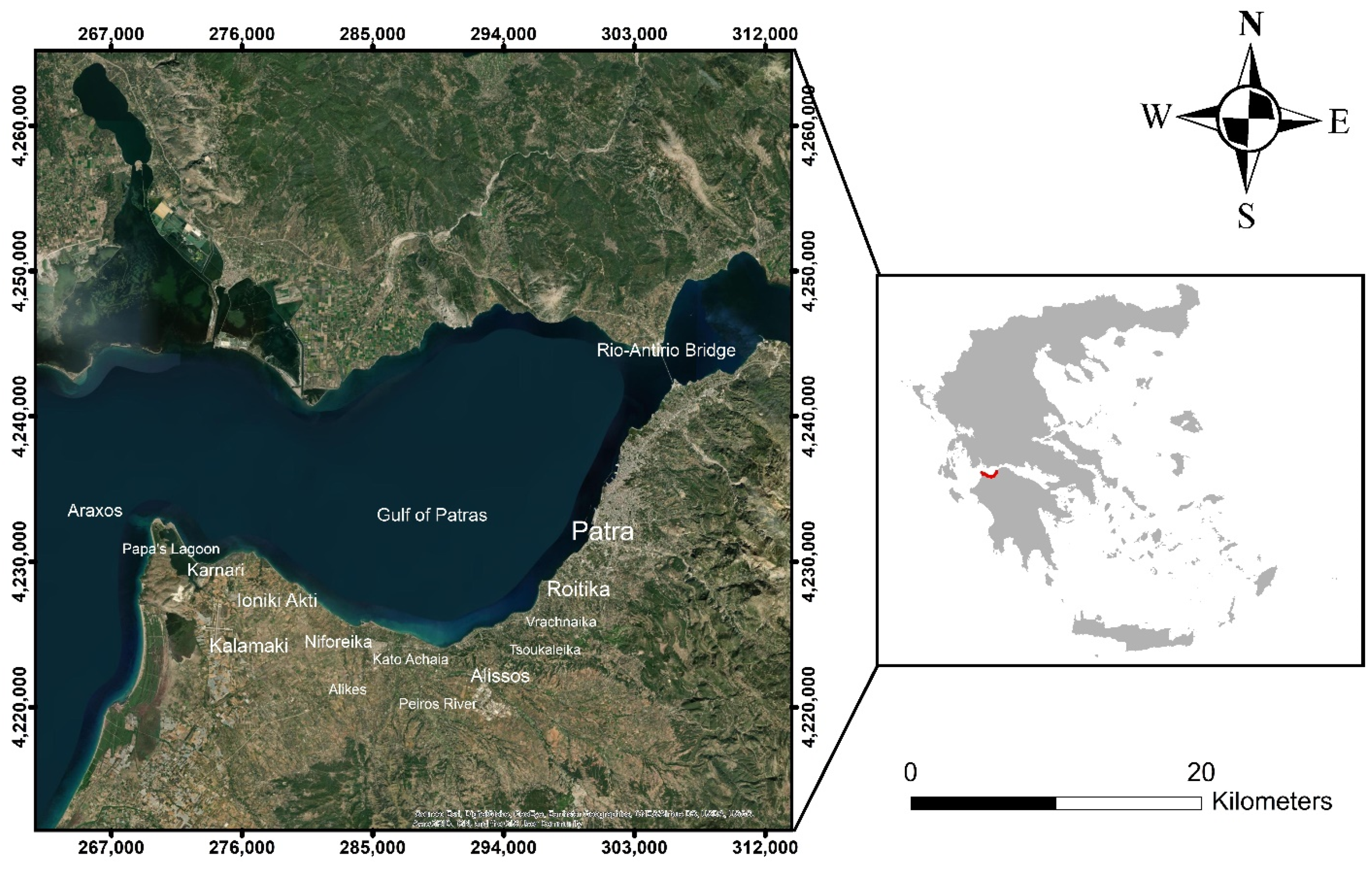
2. Study Area
3. Materials and Methods
3.1. Geotechnical Characterization
3.2. Significant Mean Wave Height
3.3. Coastal Slope
3.4. Shoreline Evolution
3.5. Average Tidal Range
3.6. Sea Level Rise (SLR)
3.7. CVI Calculation and Ranking
4. Results
4.1. Geotechnical Characterization
4.2. Significant Mean Wave Height
4.3. Coastal Slope
4.4. Shoreline Evolution
4.5. Average Tidal Range and SLR
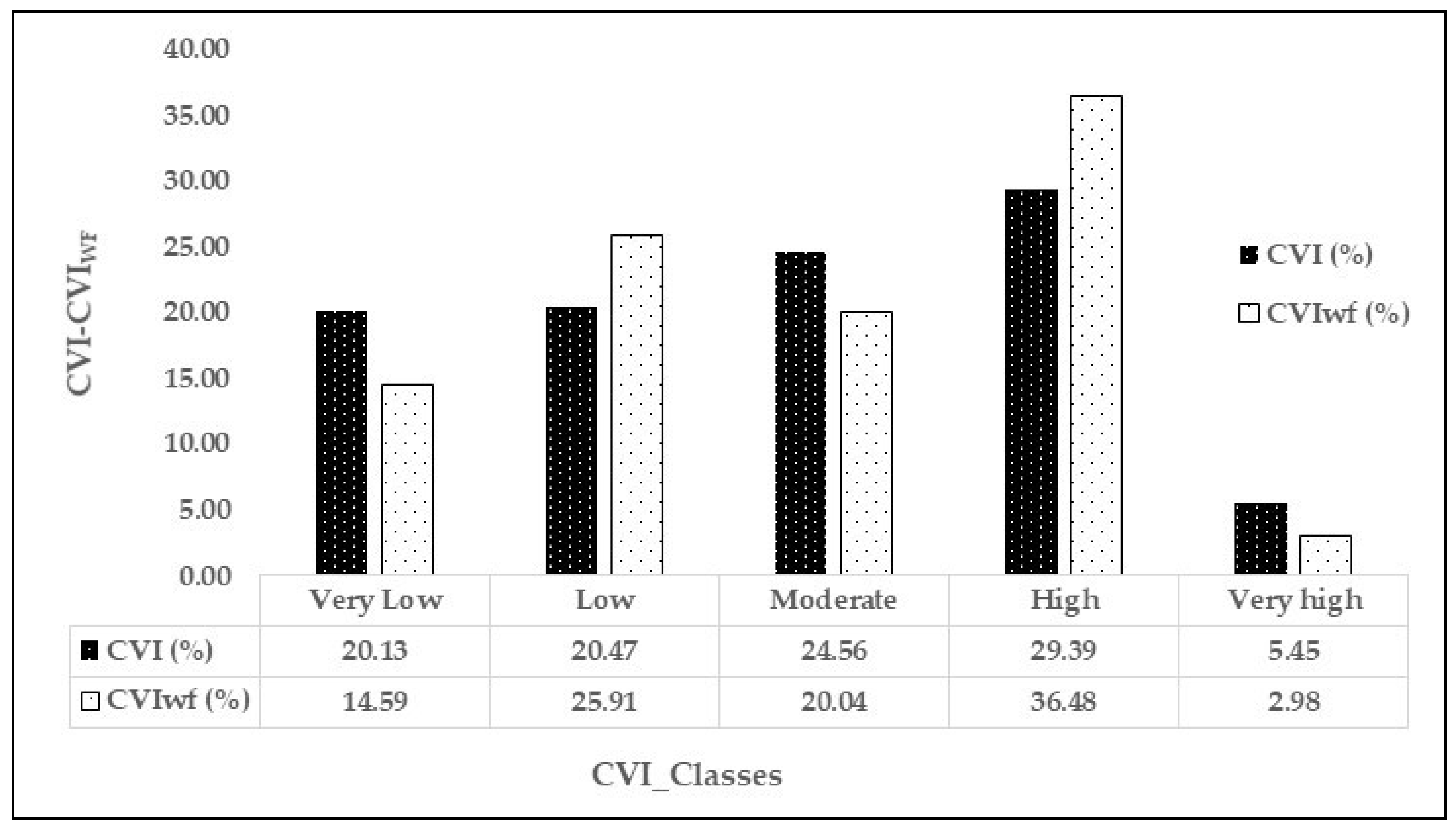
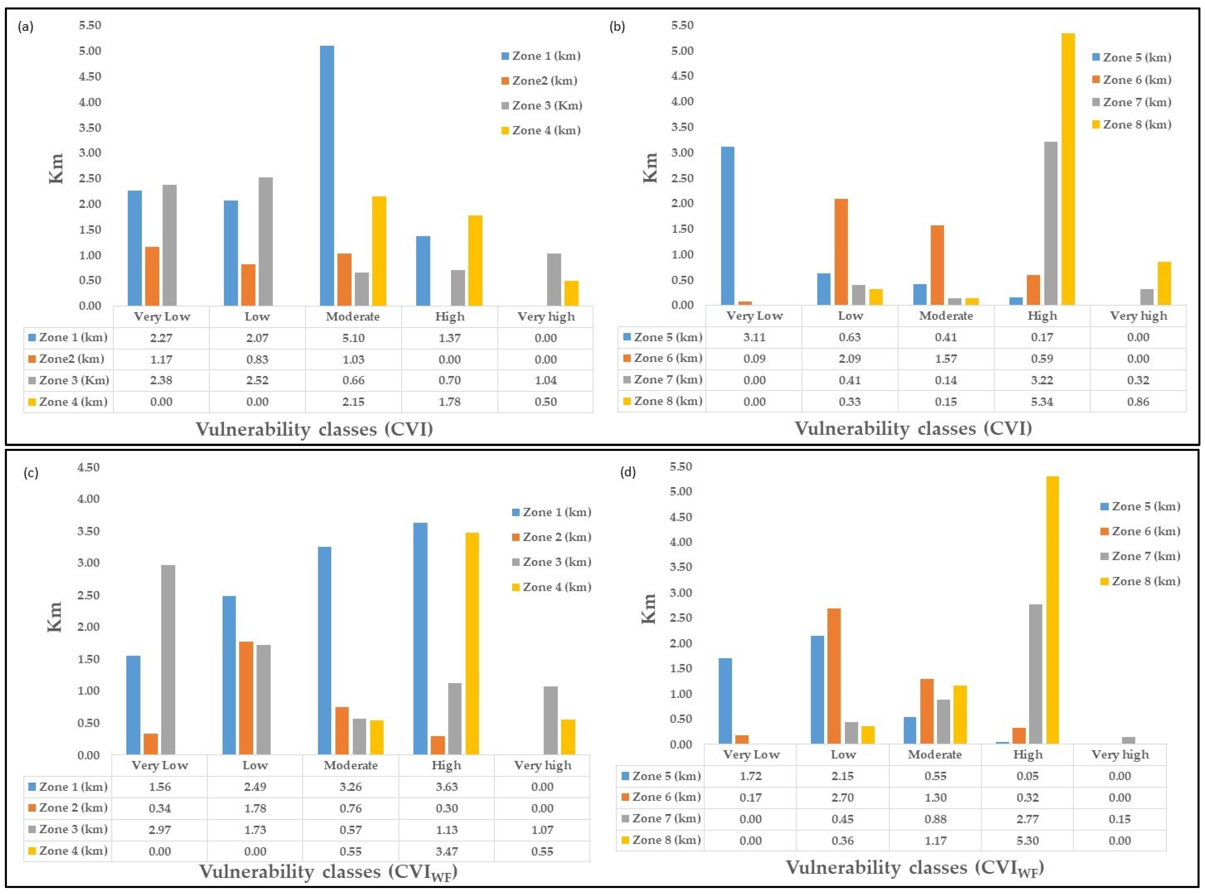
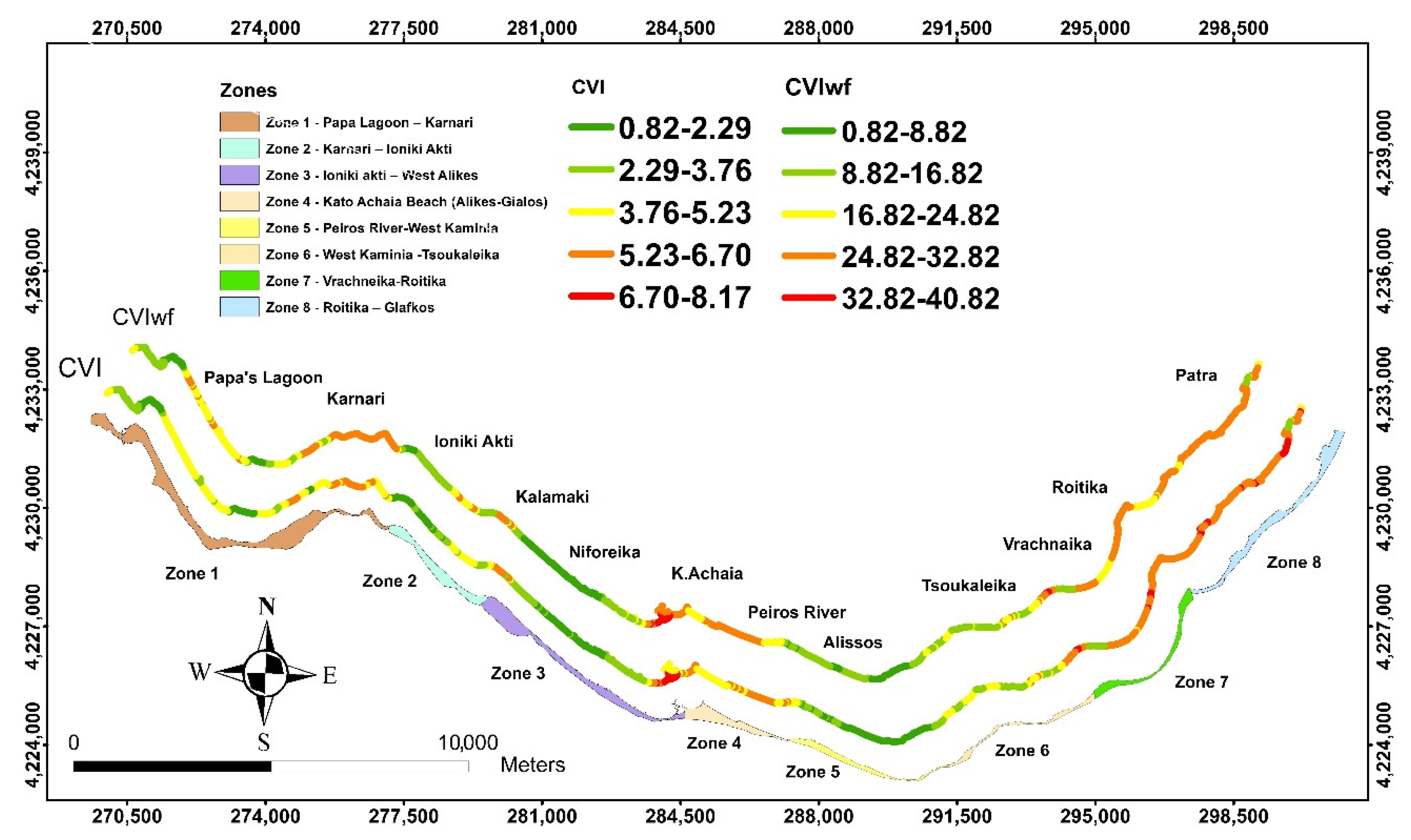
4.6. Comparison between the CVI and CVIWF Results
4.7. Analysis on the Weighted Geotechnical Factor Applied on CVIWF Equation
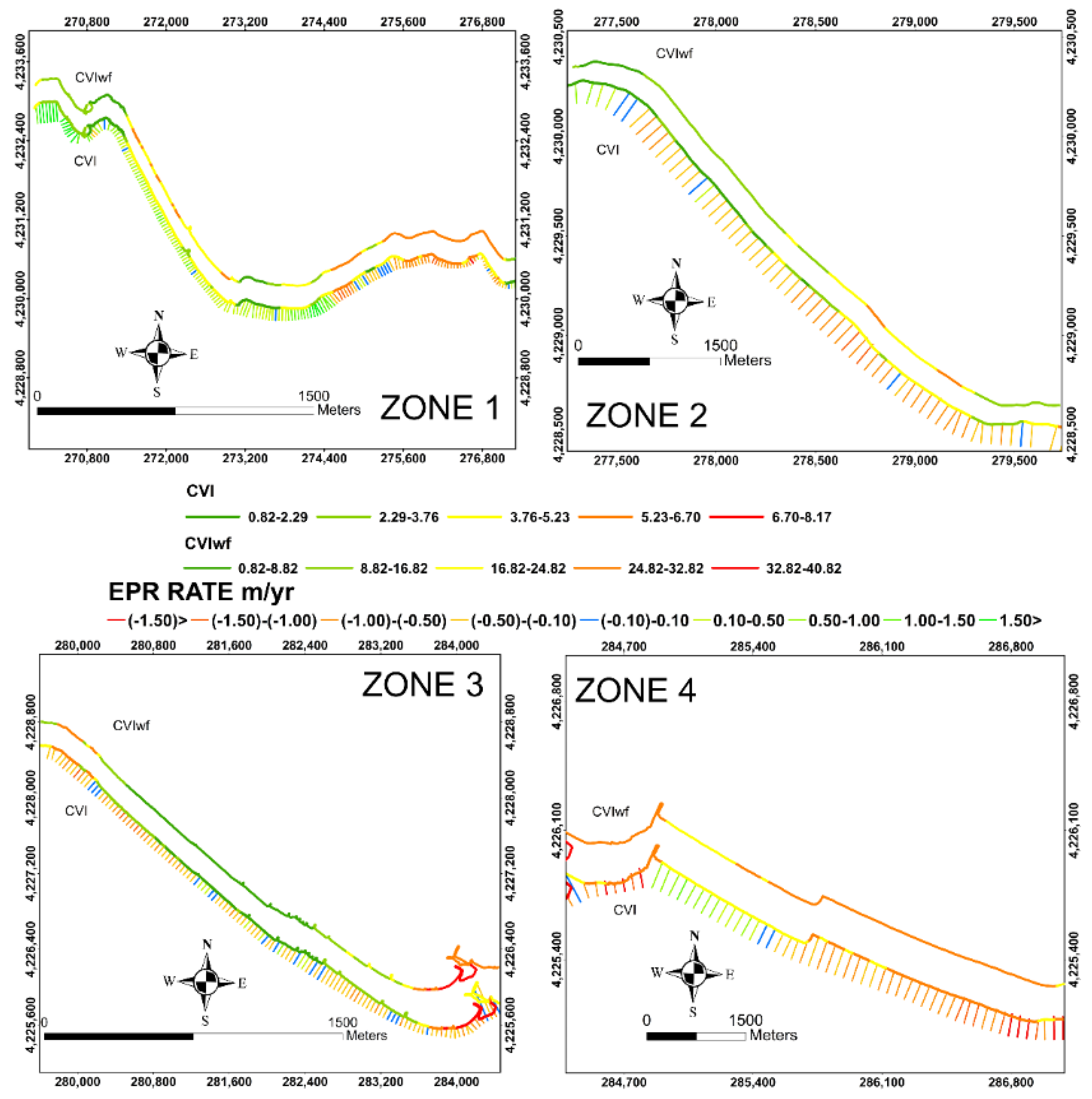
4.8. Analysis on the Computed EPR Values and the Respective CVIWF Results
5. Discussion
6. Conclusions
Author Contributions
Funding
Institutional Review Board Statement
Informed Consent Statement
Data Availability Statement
Acknowledgments

Conflicts of Interest
References
- IPCC. Global Warming of 1.5°C. Available online: https://www.ipcc.ch/sr15/ (accessed on 30 September 2020).
- EUROSION. Living with Coastal Erosion in Europe: Sediment and Space for Sustainability; European Environment Agency: Copenhagen, Denmark, 2004. [Google Scholar]
- Ramieri, E.; Hartley, A.; Barbanti, A.; Duarte Santos, F.; Gomes, A.; Hilden, M.; Laihonen, P.; Marinova, N.; Santini, M. Methods for Assessing Coastal Vulnerability to Climate Change; ETC CCA Technical Paper; European Environment Agency: Copenhagen, Denmark, 2011. [Google Scholar]
- ESTAT. Nearly Half of the Population of EU Countries With a sea Border is Located in Coastal Regions; EUROSTAT: Luxembourg, 2009. [Google Scholar]
- Pendleton, E.A.; Thieler, E.R.; Williams, S.J.; Beavers, R.S. Coastal Vulnerability Assessment of Padre Island National Seashore (PAIS) to Sea-Level Rise; US Geological Survey Open-File Report; U.S. Geological Survey: Woods Hole, MA, USA, 2004. [Google Scholar]
- McEvoy, S.; Haasnoot, M.; Biesbroek, R. How are European countries planning for sea level rise? Ocean Coast. Manag. 2021, 203, 105512. [Google Scholar] [CrossRef]
- Rao, K.N.; Subraelu, P.; Rao, T.V.; Malini, B.H.; Ratheesh, R.; Bhattacharya, S.; Rajawat, A. Sea-level rise and coastal vulnerability: An assessment of Andhra Pradesh coast, India through remote sensing and GIS. J. Coast. Conserv. 2008, 12, 195–207. [Google Scholar] [CrossRef]
- Falck, A.; Skramstad, E.; Berg, M. Use of QRA for decision support in the design of an offshore oil production installation. J. Hazard. Mater. 2000, 71, 179–192. [Google Scholar] [CrossRef]
- Bolado, R.; Gracceva, F.; Zeniewski, P.; Zastera, P.; Vanhoorn, L.; Mengolini, A. Best Practices and Methodological Guidelines for Conducting Gas Risk Assessments; European Commission: Luxembourg, 2012. [Google Scholar] [CrossRef]
- Di Risio, M.; Bruschi, A.; Lisi, I.; Pesarino, V.; Pasquali, D. Comparative Analysis of Coastal Flooding Vulnerability and Hazard Assessment at National Scale. J. Mar. Sci. Eng. 2017, 5, 51. [Google Scholar] [CrossRef]
- Di Risio, M.; Lisi, I.; Beltrami, G.; De Girolamo, P. Physical modeling of the cross-shore short-term evolution of protected and unprotected beach nourishments. Ocean Eng. 2010, 37, 777–789. [Google Scholar] [CrossRef]
- Skogdalen, J.E.; Vinnem, J.E. Quantitative risk analysis of oil and gas drilling, using Deepwater Horizon as case study. Reliab. Eng. Syst. Saf. 2012, 100, 58–66. [Google Scholar] [CrossRef]
- UNEP/MAP/RAC-PAP. In Mediterranean Protocol, Protocol on Integrated Coastal Zone Management in the Mediterranean; UNEP/MAP/RAC-PAP: Athens, Greece, 2008. [CrossRef]
- European Commission. Proposal for a Directive of the European Parliament and the Council Establishing a Framework for Maritime Spatial Planning and Integrated Coastal Management; European Commission: Luxembourg, 2013. [Google Scholar]
- Bruno, M.F.; Saponieri, A.; Molfetta, M.G.; Damiani, L. The DPSIR Approach for Coastal Risk Assessment under Climate Change at Regional Scale: The Case of Apulian Coast (Italy). J. Mar. Sci. Eng. 2020, 8, 531. [Google Scholar] [CrossRef]
- Gornitz, V. Global coastal hazards from future sea level rise. Glob. Planet. Chang. 1991, 3, 379–398. [Google Scholar] [CrossRef]
- Gornitz, V.M.; Daniels, R.C.; White, T.W.; Birdwell, K.R. The Development of a Coastal Risk Assessment Database: Vulnerability to Sea-Level Rise in the U.S. Southeast. J. Coast. Res. 1994, 12, 327–338. [Google Scholar]
- Thieler, E.R.; Hammar-Klose, E.S. National Assessment of Coastal Vulnerability to Sea-Level Rise; Technical Report; U.S. Geological Survey: Woods Hole, MA, USA, 1999. [Google Scholar]
- Thieler, E.R.; Hammar-Klose, E.S. National Assessment of Coastal Vulnerability to Sea-Level Rise; Preliminary Results for the US Pacific Coast; Technical Report; U.S. Geological Survey: Woods Hole, MA, USA, 2000. [Google Scholar]
- Doukakis, E. Coastal vulnerability and risk parameters. Eur. Water 2005, 11, 3–7. [Google Scholar]
- Diez, P.G.; Perillo, G.M.; Piccolo, M. Vulnerability to sea-level rise on the coast of the Buenos Aires Province. J. Coast. Res. 2007, 23, 119–126. [Google Scholar] [CrossRef]
- Gaki-Papanastassiou, K.; Karymbalis, E.; Serafim, P.; Zouva, C. Coastal vulnerability assessment to sea-level rise based on geomorphological and oceanographical parameters: The case of Argolikos GulfGulf, Peloponnese, Greece. Hell. J. Geosci. 2010, 45, 109–122. [Google Scholar]
- Ozyurt, G.; Ergin, A. Improving Coastal Vulnerability Assessments to Sea-Level Rise: A New Indicator-Based Methodology for Decision Makers. J. Coast. Res. 2010, 26, 265–273. [Google Scholar] [CrossRef]
- Karymbalis, E.; Chalkias, C.; Chalkias, G.; Grigoropoulou, E.; Manthos, G.; Ferentinou, M. Assessment of the Sensitivity of the Southern Coast of the GulfGulf of Corinth (Peloponnese, Greece) to Sea-level Rise. Open Geosci. 2012, 4, 561–577. [Google Scholar] [CrossRef]
- Karymbalis, E.; Chalkias, C.; Ferentinou, M.; Chalkias, G.; Magklara, M. Assessment of the Sensitivity of Salamina and Elafonissos islands to Sea-level Rise. J. Coast. Res. 2014, 70, 378–384. [Google Scholar] [CrossRef]
- Benassai, G.; Di Paola, G.; Aucelli, P.P.C. Coastal risk assessment of a micro-tidal littoral plain in response to sea level rise. Ocean Coast. Manag. 2015, 104, 22–35. [Google Scholar] [CrossRef]
- Koroglu, A.; Ranasinghe, R.; Jiménez, J.A.; Dastgheib, A. Comparison of coastal vulnerability index applications for Barcelona Province. Ocean Coast. Manag. 2019, 178, 104799. [Google Scholar] [CrossRef]
- Pramanik, M.K.; Biswas, S.S.; Mondal, B.; Pal, R. Coastal vulnerability assessment of the predicted sea level rise in the coastal zone of Krishna–Godavari delta region, Andhra Pradesh, east coast of India. Environ. Dev. Sustain. 2016, 18, 1635–1655. [Google Scholar] [CrossRef]
- Ružic, I.; Jovancevic, D.; Benac, C.; Krvavica, N. Assessment of the Coastal Vulnerability Index in an Area of Complex Geological Conditions on the Krk Island, Northeast Adriatic Sea. Geosciences 2019, 9, 219. [Google Scholar] [CrossRef]
- De Serio, F.; Armenio, E.; Mossa, M.; Petrillo, A.F. How to define priorities in coastal vulnerability assessment. Geosciences 2018, 8, 415. [Google Scholar] [CrossRef]
- Zhu, Z.T.; Cai, F.; Chen, S.L.; Gu, D.Q.; Feng, A.P.; Cao, C.; Qi, H.H.; Lei, G. Coastal vulnerability to erosion using a multi-criteria index: A case study of the Xiamen coast. Sustainability 2019, 11, 93. [Google Scholar] [CrossRef]
- Greco, M.; Martino, G. Vulnerability assessment for preliminary flood risk mapping and management in coastal areas. Nat. Hazards 2016, 82, 7–26. [Google Scholar] [CrossRef]
- López Royo, M.; Ranasinghe, R.; Jiménez, J.A. A rapid, low-cost approach to coastal vulnerability assessment at a national level. J. Coast. Res. 2016, 32, 932–945. [Google Scholar] [CrossRef]
- IPCC. International Panel on Climate Change. AR4 Climate change: The physical science basis. In Contribution of Working Group I to the Fourth Assessment Report of the Intergovernmental Panel on Climate Change; Solomon, S., Qin, D., Manning, M., Chen, Z., Marquis, M., Averyt, K.B., Tignor, M., Miller, H.L., Eds.; Cambridge University Press: Cambridge, UK, 2007. [Google Scholar]
- Rangel-Buitrago, N.; Neal, W.; Jonge, V. Risk assessment as tool for coastal erosion management. Ocean Coast. Manag. 2020, 186, 105099. [Google Scholar] [CrossRef]
- Kantamaneni, K.; Rani, S.; Rice, L.; Sur, K.; Thayaparan, M.; Kulatunga, U.; Rege, R.; Yenneti, K.; Campos, L. A Systematic Review of Coastal Vulnerability Assessment Studies along Andhra Pradesh, India: A Critical Evaluation of Data Gathering, Risk Levels and Mitigation Strategies. Water 2019, 11, 393. [Google Scholar] [CrossRef]
- Bukvic, A.; Rohat, G.; Apotsos, A.; Sherbinin, A. Systematic Review of Coastal Vulnerability Mapping. Sustainability 2020, 12, 2822. [Google Scholar] [CrossRef]
- Anfuso, G.; Postacchini, M.; Luccio, D.; Benassai, G. Coastal Sensitivity/Vulnerability Characterization and Adaptation Strategies: A Review. J. Mar. Sci. Eng. 2021, 9, 72. [Google Scholar] [CrossRef]
- Cutter, S.L.; Boruff, B.J.; Shirley, W.L. Social vulnerability to environmental hazards. Soc. Sci. Q. 2003, 84, 242–261. [Google Scholar] [CrossRef]
- Preston, B.L.; Smith, T.F.; Brooke, C.; Gorddard, R.; Measham, T.G.; Withycombe, G.; McInnes, K.; Abbs, D.; Beveridge, B.; Morrison, C. Mapping Climate Change Vulnerability in the Sydney Coastal Group; CSIRO Marine and Atmospheric Research: Canberra, Australia, 2008; 124p. [Google Scholar]
- Satta, A.; Puddu, M.; Venturini, S.; Giupponi, C. Assessment of coastal risks to climate change related impacts at the regional scale: The case of the Mediterranean region. Int. J. Disaster Risk Reduct. 2017, 24, 284–296. [Google Scholar] [CrossRef]
- Satta, A.; Snoussi, M.; Puddu, M.; Flayou, L.; Hout, R. An index-based method to assess risks of climate-related hazards in coastal zones: The case of Tetouan. Estuar. Coast. Shelf Sci. 2016, 175, 93–105. [Google Scholar] [CrossRef]
- Kantamaneni, K.; Phillips, M.; Thomas, T.; Jenkins, R. Assessing coastal vulnerability: Development of a combined physical and economic index. Ocean Coast. Manag. 2018, 158, 164–175. [Google Scholar] [CrossRef]
- McLaughlin, S.; Cooper, J.A.G. A multi-scale coastal vulnerability index: A tool for coastal managers? Environ. Hazards 2010, 9, 233–248. [Google Scholar] [CrossRef]
- Zanetti, V.; de Sousa Junior, W.; De Freitas, D. A climate change vulnerability index and case study in a Brazilian coastal city. Sustainability 2016, 8, 811. [Google Scholar] [CrossRef]
- Narra, P.; Coelho, C.; Sancho, F. Multicriteria GIS-based estimation of coastal erosion risk: Implementation to Aveiro sandy coast, Portugal. Ocean Coast. Manag. 2017, 178, 104845. [Google Scholar] [CrossRef]
- Serafim, M.B.; Siegle, E.; Corsi, A.C.; Bonetti, J. Coastal vulnerability to wave impacts using a multi-criteria index: Santa Catarina (Brazil). J. Environ. Manag. 2019, 230, 21–32. [Google Scholar] [CrossRef] [PubMed]
- Szlafsztein, C.; Sterr, H. A GIS-based vulnerability assessment of coastal natural hazards, state of Pará, Brazil. J. Coast. Conserv. 2007, 11, 53–66. [Google Scholar] [CrossRef]
- Torresan, S.; Furlan, E.; Critto, A.; Michetti, M.; Marcomini, A. Egypt’s coastal vulnerability to sea level rise and storm surge. Present and Future Conditions. Integr. Environ. Assess. Manag. 2020, 16, 761–772. [Google Scholar] [CrossRef] [PubMed]
- Tragaki, A.; Gallousi, C.; Karymbalis, E. Coastal hazard vulnerability assessment based on geomorphic, oceanographic and demographic parameters: The case of the Peloponnese (Southern Greece). Land 2018, 7, 56. [Google Scholar] [CrossRef]
- Alexandrakis, G.; Poulos, S. An holistic approach to beach erosion vulnerability assessment. Sci. Rep. 2014, 4, 6078. [Google Scholar] [CrossRef]
- Alexandrakis, G.; Manasakis, C.; Kampanis, N.A. Valuating the effects of beach erosion to tourism revenue. A management perspective. Ocean Coast. Manag. 2015, 111, 1–11. [Google Scholar] [CrossRef]
- Pardo-Pascual, J.; Almonacid-Caballer, J.; Ruiz, L.; Palomar-Vázquez, J. Automatic extraction of shorelines from Landsat TM and ETM+ multi-temporal images with subpixel precision. Remote Sens. Environ. 2012, 123, 1–11. [Google Scholar] [CrossRef]
- Cenci, L.; Disperati, L.; Persichillo, P.; Oliveira, E.; Alves, F.; Phillips, M. Integrating remote sensing and GIS techniques for monitoring and modeling shoreline evolution to support coastal risk management. Giscience Remote Sens. 2017, 1–21. [Google Scholar] [CrossRef]
- Louati, M.; Saïdi, H.; Zargouni, F. Shoreline change assessment using remote sensing and GIS techniques: A case study of the Medjerda delta coast, Tunisia. Arab. J. Geosci. 2015, 8, 4239–4255. [Google Scholar] [CrossRef]
- Liu, Q.; Trinder, J.; Turner, I. Automatic super-resolution shoreline change monitoring using Landsat archival data: A case study at Narrabeen-Collaroy Beach, Australia. J. Appl. Remote Sens. 2017, 11, 016036. [Google Scholar] [CrossRef]
- Apostolopoulos, D.; Nikolakopoulos, K. Assessment and Quantification of the Accuracy of Low-and High-Resolution Remote Sensing Data for Shoreline Monitoring. ISPRS Int. J. Geo-Inf. 2020, 9, 391. [Google Scholar] [CrossRef]
- Apostolopoulos, D.; Nikolakopoulos, K.; Boumpoulis, V.; Depountis, N. GIS based analysis and accuracy assessment of low-resolution satellite imagery for coastline monitoring. In Proccedings of the SPIE 11534, Earth Resources and Environmental Remote Sensing/GIS Applications XI; SPIE: Bellingham, WA, USA, 2020; Volume 115340B. [Google Scholar] [CrossRef]
- Apostolopoulos, D.; Nikolakopoulos, K. A review and meta-analysis of Remote Sensing data, GIS methods, materials and indices used for monitoring the coastline evolution over the last twenty years. Eur. J. Remote Sens. 2021. [Google Scholar] [CrossRef]
- Almonacid-Caballer, J.; Sánchez-García, E.; Pardo-Pascual, J.E.; Balaguer-Beser, A.A.; Palomar-Vázquez, J. Evaluation of annual mean shoreline position deduced from Landsat imagery as a mid-term coastal evolution indicator. Mar. Geol. 2016, 372, 79–88. [Google Scholar] [CrossRef]
- Aiello, A.; Canora, F.; Pasquariello, G.; Spilotro, G. Shoreline variations and coastal dynamics: A space–time data analysis of the Jonian littoral, Italy. Estuar. Coast. Shelf Sci. 2013, 129, 124–135. [Google Scholar] [CrossRef]
- Ford, M. Shoreline changes interpreted from multi-temporal aerial photographs and high resolution satellite images: Wotje Atoll, Marshall Islands. Remote Sens. Environ. 2013, 135, 130–140. [Google Scholar] [CrossRef]
- Kermani, S.; Boutiba, M.; Guendouz, M.; Guettouche, M.S.; Khelfani, D. Detection and analysis of shoreline changes using geospatial tools and automatic computation: Case of jijelian sandy coast (East Algeria). Ocean Coast. Manag. 2016, 132, 46–58. [Google Scholar] [CrossRef]
- Bruno, M.F.; Molfetta, M.G.; Pratola, L.; Mossa, M.; Nutricato, R.; Morea, A.; Nitti, D.O.; Chiaradia, M.T. A Combined Approach of Field Data and Earth Observation for Coastal Risk Assessment. Sensors 2019, 19, 1399. [Google Scholar] [CrossRef]
- Martínez, C.; Contreras-López, M.; Winckler, P.; Hidalgo, H.; Godoy, E.; Agredano, R. Coastal erosion in central Chile: A new hazard? Ocean Coast. Manag. 2018, 156, 141–155. [Google Scholar] [CrossRef]
- Nikolakopoulos, K.; Konstantinopoulos, D.; Depountis, N.; Kavoura, K.; Sabatakakis, N.; Fakiris, E.; Christodoulou, D.; Papatheodorou, G. Coastal monitoring activities in the frame of TRITON project. In Proccedings of the SPIE 11156, Earth Resources and Environmental Remote Sensing/GIS Applications X; SPIE: Bellingham, WA, USA, 2019. [Google Scholar]
- Thieler, E.R.; Himmelstoss, E.A.; Zichichi, J.L.; Ergul, A. The Digital Shoreline Analysis System (DSAS) Version 4.0-an ArcGIS Extension for Calculating Shoreline Change; U.S. Geological Survey: Woods Hole, MA, USA, 2009. [Google Scholar]
- Ferentinos, G.; Brooks, M.; Doutsos, T. Quaternary tectonics in the Gulf of Patras, western Greece. J. Struct. Geol. 1985, 7, 713–717. [Google Scholar] [CrossRef]
- Chronis, G.; Piper, D.; Anagnostou, C. Late Quaternary evolution of the Gulf of Patras, Greece: Tectonism, deltaic sedimentation and sea-level change. Mar. Geol. 1991, 97, 191–209. [Google Scholar] [CrossRef]
- Hettiarachchi, H.; Brown, T. Use of SPT Blow Counts to Estimate Shear Strength Properties of Soils: Energy Balance Approach. J. Geotech. Geoenviron. Eng. 2009, 135, 830–834. [Google Scholar] [CrossRef]
- Anders, F.J.; Byrnes, M.R. Accuracy of shoreline change rates as determined from maps and aerial photographs. Shore Beach 1991, 59, 17–26. [Google Scholar]
- Fletcher, C.; Rooney, J.; Barbee, M.; Lim, S.-C.; Richmond, B. Mapping shoreline change using digital orthophotogrammetry on Maui, Hawaii. J. Coast. Res. 2003, 38, 106–124. [Google Scholar]
- Thieler, E.R.; Danforth, W.W. Historical shoreline mapping. Part 1: Improving techniques and reducing positioning errors. J. Coast. Res. 1994, 10, 549–563. [Google Scholar]
- Ford, M. Shoreline Changes on an Urban Atoll in the Central Pacific Ocean: Majuro Atoll, Marshall Islands. J. Coast. Res. 2012, 28, 11–22. [Google Scholar] [CrossRef]
- Himmelstoss, E.A.; Henderson, R.E.; Kratzmann, M.G.; Farris, A.S. Digital Shoreline Analysis System (DSAS) Version 5.0 User Guide; U.S. Geological Survey: Woods Hole, MA, USA, 2018; Open-File Report 2018–1179. [Google Scholar]
- Antonioli, F.; De Falco, G.; Presti, V.; Moretti, L.; Scardino, G.; Anzidei, M.; Bonaldo, D.; Carniel, S.; Leoni, G.; Furlani, S.; et al. Relative Sea-Level Rise and Potential Submersion Risk for 2100 on 16 Coastal Plains of the Mediterranean Sea. Water 2020, 12, 2173. [Google Scholar] [CrossRef]
- Galassi, G.; Spada, G. Sea-level rise in the Mediterranean Sea by 2050: Roles of terrestrial ice melt, steric effects and glacial isostatic adjustment. Glob. Planet. Chang. 2014, 123, 55–66. [Google Scholar] [CrossRef]
- Lambeck, K. Sea-level change and shore-line evolution in Aegean Greece since Upper Palaeolithic time. Antiquity 1996, 70, 588–611. [Google Scholar] [CrossRef]
- Coca-Domínguez, O.; Ricaurte-Villota, C. Validation of the Hazard and Vulnerability Analysis of Coastal Erosion in the Caribbean and Pacific Coast of Colombia. J. Mar. Sci. Eng. 2019, 7, 260. [Google Scholar] [CrossRef]
- Gallina, V.; Torresan, S.; Zabeo, A.; Critto, A.; Glade, T.; Marcomini, A. A Multi-Risk Methodology for the Assessment of Climate Change Impacts in Coastal Zones. Sustainability 2020, 12, 3697. [Google Scholar] [CrossRef]
- Rizzo, A.; Vandelli, V.; Buhagiar, G.; Micallef, S.; Soldati, M. Coastal Vulnerability Assessment along the North-Eastern Sector of Gozo Island (Malta, Mediterranean Sea). Water 2020, 12, 1405. [Google Scholar] [CrossRef]
- Hoque, M.A.A.; Ahmed, N.; Pradhan, B.; Roy, S. Assessment of coastal vulnerability to multi-hazardous events using geospatial techniques along the eastern coast of Bangladesh. Ocean Coast. Manag. 2019, 181, 104898. [Google Scholar] [CrossRef]
- Pantusa, D.; D’Alessandro, F.; Riefolo, L.; Principato, F.; Tomasicchio, G.R. Application of a coastal vulnerability index. A case study along the Apulian Coastline, Italy. Water 2018, 10, 1218. [Google Scholar] [CrossRef]
- Perez, B.E.G.; Selvaraj, J.J. Evaluation of coastal vulnerability for the District of Buenaventura, Colombia: A geospatial approach. Remote Sens. Appl. Soc. Environ. 2019, 16, 100263. [Google Scholar] [CrossRef]
- Sahana, M.; Hong, H.; Ahmed, R.; Patel, P.; Bhakat, P.; Sajjad, H. Assessing coastal island vulnerability in the Sundarban Biosphere Reserve, India, using geospatial technology. Environ. Earth Sci. 2019, 78, 304. [Google Scholar] [CrossRef]
- Boruff, B.J.; Emrich, C.; Cutter, S.L. Erosion hazard vulnerability of US coastal counties. J. Coast. Res. 2005, 21, 932–942. [Google Scholar] [CrossRef]
- Ozyurt, G.; Ergin, A.; Baykal, C. Coastal vulnerability assessment to sea level rise integrated with analytical hierarchy process. Coast. Eng. Proc. 2010, 32, 6. [Google Scholar] [CrossRef]
- Bagdanavičiūtė, I.; Kelpšaitė, L.; Soomere, T. Multi-criteria evaluation approach to coastal vulnerability index development in micro-tidal low-lying areas. Ocean Coast. Manag. 2015, 104, 124–135. [Google Scholar] [CrossRef]
- Díaz-Cuevas, P.; Prieto-Campos, A.; Ojeda-Zújar, J. Developing a beach erosion sensitivity indicator using relational spatial databases and Analytic Hierarchy Process. Ocean Coast. Manag. 2020, 189, 105146. [Google Scholar] [CrossRef]
- Sekovski, I.; Del Río, L.; Armaroli, C. Development of a coastal vulnerability index using analytical hierarchy process and application to Ravenna province (Italy). Ocean Coast. Manag. 2020, 183, 104982. [Google Scholar] [CrossRef]
- Hereher, M.; Al-Awadhi, T.; Al-Hatrushi, S.; Charabi, Y.; Mansour, S.; Al-Nasiri, N.; Sherief, Y.; El-Kenawy, A. Assessment of the coastal vulnerability to sea level rise: Sultanate of Oman. Environ. Earth Sci. 2020, 79, 369. [Google Scholar] [CrossRef]
- Rizzo, A.; Aucelli, P.; Gracia, F.; Anfuso, G. A novelty coastal susceptibility assessment method: Application to Valdelagrana area (SW Spain). J. Coast. Conserv. 2018, 22, 973–987. [Google Scholar] [CrossRef]
- Audere, M.; Robin, M. Assessment of the vulnerability of sandy coasts to erosion (short and medium term) for coastal risk mapping (Vendee, W France). Ocean Coast. Manag. 2021, 201, 105452. [Google Scholar] [CrossRef]
- Zhang, Y.; Wu, W.; Arkema, K.; Han, B.; Lu, F.; Ruckelshaus, M.; Ouyang, Z. Coastal vulnerability to climate change in China’s Bohai Economic Rim. Environ. Int. 2021, 147. [Google Scholar] [CrossRef]


| Zone | Name of Zone | ΝSPT | D50 (mm) | Geotechnical Characterization/Units |
|---|---|---|---|---|
| 1 | Papa Lagoon—Karnari | >18 | 1.38 | Sand with small percentage of gravels (SP, SM-SP) |
| 2 | Karnari—Ioniki Akti | >28 | 2.09 | Medium dense sand with gravels (SP, GP) and poorly graded sand with gravels and silt (SP-SM, SP) |
| 3 | Ioniki akti—West Alikes | 12 | 1.39–2.03 | Medium dense silty sand with gravels (SP-SM) and moderately dense silty sand with few gravels (SP-SM) |
| 4 | Kato Achaia Beach (Alikes—Gialos) | 13 | 1.10 | Medium dense poorly graded sand (SP-SM) and loose to moderately dense sand with gravels (GW-GM) |
| 5 | Peiros River—West Kaminia | 12–42 | 3.97 | Medium dense sand with gravels (GM, GW-GM) and silty sand with gravels (SW-SM) |
| 6 | West Kaminia—Tsoukaleika | 12 | 1.72 | Dense sand with gravels and cobbles (GP) and poorly graded sand (SP) |
| 7 | Vrachneika—Roitika | 12–49 | 2.07–2.66 | Well graded sand with gravels (SW-SM) and poorly graded sand (SP). Sand with gravels and silt (GP-GM) and dense silty sand with gravels (GW-GM, GP-GM) |
| 8 | Roitika—Glafkos | >12 | Medium dense sand with gravels and silt (GP-GM) |
| Year | Data Type | Source | Reference System | Number of Photos | Spatial Resolution | Datasets |
|---|---|---|---|---|---|---|
| 2008 | Orthomosaic | National Greek Cadastre | Hellenic Geodetic Reference System of 1987 (Greek Grid) | 1 | 0.5 m | No further processing |
| 2016 | Orthomosaic | National Greek Cadastre | Hellenic Geodetic Reference System of 1987 (Greek Grid) | 1 | 0.5 m | No further processing |
| 2018 | Worldview-2 | Digital Globe | Universal Transverse Mercator Zone 34 (EPSG 32634) | 1 | 0.50 m | Georeferenced to Hellenic Geodetic Reference System of 1987 |
| Variables | Very Low (1) | Low (2) | Moderate (3) | High (4) | Very High (5) |
|---|---|---|---|---|---|
| Geotechnical Characterization | Rocky Coasts with High Cliffs | Soft Rocks/Hard Soils (Sandstone Coasts with Medium Cliffs) | Stiff-Hard Cohesive Soils (Low to Very Low Cliffs) | Cobble and Gravelly Coasts, D50 >2.50 mm (GP, GM, GP-GM) | Sandy Coasts, D50 < 2.50 mm (SM, SP, SW-SM ML) |
| Significant mean wave height (m) | <0.3 | 0.3–0.6 | 0.6–0.9 | 0.9–1.2 | >1.2 |
| Coastal slope (%) | >12 | 12–9 | 9–6 | 6–3 | <3 |
| Shoreline evolution (m/y) | >(+1.5) | (+1.5)–(+0.5) | (+0.5)–(−0.5) | (−0.5)–(−1.5) | <(−1.5) |
| Average tidal range (m) | <0.2 | 0.2–0.4 | 0.4–0.6 | 0.6–0.8 | <0,8 |
| Sea Level Rise (SLR) (mm/y) | <1.8 | 1.8–2.5 | 2.5–3.0 | 3.0–3.4 | >3.4 |
| CVI | Zone 1(km) | Zone 1(%) | Zone 2(Km) | Zone 2(%) | Zone 3(Km) | Zone 3(%) | Zone 4(km) | Zone 4(%) |
| Very Low | 2.27 | 20.99 | 1.17 | 38.67 | 2.38 | 32.53 | 0.00 | 0.00 |
| Low | 2.07 | 19.14 | 0.83 | 27.42 | 2.52 | 34.50 | 0.00 | 0.00 |
| Moderate | 5.10 | 47.21 | 1.03 | 33.90 | 0.66 | 9.09 | 2.15 | 48.46 |
| High | 1.37 | 12.66 | 0.00 | 0.00 | 0.70 | 9.64 | 1.78 | 40.15 |
| Very high | 0.00 | 0.00 | 0.00 | 0.00 | 1.04 | 14.23 | 0.50 | 11.39 |
| Total Km | 10.80 | 3.02 | 7.31 | 4.43 | ||||
| CVIWF | Zone 1(km) | Zone 1(%) | Zone 2(km) | Zone 2(%) | Zone 3(km) | Zone 3(%) | Zone 4(km) | Zone 4(%) |
| Very Low | 1.53 | 14.13 | 0.30 | 9.90 | 2.94 | 40.18 | 0.00 | 0.00 |
| Low | 2.45 | 22.71 | 1.75 | 57.75 | 1.70 | 23.22 | 0.00 | 0.00 |
| Moderate | 3.22 | 29.85 | 0.72 | 23.79 | 0.54 | 7.38 | 0.50 | 11.30 |
| High | 3.60 | 33.31 | 0.26 | 8.55 | 1.10 | 14.99 | 3.42 | 77.32 |
| Very high | 0.00 | 0.00 | 0.00 | 0.00 | 1.04 | 14.23 | 0.50 | 11.39 |
| Total Km | 10.80 | 3.02 | 7.31 | 4.43 |
| CVI | Zone 5(km) | Zone 5(%) | Zone 6(km) | Zone 6(%) | Zone 7(km) | Zone 7(%) | Zone 8(km) | Zone 8(%) |
| Very Low | 3.11 | 71.92 | 0.09 | 1.97 | 0.00 | 0.00 | 0.00 | 0.00 |
| Low | 0.63 | 14.59 | 2.09 | 48.12 | 0.41 | 9.98 | 0.33 | 4.90 |
| Moderate | 0.41 | 9.59 | 1.57 | 36.24 | 0.14 | 3.48 | 0.15 | 2.27 |
| High | 0.17 | 3.90 | 0.59 | 13.67 | 3.22 | 78.63 | 5.34 | 79.97 |
| Very high | 0.00 | 0.00 | 0.00 | 0.00 | 0.32 | 7.91 | 0.86 | 12.86 |
| Total Km | 4.32 | 4.34 | 4.09 | 6.68 | ||||
| CVIWF | Zone 5(km) | Zone 5(%) | Zone 6(km) | Zone 6(%) | Zone 7(km) | Zone 7(%) | Zone 8(km) | Zone 8(%) |
| Very Low | 1.68 | 38.86 | 0.14 | 3.14 | 0.00 | 0.00 | 0.00 | 0.00 |
| Low | 2.12 | 48.95 | 2.66 | 61.23 | 0.41 | 9.98 | 0.32 | 4.72 |
| Moderate | 0.51 | 11.86 | 1.26 | 29.01 | 0.84 | 20.61 | 1.12 | 16.74 |
| High | 0.01 | 0.34 | 0.29 | 6.62 | 2.73 | 66.75 | 5.25 | 78.54 |
| Very high | 0.00 | 0.00 | 0.00 | 0.00 | 0.11 | 2.65 | 0.00 | 0.00 |
| Total Km | 4.32 | 4.34 | 4.09 |
| Statistics | CVI | CVIWF |
| Min. | 0.82 | 0.82 |
| Max. | 8.17 | 40.82 |
| Stdev. | 1.71 | 8.52 |
| Mean | 4.29 | 19.12 |
| Vulnerability Ranking | Range | Range |
| Very Low | 0.82–2.29 | 0.82–8.82 |
| Low | 2.29–3.76 | 8.82–16.82 |
| Moderate | 3.76–5.23 | 16.82–24.82 |
| High | 5.23–6.7 | 24.82–32.82 |
| Very high | 6.7–8.17 | 32.82–40.82 |
Publisher’s Note: MDPI stays neutral with regard to jurisdictional claims in published maps and institutional affiliations. |
© 2021 by the authors. Licensee MDPI, Basel, Switzerland. This article is an open access article distributed under the terms and conditions of the Creative Commons Attribution (CC BY) license (https://creativecommons.org/licenses/by/4.0/).
Share and Cite
Boumboulis, V.; Apostolopoulos, D.; Depountis, N.; Nikolakopoulos, K. The Importance of Geotechnical Evaluation and Shoreline Evolution in Coastal Vulnerability Index Calculations. J. Mar. Sci. Eng. 2021, 9, 423. https://doi.org/10.3390/jmse9040423
Boumboulis V, Apostolopoulos D, Depountis N, Nikolakopoulos K. The Importance of Geotechnical Evaluation and Shoreline Evolution in Coastal Vulnerability Index Calculations. Journal of Marine Science and Engineering. 2021; 9(4):423. https://doi.org/10.3390/jmse9040423
Chicago/Turabian StyleBoumboulis, Vasileios, Dionysios Apostolopoulos, Nikolaos Depountis, and Konstantinos Nikolakopoulos. 2021. "The Importance of Geotechnical Evaluation and Shoreline Evolution in Coastal Vulnerability Index Calculations" Journal of Marine Science and Engineering 9, no. 4: 423. https://doi.org/10.3390/jmse9040423
APA StyleBoumboulis, V., Apostolopoulos, D., Depountis, N., & Nikolakopoulos, K. (2021). The Importance of Geotechnical Evaluation and Shoreline Evolution in Coastal Vulnerability Index Calculations. Journal of Marine Science and Engineering, 9(4), 423. https://doi.org/10.3390/jmse9040423