1. Introduction
Synthetic fibre mooring lines are used as an alternative to traditional steel wire ropes and chains due to their lower submerged mass, lower cost, the potential to reduce peak loadings, and the reduced footprint of the floating systems [
1]. It has been shown that the elastic synthetic rope has great potential in the application of wave energy converter (WEC) mooring system [
2]. Moreover, the decommissioning process and reusement possibilities of synthetic ropes are being studied since this provides an opportunity for financial, environmental, and socioeconomic benefits [
3,
4].
Mooring-induced damping plays a significant role in limiting surge response of single-point moored ship-like platforms in survival conditions and thus in reducing the danger of mooring system failure [
5]. As the water depth for offshore oil drilling increases, mooring lines are more and more often made of synthetic ropes [
6]. Damping qualities of such lines regarding slow-drift oscillations are critical when designing spread-mooring systems. The dynamic effects of mooring lines can significantly reduce the low-frequency resonant responses of the system motions [
7].
Tests on a ship model with catenary mooring showed that the mooring-induced damping contribute to about 80% of the total damping [
8]. Moreover, the superposition of the first-order excitation on the slowly varying second-order excitation increases the damping by a factor in the range of 2–4. Full-scale decay test made with a tanker confirmed that the damping is of viscous type and that theoretical models are able to recover roughly 75% of the observed damping while the energy dissipation in the mooring lines is the major part [
9].
Physical model tests of moored vessels with full depth mooring system are not possible because no tank facility is sufficiently large enough to perform the model testing intended for large seawater depths with an acceptable model scale. Therefore, model tests with truncated mooring system have been developed. The similarity with the full-depth mooring system can be achieved through an optimisation of the parameters of truncated mooring line with consideration of the static and damping characteristics [
10]. The truncation approaches that include mooring lines’ inertial forces have also been developed and are used for the catenary, semi-taut, and taut mooring systems in both extreme and working wave conditions [
11,
12].
The drag-induced damping of a mooring cable due to the combined first- and second-order wave-excited motion of a moored vessel can be determined by statistical linearisation [
13]. A significant influence of the mooring line damping on the response amplitude operators (RAOs) for all the degrees of freedom is found to be especially important at higher seas. The effects on the mooring line damping considering different random motions of a moored vessel are found to be irregular [
14]. The amplification of the mooring damping comes with the increase of the significant wave height and zero crossing period, but the RAOs play a dominant role in determining the amplification factor. In order to study the mooring damping in real sea states, one can apply a novel de-coupled technique [
15]. The results of this technique indicate that the mooring tensions and the induced damping are closely related.
The superposition of the wave frequency motion on the low-frequency motion of a moored vessel significantly amplifies the damping induced by the mooring lines [
16]. A possible reason for this is the proportionality of the drag force to the square of the velocity. For a taut mooring line, small increases in the motion speed and amplitude at the fairlead would cause a considerable increase in the drag force on the entire line, resulting in a significant increase of the damping. Simple approximate expressions for taut mooring lines are developed in [
17] for the maximum tension as well as mooring line damping under the assumption that the tension in the line is large relative to the submerged weight of the line. Coupled dynamic analyses conducted for various polyester segment diameters have shown a reduction of the surge response corresponding to the increase in mooring line diameter [
18].
The design of a mooring system for WECs must consider reliability, survivability, and an efficient energy conversion. For catenary moored WECs, the damping properties of mooring lines are increased by their stiffness characteristics and thus lead to an accumulated cyclic loading of the overall mooring system. In particular, the fatigue damage could become a major source of failure for such installations [
19]. Within wave–wind-induced dynamic analyses of a floating wind turbine (FWT), the wave frequency part of the tension response is not affected by the mooring line hydrodynamic damping [
20]. However, the tension response associated to the yaw resonant motion and eigenfrequencies of the lines are significantly affected by the mooring line hydrodynamic damping.
The usual dynamic mooring analysis only considers hydrodynamic forces over the mooring line induced by the relative motion of the line through the still seawater. With such an approach, the direct wave loads acting on a mooring line are disregarded. The International Energy Agency (IEA) Wind Task 30 extension proposal identifies the importance for a future investigation of wave forces on floating offshore wind turbine (FOWT) mooring lines [
21]. In line with the proposal, a catenary moored FOWT was studied, and it was found that the inclusion of direct wave loads led to 5% increase of the fatigue damage in the most loaded line [
22]. In this study, the water particle acceleration and the water particle velocity due to the incoming waves were accounted for, i.e., the inertial and drag part of the direct wave loads were included. For an underwater floating structure with moorings, the magnitudes of the wave forces acting on the mooring lines could reach up to 12% of the incident wave forces [
23].
Studies on coupled models clearly bring out the importance of hydrodynamic damping from moorings on traditional offshore structures [
24,
25] as well as on offshore renewables [
26,
27] and on marine aquaculture structures [
28]. The assumption of the nonlinear drag model as a quadratic function of relative velocity between the water particle and structure as well as the drag force coefficient used are both empirically defined. Forces on moorings (and risers) that oscillate/vibrate are generally evaluated using the well-known generalised Morison equation [
29,
30].
In the current practice, there are many existing methods for describing mooring lines. The lumped mass method is currently widely used in the mooring dynamic analysis, e.g., for modelling of a multi-component mooring line [
31] or to study the tensions of a mooring line with an embedded segment at an ultra-deepwater location [
32]. This model is applicable for the implementation of the mooring line damping by Morison equation [
16]. Furthermore, this model can be coupled with the smoothed particle hydrodynamics (SPH) as a more advanced and reliable approach to study the fluid–structure interaction [
33,
34].
The mooring system dynamics can be calculated by the finite differences method, which accounts for the mooring lines’ physical characteristics such as mass and stiffness as well as for the hydrodynamic inertial and damping characteristics [
35]. The interaction of the mooring lines with the seabed can be considered along with the bending and the torsional stiffness of used cables [
36]. This was particularly important in the recent studies of the offshore renewables.
The finite element model can be developed by the principle of virtual work to obtain discrete equations for numerical computation. Due to high nonlinearity of the discrete motion equations of mooring lines, usually some incremental and iterative schemes are applied in the solution procedures [
37]. The Morison equation is used to calculate the hydrodynamic forces. This model is very versatile, and recently is used for some studies found in practical problems as an investigation of the interaction between ship generated waves and slender structures [
38] or for the position keeping of a crane barge during use [
39]. Furthermore, this model is effectively coupled with the hydro-elastic model of a floating body in regular and irregular waves [
40] and with the motions of a remotely operated vehicle (ROV) to assess its efficiency and safety [
41,
42].
Synthetic mooring lines usually have relatively large elongations, even when made of novel types of rope [
25,
43]. Since Poisson’s ratio for synthetic ropes can be assumed as 0.5 [
44], a significant reduction of the outer rope diameter can be expected. By Morison equation, the reduced diameter will lead to reduced values of the damping and the added mass of such mooring lines, i.e., to reduced values of the hydrodynamic reactions. This reduction of damping and added mass has not yet been considered in the literature. The methods for describing mooring lines (the lumped mass method, the finite difference method, the finite element method) evaluates the damping and the added mass on the basis of the initial value of the mooring line dimeter, i.e., considering it to be constant. The influence of the axial deformation, in the listed methods, is considered with regard to evaluations of the stiffness forces and the displacements but not in terms of evaluations of the damping and the added mass (as the hydrodynamic reactions). The influence of the axial deformation on the diameter is left out and, consequently, the axial deformation is neglected when the damping and the added are evaluated. This is also the case in some analytical (catenary) approaches used in the current practice [
45], as well as in some special methods such as the harmonic balance method [
46] and an advanced finite element method [
47].
Therefore, the principal aim of this study was to develop a new numerical model that considers the diameter change when estimating the hydrodynamic reactions. The elongation of the mooring line was considered as well. To illustrate the effectiveness of the newly developed model, we observed simple mooring line segments made of a synthetic rope, i.e., a straight segment and a curved segment. These simplified set-ups enabled the development of formulations of exact analytical expressions for the damping and the added mass. Since there are no available experimental results that are focused on this issue in detail, the analytical expressions were used as an independent numerical validation of the proposed model and to present the improvement over the current practice.
2. Mathematical Model
The influence of the relatively large elongations of mooring lines on its stiffness is studied in [
48], where a Taylor series expansion of the expression containing the axial deformation was used. The effectiveness of this approach was presented within motion calculations of a floating production storage and offloading (FPSO) unit [
49]. A similar study considering offshore renewables was carried out in [
50]. The approach with the Taylor series expansion is adopted hereafter.
2.1. Loads on Mooring Line
The deformed shape of a mooring line is described by a spatial curve. In the governing equations, the spatial curve is defined by a position vector
r in the global coordinate system
Oxyz (see
Figure 1). A point on the curve is defined by an arc length
of the extended mooring line. Within the dynamic analysis, the position vector
r is dependent on the time variable
t. An equivalent segment of the mooring line is set according to the approach on the basis of the effective tension and the effective load [
51,
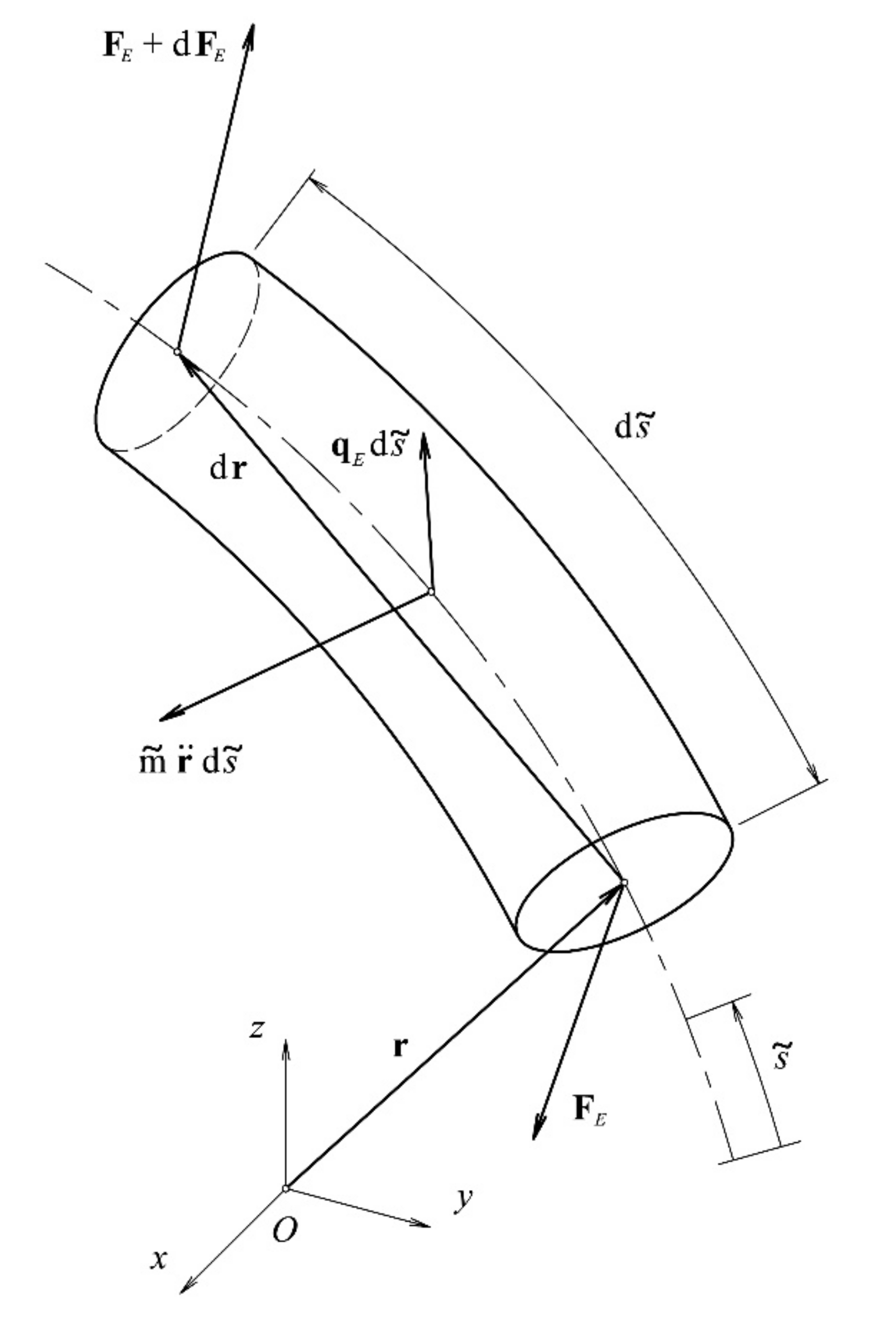
52]. This approach is developed in order to include the influence of the outer hydrostatic pressure due to the seawater on the mooring line. The segment of the mooring line is shown in
Figure 1.
The vector of the effective load
qE contains buoyancy
qB, weight of the mooring line
qW (i.e., dry weight), and hydrodynamic loads
qHThe loads are distributed along the extended length of the segment
. The buoyancy and the weight are defined simply as
where
is the mass per unit length of the segment. Density of the seawater is denoted as
, while
g is the gravity acceleration vector pointing in the opposite direction of the
z-axis of the global coordinate system. Cross-sectional area of the segment is given by
.
The inertial load due to the own mass of the segment is also considered in this model. The vector
denotes the acceleration of the segments (since
represents the second derivative with respect to time), and therefore the term
in
Figure 1 is the inertial load.
The segment of the mooring line is extended to the length
due to the applied loads. The strain
ε, being an axial deformation, is defined as
where
is length of the non-extended segment, i.e., the segment observed in the stress-free configuration of the mooring line. Therefore, the relation between
and
is
Variables
and
in Equations (2) and (3) are related to the extended state of the segment and therefore are dependent on the axial deformation
ε. Poisson’s ratio for synthetic ropes can be assumed as 0.5 [
44]. For this particular value of Poisson’s ratio, the volume of a deformed segment is conserved. Due to this conservation principle, the distributed mass
and the cross-section area
can be defined as
where
A and
m are related to the non-extended state of the segment so that they can be defined as an input.
The hydrodynamic loads
qH from Equation (1) are formulated by the Morison equation:
where ‖ ‖ denotes vector modulus.
CA,
CM, and
CD are the added mass, the inertial coefficient, and drag coefficient, respectively. The cross-section area of the extended segment is denoted by
(as in the expression for the buoyancy). The diameter, which is elongation dependent, is given as
. By the same conservation principle used in Equation (7) for
, the relation for
can be formulated as
The Morison equation given by Equation (8) consists of 3 members. The first member is considered as the inertial force due to the acceleration of the segment through the still seawater. This term is used for the formulation of the added mass. The second member is also a part of the inertial force but is caused by the flow acceleration of the seawater on the fixed segment. The third member is the drag force that is related to the relative velocity of the segment and the seawater flow. The third member is used for the formulation of the damping within the motion equation [
29,
30]. Thus, the drag force is the damping in considerations of the mooring line dynamics.
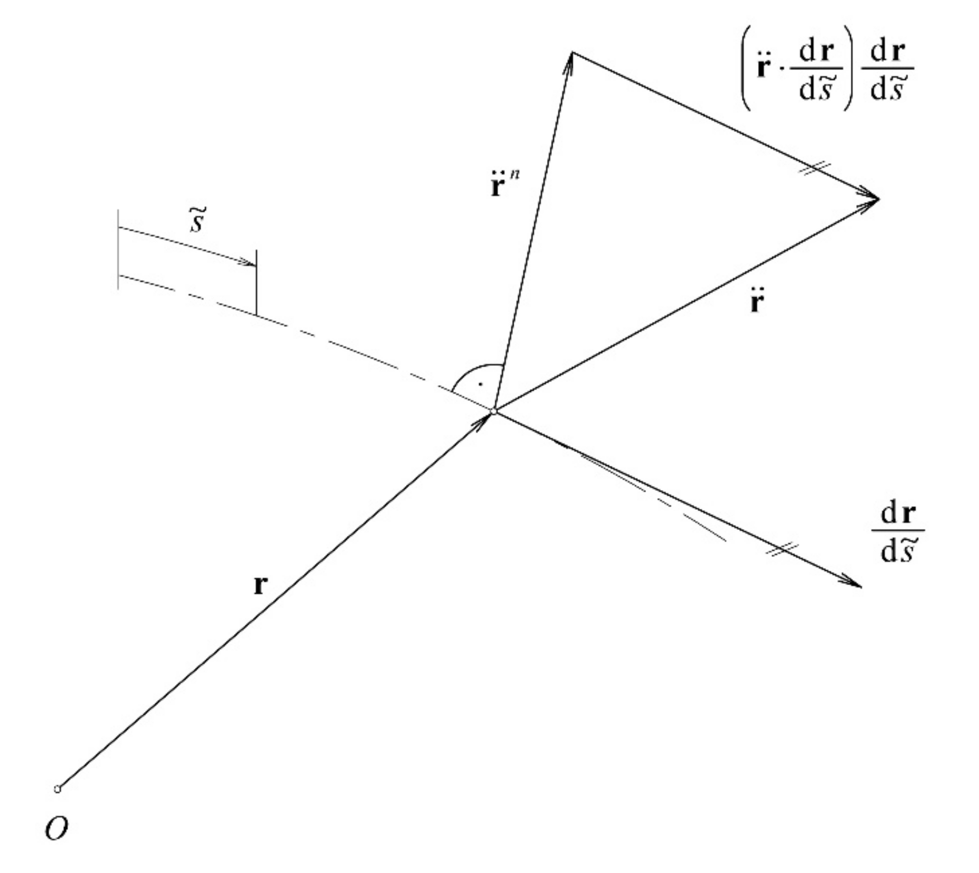
Vector
in Equation (8) is a component of the mooring line acceleration normal to the deformed mooring line
where ∙ denotes a scalar product. The above equation is formulated on the basis of
Figure 2. The second term on the right-hand side is the projection of the total acceleration
to the tangent
of the deformed and extended mooring line. The term
is the unit tangent vector by definition, and thus the second term on the right side is the tangential component of the acceleration. The normal acceleration component can be obtained by subtracting the acceleration tangential component from the total acceleration. In an analogue way,
is defined as the normal component of the mooring line velocity. Furthermore, motion of surrounding seawater is considered through normal components of the water particle acceleration
and velocity
. These vectors are given by
In the present model, the unit tangent vector is obtained by differentiation of the spatial curve r with respect to the extended segment length as . This is in contrast to current practice where the unit tangent is evaluated on the basis of the non-extended segment length in the form , which is a poor approximation for synthetic fibre mooring lines. This is because, as already mentioned, synthetic mooring lines usually undergo a relatively large axial deformation ε and thus great differences in the extended and the non-extended length exist, as given by Equation (5). Therefore, the model developed here has an advantage in calculating hydrodynamic loads since it incorporates a more accurate expression for tangential and normal components of velocities and accelerations.
Normal acceleration given in Equation (10) is now reformulated as
where × denotes a vector product. The new form is obtained by the vector triple product, keeping in mind that
is a unit vector. In the same way, the expressions in Equation (11) can also be reformulated as
as well as a part of the last term in Equation (8)
2.2. Equations of Motion
The force balance on the segment of mooring line leads to
where
FE is the cross-section internal force (see
Figure 1). The balance of moments on the same segment can be expressed as
By inspecting the above equations, one finds that bending and torsional stiffnesses are neglected because only the internal force is considered on the cross-section, i.e., there is no internal cross-sectional moment. Consequently, the rotary inertia terms are not accounted for. Furthermore, the cross-section is assumed to be homogeneous and circular and without shear deformation. Governing equations are treated in the global coordinate system.
Equation (12) contains 2 parallel vectors since the vector product in it equals zero. This fact is used to establish the following relation
where
TE is a scalar value and it represents the effective tension force [
51,
52]. By combining Equations (11) and (13), one obtains the equation of motion of the mooring line:
where the first term on the left-hand side represents the geometric stiffness. Detailed derivations of Equations (13) and (14) can be found in [
48]. The final form of the motion equation is obtained by using Equations (1)–(9) and (12)–(14) as
with
2.3. Discretisation of the Motion Equation
Discretisation of the equation of motion is conducted to define a non-linear finite element for solving the dynamics of the entire mooring line. The axial deformation
ε in Equation (20) is involved in an inconvenient way. A simplification can be obtained by the use of Taylor series expansion
and
Furthermore, the relation between the axial deformation
ε and the effective tension force
TE is given in a simplified manner as
where
AE is the axial stiffness of the synthetic rope, which can be modelled as a non-linear function dependant on the tension. This simplified expression is valid within the assumption that the Poisson’s ratio for synthetic ropes is 0.5 [
44].
By a combination of the above expressions and Equation (20), a form of hydrodynamic loads that is more convenient for discretisation is obtained. It can be written using the index notation as
where prime denotes differentiation with respect to
s and
eijk is the Levi–Civita symbol. All indices used here are in the range from 1 to 3. The unknown variables
TE and
ri are approximated as
with
where
Al and
Pm are shape functions (i.e., polynomials) defined in the interval 0 ≤
s ≤
L, where
L is the length of the finite element (see [
48]). Unknown node displacements
Uil and node effective tensions
λm are expressed as
and
By above equations, the finite element developed here has 3 nodes, 2 end nodes, and 1 mid-node positioned at L/2. Each end node comprises displacements in the sense of 3 translations and 3 rotations in the Cartesian coordinate system and the particular value of the effective tension force as an additional degree of freedom since the tension force is also an unknown value. The mid-node is introduced to give a better approximation of the effective tension over the length of the element so that the mid-node only contains the tension. Overall, the finite element has 15 degrees of freedom, where the only connection nodes are the end nodes, i.e., the mid-node is not a connection node.
The Galerkin method is used for the finite element formulation so that the final form of the discretised motion equation is obtained as
with
and substitutions
where
Qbr and
Wjq are nodal velocities and accelerations of the surrounding seawater, respectively. It should be noted that all integrals in the above set of equations can be evaluated analytically except for the integrals for the drag forces, i.e., the Equations (37)–(39).
In the discretised equation of motion, is the added mass matrix (i.e., tensor) of a mooring line. This added mass is derived from the hydrodynamic loads, i.e., from the first term in Equation (8). It is used for the calculation of inertial forces (due to the motions through seawater) by multiplication with the node accelerations (see Equation (30)). The can be considered as the added mass of a mooring line in the non-extended state when there is no reduction of the mooring line diameter.
has the origin in the same term in Equation (8) and can be loosely referred to as the added mass. This matrix is a direct consequence of the simplification based on the Taylor series expansion where the inconvenient involvement of the axial deformation ε in hydrodynamic loads is resolved (see Equations (21), (23), and (24)). More precisely, it is the second term of the Taylor series from Equation (20), i.e., −2ε, that causes to be populated with non-zero elements. The inertial forces are obtained from this matrix by multiplication with the node effective tension and with (see Equation (30)). In this way, the change of internal forces due to the elongation and the diameter reduction is obtained through the tension . This change is linearly proportional to . Thus, can be comprehended as the linear change coefficients matrix of the added mass.
In an analogous way, is the quadratic change coefficients matrix of the added mass since it originates from the quadratic term 3ε2 of the Taylor series in Equation (20). The quadratic influence on the inertial forces can be noticed in Equation (30) where the term is multiplied by besides multiplication by .
Following a similar pattern, is the node force vector calculated for the non-extended state of the mooring line comprising the drag load part of the hydrodynamic loads, i.e., the second and the third term of Equation (8). and are derived from linear and quadratic terms in the Taylor series (see Equation (22)). Thus, is the linear change and is the quadratic change matrix of the drag load, which are introduced to incorporate diameter changes and the elongation of the mooring line into the hydrodynamic loads. Finally, the analogy stands for the inertial part of the load, i.e., for , , and .
Other matrices and vectors used in the discretised motion equation in Equation (30) are derived and explained in [
48]. In the same paper, an axial elongation condition is presented that is necessary to fully define the mathematical model for solving the mooring line dynamics. In Equation (30), the motion equation is presented with 2 unknowns, the displacements
Uil and the effective tension
λm. Consequently, an additional equation is needed, and it is obtained using the axial elongation condition.
3. Case Studies
Within these case studies, the range of axial deformation from 0.0 to 0.3 was observed, which covers the usual deformations of different types of synthetic ropes in use. These are relatively high values of deformations regarding conventional models used in the current practice. The model proposed here was intentionally developed for such deformations since the diameter reduction and its influence on the hydrodynamic reactions are significant at relatively high axial deformations. Currently, there are no available experimental results or full-scale measurements that are focused on this issue in detail that could be used as a base for validations of the proposed model and comparisons with the current practice. Therefore, an alternative approach based on exact analytical expressions was used. The analytical expressions were derived without any dependency with the proposed model to be used for calculating the inertial and the drag forces. As such, these expressions can be used for independent numerical validations.
To make the derivations of these analytical expressions possible, we considered simple mooring line segments within the case studies, i.e., a straight segment and a curved segment. Both segments had prescribed displacements and were subjected to prescribed fluid velocities and accelerations. Thus, these expressions considered the diameter reduction due to the axial deformation (of observed segments) in the inertial and the drag forces and consequently in the evaluation of the damping and the added mass in an exact analytical way. Finally, these expressions were used to show the achieved improvements of the proposed model over the current practice.
The analytical expressions were not capable of describing the motions of observed segments. As noted, the displacements were prescribed and constant in time. In such circumstances, there is no need for the definition of the boundary conditions. The fluid (i.e., the seawater) velocities and accelerations were also prescribed and constant in time and space. Therefore, the analytical expressions gave the forces for such simplified conditions. For the same simplified conditions, the corresponding forces were calculated with expressions from the proposed model, i.e., from the developed finite element to conduct the numerical validations and to demonstrate archived improvements.
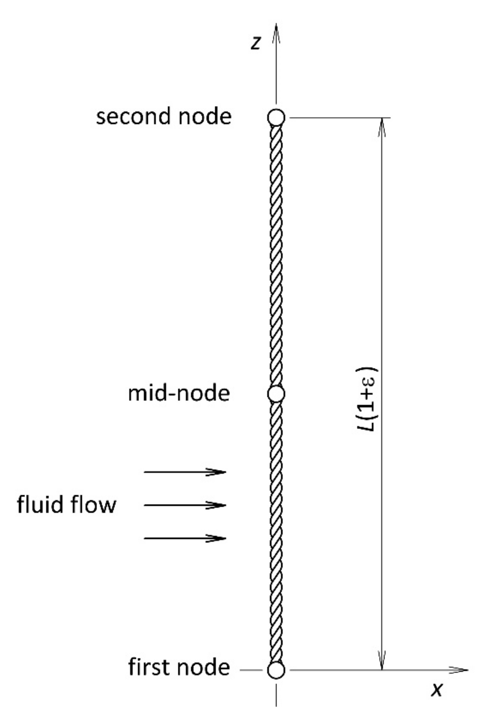
3.1. Straight Segment
To illustrate the effectiveness of the newly developed model, we first observed a straight segment made of synthetic rope. The properties of the rope are listed in
Table 1. The configuration of the segment is shown in
Figure 3. The segment was positioned in the vertical direction. The self-wet weight of the rope was neglected in this case. Only one finite element was used for the segment with an assumption that the value of the axial deformation was constant over the element length. On the basis of the presented assumptions, we formulated the nodal displacements and the nodal tensions as per Equations (28) and (29), respectively:
and
For the evaluation of inertial forces due to the added mass, we assumed a unit lateral acceleration of the segment in the horizontal direction. Similarly, unit velocity of the segment was defined for the calculation of drag forces. In such a simplified case, nodal velocities and accelerations can be expressed as
Here, the two tensors for velocities and accelerations had the same quantities but different measuring units, i.e., for the velocities, m/s was used, and for the accelerations, m/s2.
Similarly, inertial forces are calculated on the basis of unit acceleration (in the horizontal direction) of the surrounding seawater that is constant over the depth. Drag forces are based on unit velocity. Therefore, the nodal values are formulated (keeping in mind the proper measuring units) as
3.1.1. Inertial Forces on the Straight Segment
Calculations of the nodal forces of the observed segment modelled by only one finite element can be conducted by using the already mentioned assumptions and the nodal values defined for the accelerations. Inertial forces due to the added mass, designated as
, are straightforwardly calculated as follows (see Equation (30)):
The expression above takes into account the diameter change and the elongation of the segment through the newly developed terms
and
. Without these terms, the evaluation would be conducted in a manner that is done according to the current practice presented in the literature review as follows:
In order to illustrate the improvement due to the new model, we next present the results of calculations with and without these members.
Since a simple model is considered here, it is possible to analytically determine nodal inertial forces that can be compared with the new model and models from the current practice. In this way, a quality verification of the new model can be obtained. Using the Morison equation and the assumptions of the simple model used here, one can evaluate nodal inertial force as
where
a is the unit horizontal acceleration.
is the extended length of the segment that can be determined as follows (see Equation (5)):
Only half of the extended segment length is included in Equation (49) because a single node receives only half of the total finite element load. The above expression can be simplified using Equation (7) as
Inertial forces due to the acceleration of the surrounding seawater are calculated as follows (see Equation (30)):
where
and
are the additional terms developed in the new model. The current practice models use only the first member
. Analytical approximation of the nodal forces is derived following the same pattern as for Equation (51):
Table 2 presents a comparison between numerical values of the inertial force due to the added mass obtained in different ways. The base for the comparison is the analytically determined force
that can be considered as an exact evaluation of this force (see Equation (51)). The table gives values determined in the usual way, by Equation (48), where the nodal inertial force denoted as
is calculated regardless of the segment elongation and the diameter reduction of the rope. The values obtained by the new model, i.e.,
expressed by Equation (47), take into account the specifics of synthetic ropes regarding their extensibility. The table also gives the percentage of the relative deviation of the numerical models from the analytical solution in order to present the improvement in accuracy of the new model.
Table 3 is formed in an analogous way regarding the inertial force caused by acceleration of the surrounding seawater.
Table 2 and
Table 3 contain the same relative deviations of the numerical models from the exact analytical solutions. The inertial forces are calculated for the simplified straight segment. Such a set-up is the major cause of this. The mathematical models used are very similar in general, but for this simplified set-up are the same. The origins of these models are on the right side of Equation (20) in the first and the second row. The cause can also be found in the definition of the applied accelerations. In
Table 2, where the inertial forces due to the added mass are shown, it is assumed that the segment is in motion with the unit horizontal acceleration immersed in the still seawater.
Table 3, with the inertial forces due to the incoming flow, assumes that the segment is fixed while the incoming flow has the unit horizontal acceleration.
3.1.2. Drag Forces on the Straight Segment
The total drag forces
are also evaluated using Equation (30) as
where
and
are the new terms, whereas
is the term used in the current practice.
For the straight segment, it is possible to formulate analytical expression for the nodal drag forces as
Or by using Equations (9) and (50):
where
v is unit horizontal velocity and | |
denotes the absolute value of a number.
Table 4 and
Table 5 provide comparisons of drag forces as well as their deviation from the analytical values.
Table 4 considers the segment motions, whereas
Table 5 considers the incoming fluid flow. The relative deviations of the numerical models from the exact analytical solutions in
Table 4 and
Table 5 are the same for the same values of the axial deformations. The cause of this is in the simplified set-up used in these case studies. Moreover, the same mathematical model is used for the calculation of the observed drag forces, which has the origin in the last row of the right side of Equation (20). Here, it should be kept in mind that
Table 4 presents the drag forces due to the segment motions with the unit horizontal velocity, while
Table 5 presents the same type of forces but for the fixed segments in the incoming flow with the unit horizontal velocity.
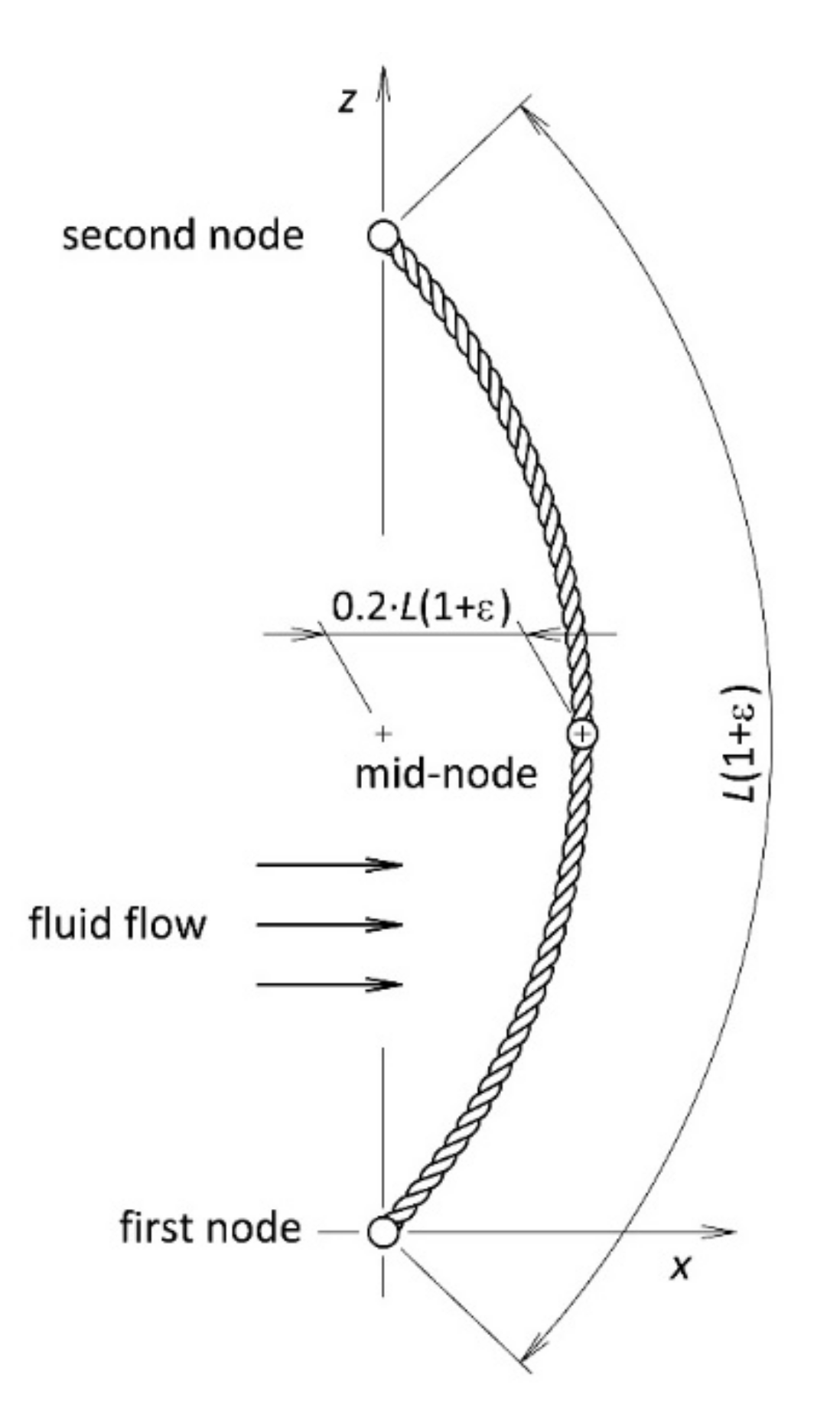
3.2. Curved Segment
To further illustrate the effectiveness of the new model, we next considered a curved mooring line. The same properties of the rope were used as before. Moreover, the same values of horizontal velocity and accelerations were applied. The initial length of the segment was the same as for the straight segment. The configuration of the curved segment is shown in
Figure 4. Again, only one finite element was used with constant values of the axial deformation over the element length. Appropriate nodal displacements needed to be evaluated in the first step, on the basis of the extended length of the segment and a given horizontal deflection. The horizontal deflection was assumed to be 20% of the extended length of the segment given for the mid-node. Calculation of such nodal displacements can only be performed numerically (in this case, using the Newton–Raphson method). Within the method, an effort was made to ensure that the deflection line had as constant a radius of curvature as possible, i.e., the defection line resembled a circular arc.
3.2.1. Inertial Forces on the Curved Segment
Once the nodal displacements of the curved segment were determined, it was possible to calculate the total inertial forces due to the added mass in an analytical way (in the horizontal direction). The Morrison equation was again used to obtain a simple expression
or by using Equations (5) and (7):
In the above expression, the integral can be solved analytically since the
r3 is a third-order polynomial (see Equation (25)). The integration was carried out over the half-length of the segment, since it was assumed again that a single node receives only half of the total finite element load. In an analogue way, inertial forces of the surrounding seawater can be approximated as
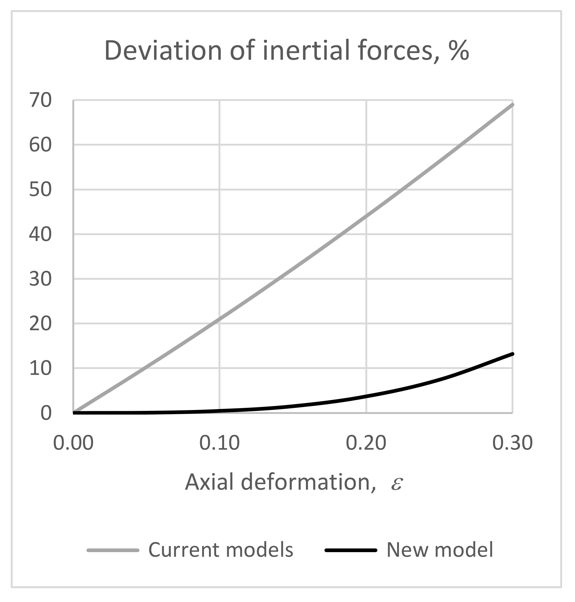
The relative deviation of the inertial forces (for the curved segment) from analytical values is shown in
Figure 5, where current models are compared with the new model.
3.2.2. Drag Forces on the Curved Segment
The expression for the nodal drag forces can be formulated as
and with the use of Equations (5) and (9):
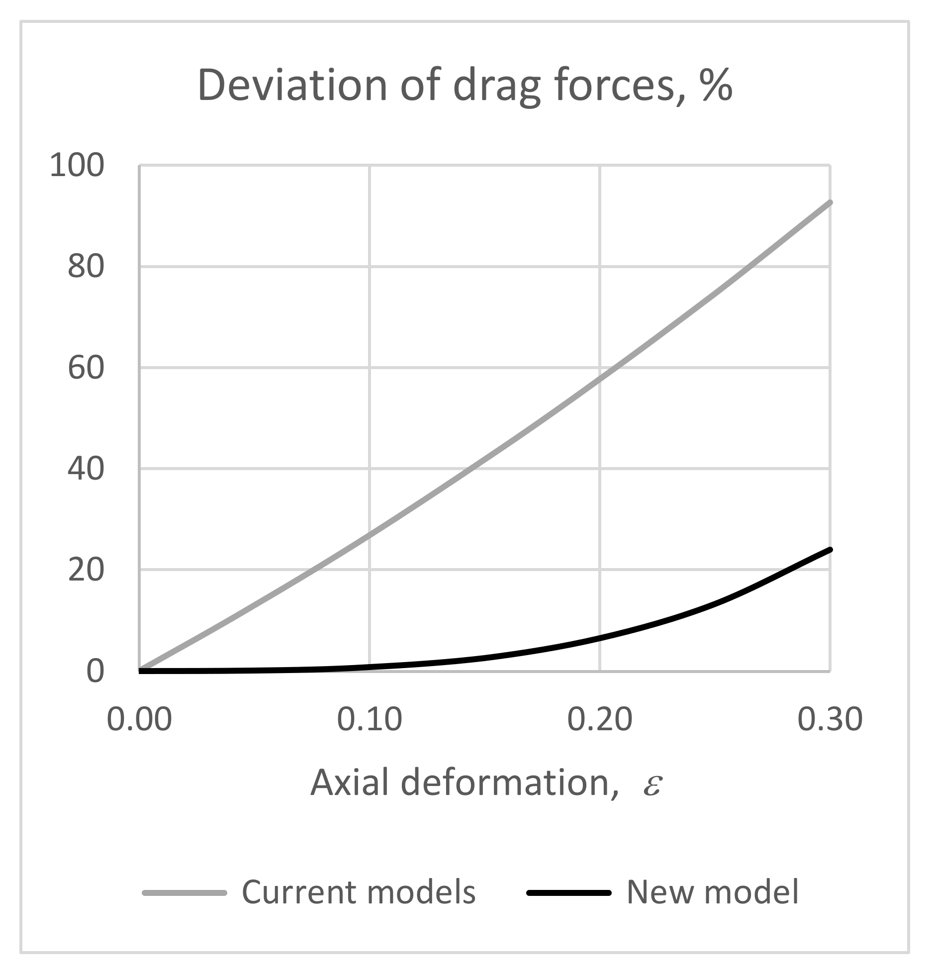
where the integral can be solved analytically. The deviation of drag forces is presented in
Figure 6.
4. Conclusions
This study presents a new finite element intended for modelling of mooring lines made of synthetic fibre ropes. The specifics of the kind of rope was considered in the calculation of damping and added mass. New terms in the finite element formulation were developed and added in order to capture the influence of large values of axial deformation of a mooring line, and consequently the effect of the outer diameter reduction in calculation of hydrodynamic reactions. The new terms in the formulation can be comprehended as a linear and a quadratic change of hydrodynamic reactions due to the deformations of synthetic ropes. The current practice does not consider these deformations and therefore overestimates forces due to damping and the added mass.
In order to present the effectiveness of the new model, we studied a set of simple mooring lines, i.e., mooring line segments, namely, a straight and a curved segment with predefined deflections. For these simple segments, analytical formulas were derived that were exact expressions for the hydrodynamic reactions. These analytical expressions were used as a base for comparison of the current practice model and the new model.
Damping forces due to a prescribed motion of a segment and due to an incoming flow were evaluated. The range of the axial deformation from 0 to 0.3 was considered. Comparisons revealed that the current practice significantly overestimated damping forces. For the axial deformation of 0.2, this overestimation was approximately 58% in comparison to the analytical results. The new model had a much better correlation with the analytical calculations, and the overestimation was only 6.5%.
Inertial forces caused by prescribed accelerations were also calculated. The same range of axial deformations 0 to 0.3 was considered. The current practice models overestimated these forces by approximately 44% for both segments. The new model once again achieved significantly better correlation with the analytical calculations. The overestimation in this case was 3.7%, which clearly demonstrated the effectives of the new model.
In general, the new model reduced the overestimation of the hydrodynamic reactions by one order of magnitude for the set of a simple case studies considered. Nevertheless, there was room for improvement. This was because with axial deformations approximately above 0.17, the overestimates of the new model were above the usual engineering acceptable error of to 2%. Moreover, the new model is numerically more demanding and should be tested within a coupled dynamic analysis of a mooring system and a moored vessel since the new members in the finite element formulation are the tensors up to the sixth order. This can be a direction for future investigations.


