Abstract
Mean wave period (MWP) is one of the key parameters affecting the design of marine facilities. Currently, there are two main methods, numerical and data-driven methods, for forecasting wave parameters, of which the latter are widely used. However, few studies have focused on MWP forecasting, and even fewer have investigated it with spatial and temporal information. In this study, correlations between ocean dynamic parameters are explored to obtain appropriate input features, significant wave height (SWH) and MWP. Subsequently, a data-driven approach, the convolution gated recurrent unit (Conv-GRU) model with spatiotemporal characteristics, is utilized to field forecast MWP with 1, 3, 6, 12, and 24-h lead times in the South China Sea. Six points at different locations and six consecutive moments at every 12-h intervals are selected to study the forecasting ability of the proposed model. The Conv-GRU model has a better performance than the single gated recurrent unit (GRU) model in terms of root mean square error (RMSE), the scattering index (SI), Bias, and the Pearson’s correlation coefficient (R). With the lead time increasing, the forecast effect shows a decreasing trend, specifically, the experiment displays a relatively smooth forecast curve and presents a great advantage in the short-term forecast of the MWP field in the Conv-GRU model, where the RMSE is 0.121 m for 1-h lead time.
1. Introduction
Wave parameters, especially significant wave height (SWH) and mean wave period (MWP), affect designing marine facilities, such as floating key equipment operations and ship-mooring installation, as well as important environmental factors in marine engineering design. In addition, SWH and MWP are not only an indispensable part of wave energy studies, but also their functional form can constitute pressure, velocity, and acceleration caused by wave-induced force [1].
Commonly, wave forecasting methods are organized into two main categories: numerical methods and data-driven methods. Numerical models based on energy balance, such as wave action model (WAM [2]), simulating waves nearshore modeling (SWAN [3]), and WAVEWATCH III [4], are widely applied to simulate wave conditions. When they forecast the MWP, the wave spectrum is generally utilized. Rogers et al. [5] proposed an adjustment of the parameter weights in the whitecapping formulation to improve the forecasting of low-frequency (0.05–0.19 Hz) energy in response to the problem of SWAN underestimation of the wave period. Amrutha et al. [6] used the WAVEWATCH III model to evaluate deepwater buoy data measured at 15.0000 N, 69.0000 E and demonstrated that the MWP was overestimated and underestimated at high (SWH > 2 m) and low (SWH < 1 m) sea state conditions in the nearshore, respectively. Additionally, the SWAN model has been successfully employed in the evolution of wind waves in coastal areas, lakes, and estuaries, but the simulated wave periods are generally less accurate than the predicted wave height [7]. Moreover, numerical methods require a lot of computational work and effort as well as relevant professional knowledge.
Data-driven methods, such as statistical and machine learning methods, have focused more on SWH and less attention on MWP. They typically apply correlations in the time series to make forecasts without numerical solutions. The statistical method compiles and analyzes time series to further forecast future trends by analogy or extension based on the development process, direction, and trend reflected by historical data. The main methods commonly used are the autoregressive (AR), the autoregressive moving average (ARMA), and the autoregressive integrated moving average (ARIMA) models. Guedes Soares and Ferreira [8] focused on simulating a time series of SWH measured on the Frigg platform in the North Sea using the Box–Jenkins AR models. They [9] simulated a binary series of SWH and MWP in 2000 and proved that the simulations exhibited a correlation between the two parameters, which is a feature that cannot be reproduced by univariate sequence. The simulations of both models can be generalized and applied to other types of relevant data sets. Reikard [10] proposed the time-varying regressions to forecast the wave height and periods separately, and combined the forecasts to predict the flux, which have fairly high forecasting errors compared to other forms of alternative energy sources due to the inherent variability of the data. Additionally, AR-based on linear and stationary theories have limitations in forecasting nonlinear and non-stationary wave parameters. Duan et al. [11] described a hybrid empirical model decomposition-AR model for nonlinear and non-stationary wave forecasting, which outperforms the AR model.
On the other hand, machine learning methods seem to be a good modeling tool for stochastic processes, and they are widely applied to the forecasting of non-stationary and nonlinear time series. Especially, if they are combined with statistical techniques, they can be faster and, in some cases, more accurate methods. See, e.g., Stefanakos [12], where nonstationary stochastic modeling has been combined with FIS/ANFIS in the prediction of SWH, wind speed (WS) and peak period. Kalra et al. [13] proposed a technique based on the radial basis function (RBF) type of the artificial neural network to estimate the daily SWH at a coastal location based on the wave height sensed by a satellite along its tracks. Prahlada and Deka [14] developed a wavelet decomposed neural network model in order to make predictions of time series. Berbić et al. [15] used artificial neural network and support vector regressive (SVR) to provide the possibility of real-term SWH. Yang et al. [16] presented an optimal hybrid forecasting method based on back propagation neural network and cuckoo search algorithm, and proved that the proposed hybrid model performs effectively and steadily. Fan et al. [17] employed a long short-term memory (LSTM) network for the quick prediction of SWH with higher accuracy than a conventional neural network. Kaloop et al. [18] integrated wavelet, particle swarm optimization, and extreme learning machine methods for estimating the wave height and found better performance in model results for coastal and deep-sea areas regions up to 36-h lead times. The bulk of the studies on ocean wave parameters in data-driven are related to SWH and the studies related to MWP are limited. Özger [19] combined wavelet and fuzzy logic methods for the forecasting of both variables. Wu et al. [20] proposed and developed a physics-based machine learning model in detail to do multi-step-ahead forecasting of wave conditions for marine operations.
LSTM is widely considered for the problem of forecasting time series data, while gated recurrent unit (GRU), as a variant of LSTM, has a more concise structure, faster training speed, and maintains the properties of LSTM that can prevent gradient explosion, gradient disappearance, and local extrema. Rui et al. [21] applied the LSTM and GRU models to forecast short-term traffic flow, and the experimental results showed that GRU has better performance than LSTM on 84% of the total time series. Song et al. [22] proposed a dual path GRU network for sea surface salinity prediction from the Reanalysis Dataset of the South China Sea, and demonstrated the feasibility and validity of the model.
As mentioned above, for wave conditions, studies mainly lie in the forecasting of SWH, with little focus on MWP and even less attention to temporal and spatial characteristics. In this paper, the idea of convolution is incorporated into the gated recurrent unit (GRU) model to form a convolutional gated recurrent unit (Conv-GRU) model with spatiotemporal characteristics, thus providing the possibility to the MWP field in the South China Sea. The correlations among the variables SWH, MWP, WS, mean wind direction (MWD), and sea surface temperature (SST) are investigated to obtain highly correlated field forecasting input characteristics with MWP. Subsequently, six points that can roughly represent the characteristics of the study area are selected to further analyze the forecasting capability for different location features, and experiments with 1, 3, 6, 12, and 24-h lead times are conducted to observe the performance of the model. Finally, six consecutive moments at 12-hour intervals are chosen for drawing, so as to more vividly express the forecasting results of the field data in space as well as the variation in time.
In Section 2, the experimental data and details of six points at the study area are depicted, and the GRU and Conv-GRU forecasting models are described. In Section 3, correlation analysis between input variables, results of six-point time series, and field data experiments are introduced. Conclusions are summarized in Section 4.
2. Data and Methods
Ocean dynamic parameters, SWH, MWP, WS, MWD, as well as SST, are obtained for every 1-h interval in the South China Sea from the ERA5 global atmospheric reanalysis produced by European Centre for Medium-Range Weather Forecasts (ECMWF). The ERA5 is based on the more robust Huber norm, providing background error estimates for deterministic HRES DA systems with the hourly high-resolution output throughout, 3-hourly uncertainty information, and timely and preliminary within 5 days real-time available product characteristics [23]. The time span of the data utilized in the paper is 1600UPC on 11 February to 0700UPC on 30 November 2018, with a data volume of 7000. All data are independently partitioned into a training set (first 6000) and a test set (subsequent 1000) to avoid peeking too much about the sample characteristics in the test set and subsequently bringing in bias in the predictions. The red box represents that, in the South China Sea, the study area is selected from 109–120 E and 10–21 N, as shown in Figure 1, where the spatial resolution is 1 longitude × 1 latitude grid data.
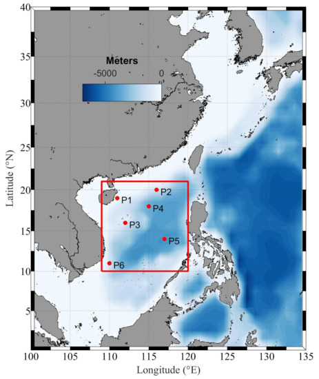
Figure 1.
The geographic of the study area and six points as well as bathymetry, where the red square represents the study area and the six red dots indicate representative locations.
The South China Sea has complex geographical characteristics, such as varying degrees of bathymetry, wide sea areas, alternating monsoons, and so on. Six points were selected to ensure that a wide range of geographical locations and different geographical features could be covered, including P1 with shallow water around Hainan Island, P2 in the northeast of the Dongsha Islands with rich oil resources, P3 in the Paracel Islands, P4 and P5 in the northwest and southeast of Zhongsha Islands, and the latter is placed in deep water and P6 with many islands in the Spratly Islands, as shown by the six red points in Figure 1. The Spratly Islands have the widest range and belong to the equatorial monsoon climate zone. In contrast, the Zhongsha Islands are second only to it and they are located in the central waters of the South China Sea and have tropical monsoon and equatorial climates, which makes the situation more complicated and has a certain seasonality. Therefore, two points (P4 and P5) are chosen as features in the Spratly Islands. Table 1 lists the detailed locations and related information of six points.

Table 1.
The latitude, longitude, water depth, and the maximum and minimum Mean wave period (MWP) at six points.
2.1. Gated Recurrent Unit Networks (GRU)
A recurrent neural network (RNN) is a superset of feed-forward neural networks, augmented with the ability to transmit information across time steps. They are a rich family of models with the ability to represent complex nonlinear relationships between inputs and outputs, capable of almost arbitrary computations [24]. However, RNN suffers from the problems of gradient explosion and disappearance. In the past few years, the long short-term memory (LSTM) networks with obvious advantages have shown record performance on various tasks, such as image processing [25], language translation [26,27], and handwriting recognition [28,29].
Compared with LSTM, GRU, was presented by [30], not only has a more concise structure, better effect, and saves more running time and computing power, but also retains the original advantages of the LSTM model. It solves the problems faced by traditional RNN, and generates long-term continuous cell units by self-circulation through the feedback method to learn faster. The GRU model is similar to the general form of a neural network, input layer, hidden layer, and output layer. The hidden layers are GRU units, which are connected end to end, and the input from layer to layer is the output of the previous layer, resulting in the output of the model.
The GRU model contains two gates, the update gate and the reset gate , to control the input , memory unit , and output . The memory unit can simultaneously control long-term information and local information. The reset gate is used to control how much past information is forgotten, i.e., the extent to which the hidden layer state at the previous moment is added to the current candidate hidden layer state . The update gate determines how much past information is passed to the future, i.e., how much the hidden layer state at the previous moment is updated to the current hidden layer state . The larger the update gate, the more the state information at the previous time step is remembered. The smaller the reset gate, the more information in the previous state is forgotten [31].
where · is matrix multiplication, U and W with different subscripts represent the weight between corresponding layer structures respectively, b indicates the bias, is the sigmoid function, denotes the internal candidate state, and are the output of the hidden layer at the time t and .
The calculation of the local information available at the current time t is directly extracted from the long-term information through the reset gate , that is, the product of the reset gate and the hidden layer output at the previous moment . Subsequently, the local information is spliced with the external input , and then the weight is multiplied by to form the current candidate hidden layer state.
where ⊙ represents the product of matrix elements, denotes the hyperbolic tangent function, indicates the internal candidate state.
The calculation of the new long-term information combines the long-term information of the previous step with a part of the current information of this step through the weight.
Finally, linear connection is employed to process the hidden layer output to get the output of the model.
where is the output of this layer at time t.
2.2. Convolutional Gated Recurrent Unit Networks (Conv-GRU)
The starting point of convolutional neural network (CNN) is the neurocognitive machine model. The classic LeNet was developed by [32], when the convolutional structure has already appeared. CNN is a feed-forward neural network consisting of one or more convolutional layers and a fully-connected layer at the top, and also includes associative weights and pooling layers. Its artificial neurons can respond to surrounding units in a part of the coverage area and have excellent performance in image and speech recognition. By training end-to-end networks with paired inputs and desired output instances, problems that require complex pipelines of highly tuned algorithmic building blocks become solvable at unprecedented levels of performance because of the rapid development of CNNs [33].
Convolution is the sum of two variables after being multiplied within a certain range. In the continuous case, it refers to the integral of the product between variables, in the discrete case, it is the weighted sum of the scalar set arranged in a regular grid. Its purpose is to find the output signal of a certain input signal after the action of linear time-invariant systems. Linearity means that any input signal can be superimposed, i.e., it can be decomposed into multiple impulse signals, while time-invariant is essentially the invariance of time translation, which indicates the conservation of energy. By replacing the convolution operation with the connection operation between the units, it can be inferred that the formula of the Conv-GRU model in which the concept of convolution in CNN is considered in the GRU model is represented by Equation (5).
where ∗ represents convolutional multiplication.
The main frameworks of the GRU and Conv-GRU models are input layer, hidden layer, and output layer. The former predicts single point time series while the latter forecasts field data, so they have different types of outputs. A particularly obvious difference between them is the computation of the hidden layer, which operates on the input signal through different connections for the ultimate purpose of forecasting time series or field data, as shown in Figure 2.
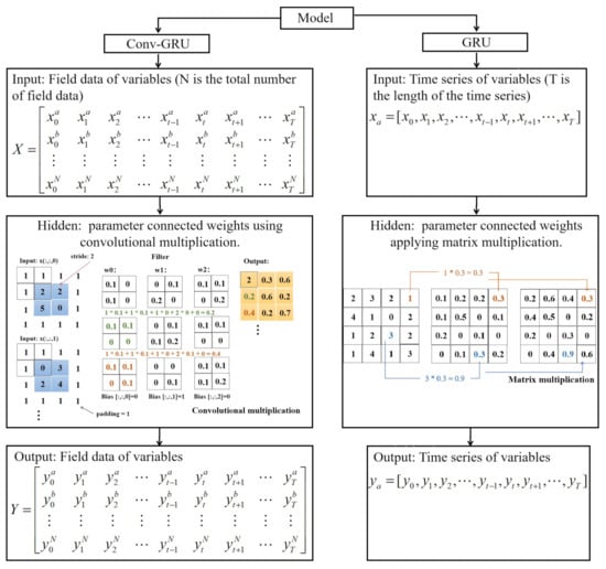
Figure 2.
A simple flow and typical difference between gated recurrent unit (GRU) and Conv-GRU.
Subsequently, we will explore the model performance with time series and field data as the entry point.
3. Results
3.1. Experimental Preparation
In the Conv-GRU model, the input data are the form of matrix, while the extracted data exist in terrestrial points, i.e., NANs, which are replaced by 0 considering the physical knowledge and experimental needs. Moreover, the input variables under different dimensions are normalized to reach the same order of magnitude, subsequently, the output contents are denormalized to return to the previous order of magnitude, where the formulas are shown as Equations (6) and (7), respectively. These operations can ensure the integrity of the data, accelerate the convergence speed and improve the learning efficiency of the model.
where and are before and after normalized data, and represent the mean and variance of , respectively.
Similar to Equation (6), denotes the final output, represents the model output, and are the mean and variance of .
Several statistical parameters such as Bias, root mean square error (RMSE), the scatter index (SI), and the Pearson’s correlation coefficient (R) are introduced to evaluate the effectiveness and accuracy of all models. Within the statistical quantities, the specification of Bias, RMSE, SI, and R are given in [34]. Here the bias is calculated by subtracting forecasting from observation to measure the accuracy of the model. Therefore, the minus sign in the bias indicates an overestimation of the model. RMSE describes the average deviation between forecasting and observation. SI is the quotient between the RMSE and the mean of forecasting, which represents the overall accuracy. R can measure the linear relationship between two data. It is more sensitive to outliers than those the mean [35]. The formulas are shown in Equation (8).
where and represent observation and forecasting at time t, and denote the mean of and respectively, and n is the total number of test samples.
The training phase is a process of learning the required weights for each local mapping and function fit. In the feedback process of the models, the mean-square error (MSE) is chosen as the loss function. The adaptive moment estimation (Adam), which can replace the traditional stochastic gradient descent algorithm, is selected as the optimization method with a learning rate of 0.0006. The main parameters of the models, the iterative time, the batch size, the number of hidden layers, the number of nodes in the hidden layer, the activation function, and the convolution kernel size, were adjusted during the experiment. The final experimental parameters results are shown in Table 2.
Table 2.
Parameters of the Conv-GRU and GRU models.
3.2. Correlation of Input Variables
To avoid the inclusion of redundant information and the omission of important information, the correlations between the input variables MWP, SWH, WS, MWD, and SST need to be further explored. Figure 3 shows the correlation matrix between the input variables at each point from P1 to P6, thus enabling a quantitative understanding of them. Furthermore, the correlation of the input parameters to MWP would like to be expressed qualitatively and graphically.
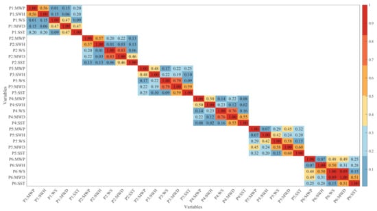
Figure 3.
Correlation matrix of input variables MWP, significant wave height (SWH), wind speed (WS), mean wind direction (MWD), and sea surface temperature (SST) from P1 to P6.
Table 3 lists nine experiments for different input variables predicting the output variable MWP using the Conv-GRU model with a 6-h lead time so as to select the wave characteristics highly correlated with the MWP for subsequent experiments. Of these, experiments from 1 to 5 represent univariate inputs, experiments from 6 to 8 are bivariate inputs, and experiment 9 denotes a multivariate input.
Table 3.
Details of the input variables for experiments 1 to 9.
The experimental results are presented in Figure 4 and Figure 5, respectively, according to the number of input variables. The former shows scatterplots of observation and forecasting obtained after the univariate experiments, while the latter depicts the results of multivariate experiments.
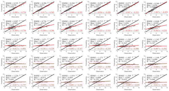
Figure 4.
Scatterplots of observation and forecasting obtained in different experiments using the Conv-GRU model with a 6-h lead time. The subplots from top to bottom represent the first five experiments in Table 3, respectively. The subplots from left to right correspond to P1 to P6. The red line indicates a linear fit and the black line means a full correlation.
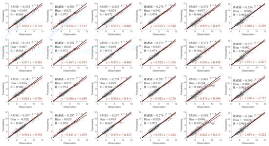
SWH has a high correlation with MWP, SST has a small effect on MWP, while MWD and WS have a similar result to MWP in Figure 3. This conclusion can be verified from Figure 4. From top to bottom, input variables MWP, SWH, WS, MWD, and SST forecast MWP in the Conv-GRU model with a 6-h lead time experiments demonstrate a drop result. The six points from left to right show different effects, which will be analyzed in detail in Section 3.3 in terms of numerical and physical phenomena.
The Conv-GRU experiment of multivariate MWP and SWH, MWP and WS, MWP and MWD, and MWP, SWH, WS, and MWD forecasting univariate MWP are given from top to bottom in Figure 5. A comparison with the top image in Figure 4 shows that the experimental effect of adding SWH to the input feature is better than that of a single MWP, and the addition of MWD and WS makes the experimental result a little worse, except for P2, the reason for this phenomenon will be explained in Section 3.3, while the experimental results of four input parameters also show a slightly worse result. It indicates that considering adding highly-correlated variables to the input features will enhance the forecasting effect, while the addition of weakly correlated variables is equivalent to a kind of redundant information, which will slightly reduce the forecasting ability. Additionally, when it is necessary to simulate the MWP of the ocean state simultaneously, the conclusion that the univariate autoregressive model of SWH needs to be generalized to the bivariate model is obtained by [9]. In Figure 6, the running time increases approximately exponentially as the input characteristics increase. Based on the dual considerations of efficiency and effectiveness, the bivariate SWH and MWP are selected as the input features of the experiment.
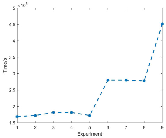
Figure 6.
The running time variation plots of experiments 1 to 9 in Table 3.
3.3. Explore the Time Series at Six Points
According to the conclusions obtained in the previous section, the GRU and Conv-GRU models were performed for six points of input features SWH and MWP with 1, 3, 6, 12, and 24-h lead times to explore the forecasting ability of the model. The input features are composed of the time series SWH and MWP. The target series and output features express the observed and forecast results of the time series MWP with an L-h lead time, respectively. For simplicity, the input features are noted as , the target series is marked as , and the output feature is written as , where represents the number of spatial points, and denotes the length of the time series. Moreover, a random column is chosen as an example to fully characterize the model meaning as shown in Equations (9)–(11).
To characterize the forecasting power of the model, we compare it with the other methods mentioned in the introduction and GRU. All three methods have bivariate inputs SWH and MWP. Figure 7 exhibits the performance of these methods with a 6-h lead time and demonstrates that the Conv-GRU model has the best forecasting performance.
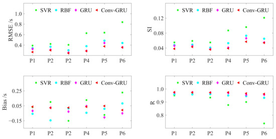
Figure 7.
Performance of the SVR, RBF, GRU, and Conv-GRU models.
Table 4 lists the statistical properties of the GRU and Conv-GRU models. The numerical results show that the models have different perturbation and forecasting ability for the six points, and the performance of GRU is inferior to Conv-GRU.
Table 4.
Six points of performance at different lead times in the Conv-GRU (GRU) model.
It is noteworthy that, when plotting the observation and forecasting effects, we plot the observation last to highlight their overlap and goodness-of-fit with the forecast curves, as shown in Figure 8. Observing the sub-graph, the GRU model can forecast MWP, but the fluctuate greatly for high and low peaks, which is a little meaningful for MWP. Convolution is taken into account in the original model to obtain an improved forecasting model with spatiotemporal characteristics. Below we will analyze the six-point one by one to explore the forecasting strength of the models at different locations.
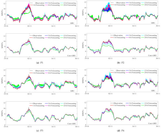
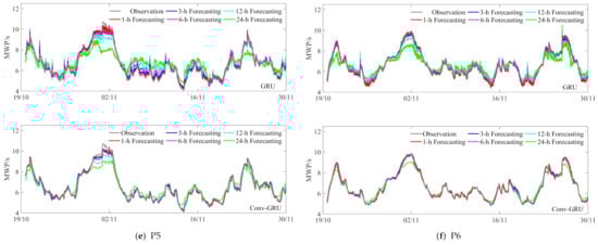
Figure 8.
Time series plots of the GRU and Conv-GRU models at six locations, where (a–f) represent P1-P6. Each subplot is split into two plots, the upper one showing the experimental results obtained from the GRU model, on the contrary, the lower one reflecting the content obtained by the Conv-GRU model. The gray and red (blue, magenta, cyan, green) curves depict the observation and 1-h (3, 6, 12, and 24-h) forecasting under the different models, respectively. The X-axis is the time series corresponding to the test set in 2018.
Compared with the other five points, P1 is far from the sea center, almost inland, and belongs to the shallow sea area, which is affected by many factors and will produce refraction, diffraction, and reflection. In addition, in the test set, the MWP is larger than 8 s except for the time near 2nd November, and the rest of the time is smaller than 8 s, which is a good situation compared with the more fluctuating curve, so the forecasting result of P1 is slightly better than P4.
It can be observed from Figure 5 that the forecasting effect of P2 is slightly worse when SWH is added to the input feature, while the forecasting effect of P2 is improved when the WS is considered in the input feature. This phenomenon indicates that the wind has a greater impact on MWP than SWH at P2. After reviewing the data, it was found that P2 encountered super typhoon TUYU at 2100UPC on 31 October 2018 in Figure 9, which brought stronger and more sustained winds [36]. This implies that when the wind is severe, it has a greater impact on MWP, while SWH is also affected by the wind and has a slightly less impact on MWP. When the wind is calm, its impact on MWP is much smaller, SWH plays a major role and has a greater impact on MWP. Thus P2 has a bit of worse effect.
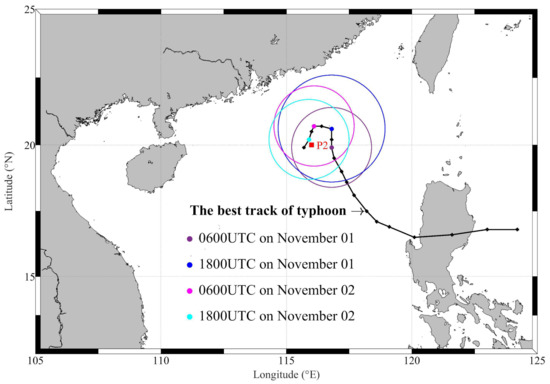
Figure 9.
Track of typhoon YUTU from 1200UPC on 29 October to 2400UPC on 2nd November 2018. The green (blue, magenta, cyan) circle represents the radius of major storm axis, which is 45 (35, 35, 35) nm.
P3 is situated at the center of Paracel Islands, where the wind blows all year round. Compared with other locations, it has sharper wave peaks, shorter periods, shorter wavelengths, and shorter peak lines, and is subject to winds significantly smaller than the strong winds generated by typhoons, so that SWH dominates and the forecasting are closer to the observation, so the result of the bivariate SWH and MWP improves and dominates the performance.
P4 and P5 are placed in the Zhongsha Islands, but P5 is located in deep water, and the wave conditions between them depend on changes in the wind field. In winter, it is the northeast monsoon period, and the sea area produces larger waves mainly in the northeast direction under the action of the strong northeast monsoon. The MWP is 5.4 to 11.5 s, of which 6 to 8 s account for about 57%, and more than 8 s accounts for about 33%. Summer is the southwest monsoon period, and its wave type is mainly mixed waves with similar frequency of wind waves and swell waves. The size of the waves is lower than in winter, with an MWP of 4.5 to 14 s, of which about 53% are 6 to 8 s and about 27% are more than 8 s. It can be seen from Figure 8 that both points produce more high and low peaks at the time series. P5, although it has a smaller peak, has more high and low peaks than P4. In contrast, P4 has a larger peak and fewer high and low peaks. This makes the errors generated by the high and low peaks accumulate, resulting in different and slightly worse forecasting results.
Located in the Spratly Islands, P6 belongs to the equatorial monsoon climate zone. Under the influence of the northeast monsoon, southwest monsoon, subtropical high pressure, tropical convergence zone, and tropical cyclone, it has formed year-round high temperature and high humidity, heavy wind and small fog, and obvious dry and wet seasons. The MWP at P6 has periodic and monsoon influences and its wave peaks are relatively rounded and larger than 8 s, which further lead to relatively poor forecasting results.
Comparing the upper and lower subplots at each point, we can see that the forecast curves of the Conv-GRU model are smoother and more stable, and the high and low peaks do not produce sharp forecasts. The red and blue curves almost overlap with the observation except for a slightly worse fit at larger values, and the pink curve appears slightly overestimated at the location of minimum. Overall, with the lead time increases, the forecast curves gradually approach the central position, which are particularly obvious for 12 and 24-h lead times. The results illustrate that considering convolution not only improves the forecast deficiencies of the GRU model, but can also demonstrates that the Conv-GRU model can extract spatial information from the MWP field data and retains the ability of GRU to make long-term series forecasts. Subsequently, it should be pointed out that different lead-time forecast curves have regular forecast lags. The longer the lead time, the more obvious the lag of the forecast curve. In addition, all RMSE and SI gradually increase, while R gradually decreases.
3.4. Analysis of MWP Field
The comparison between the numerical results of the Conv-GRU model in Table 5 shows that RMSE, SI, and Bias increase with the increase of lead time, while R decreases and shows a positive correlation between the forecasting and observation. When the lead time is less than 12 h, RMSE, SI, and Bias are less than 0.335 m, 0.051, and 0.035 m while R is more than 0.973. When the lead time is more than or equal to 12 h, RMSE, SI, and Bias are more than 0.515 m, 0.078, and 0.038 m while R is less than 0.934. It can be explained that the model shows a feasible and effective numerical result, and performs well in short-term MWP forecasting.
Table 5.
Statistical indicators in the Conv-GRU model at different lead times.
In order to show the field forecasting effect of the Conv-GRU model more clearly and intuitively, starting from the moment when P2 encounters the typhoon from 2100UPC on 31 October 2018, the experimental results of 1, 3, 6, 12, and 24-h lead times every 12-h are drawn. Figure 10 presents the results of the field forecasts and the temporal variations. In time, P2 as an example, the MWP starts to increase in the short term until 10.300 s, then decreases and finally stays around 8 s. Spatially, the larger MWPs are mostly distributed in the Zhongsha and Spratly Islands. Finally, it can be pointed out that there is a high degree of similarity between observation and forecasting, and as the lead time increases, the forecasting results become worse, which is consistent with the obtained numerical results. The above results show that the Conv-GRU model presents better performance and higher accuracy for short-term forecasting of MWP field data.
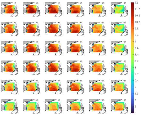
Figure 10.
Comparison the forecasting and observation with the MWP field data, in which the results from top to bottom correspond to the observation and the forecasting with 1, 3, 6, 12, and 24-h lead times, and from left to right are the moments every 12-h from 2100UPC on 31 October 2018. The X-axis and Y-axis respectively represent the latitude and longitude of the study area.
4. Conclusions
The planning and designing of coastal structures are closely related to MWP. The Conv-GRU model, as a data-driven method, is a novel algorithm of field forecasting with spatiotemporal characteristics by combining convolution and the GRU model, which not only retains the long-term time series forecasting characteristics of the GRU model, but also utilizes convolution to extract local spatial information. In this paper, the SVR, RBF, and GRU models are employed for comparison to explore the forecasting capability and accuracy of the Conv-GRU model. Secondly, the correlations between wave dynamics parameters MWP, SWH, MWD, WS, and SST are investigated to select highly correlated variables. The bivariate MWP and SWH were chosen as input features for MWP forecasting experiments with the lead times of 1, 3, 6, 12, and 24-h for the single-point time series (P1-P6) and six consecutive moments at every 12-h intervals. Additionally, RMSE, SI, Bias, and R are applied as the evaluation criteria for the overall forecast error.
The experiments show that the Conv-GRU model can effectively extract the spatial correlation of field data and time information of single-point time series, which proves the feasibility and effectiveness of the model in forecasting MWP field data. With the lead time increasing, as a whole, the forecast error of the Conv-GRU model increases from 0.136 to 0.774 m for RMSE, from 0.020 to 0.117 for SI, from 0.031 to 0.046 m for Bias, decreases from 0.996 to 0.843 for R, and the forecast curves gradually approach the center. Unexpectedly, it is found that WS is only second to SWH in terms of correlation for MWP, but its effect on MWP is greater than that of SWH when the wind is severe, on the contrary, it is slightly less when the WS is calm and SWH plays a major role. In addition, in the Conv-GRU model, the forecasting results obtained by the model are smoother, which makes up for the sharp effect of the GRU model at the peak. Overall, the Conv-GRU model has spatiotemporal characteristics and performs well in short-term MWP field forecasts. Furthermore, for long-term forecasts, the model performance results will be slightly worse, and further work can be focused on long-term MWP field forecasts. Moreover, other spatiotemporal models, such as PredRNN++ [37], can be added and applied to the forecasting of wave conditions to verify the effectiveness and superiority of the Conv-GRU model.
Author Contributions
Conceptualization, J.W.; methodology, J.W.; investigation, J.W.; resources, J.W.; data curation, J.W.; supervision, J.W.; project administration, J.W.; funding acquisition, J.W.; software, T.Y.; formal analysis, T.Y.; writing—original draft preparation, T.Y.; visualization, T.Y.; writing—review and editing, T.Y. Both authors have read and agreed to the published version of the manuscript.
Funding
This work was supported by the National Key Research and Development Project of China [grant number 2016YFC1401800]; the Shandong Provincial Natural Science Foundation [grant number ZR2020MD060]; the Fundamental Research Funds for the Central Universities [grant number 19CX05003A-5].
Institutional Review Board Statement
Not applicable.
Informed Consent Statement
Not applicable.
Data Availability Statement
Data used can be accesses via ERA5 website.
Conflicts of Interest
The authors declare no conflict of interest.
References
- Jesbin, G.; Sanil, K.V. Climatology of wave period in the Arabian Sea and its variability during the recent 40 years. Ocean Eng. 2020, 216, 108014. [Google Scholar]
- The Wamdi Group. The WAM model—A third generation ocean wave prediction model. J. Phys. Oceanogr. 1988, 18, 1775–1810. [Google Scholar] [CrossRef]
- Booij, N.; Ris, R.C.; Holthuijsen, L.H. A third-generation wave model for coastal regions: 1. Model description and validation. J. Geophys. Res. Oceans 1999, 104, 7649–7666. [Google Scholar] [CrossRef]
- Tolman, H.L. A mosaic approach to wind wave modeling. Ocean Modell. 2008, 25, 35–47. [Google Scholar] [CrossRef]
- Rogers, W.E.; Hwang, P.A.; Wang, D.W. Investigation of wave growth and decay in the SWAN Model: Three regional-scale applications. J. Phys. Oceanogr. 2003, 33, 366–389. [Google Scholar] [CrossRef]
- Amrutha, M.M.; Sanil, K.V.; Sandhya, K.G.; Balakrishnan Nair, T.M.; Rathod, J.L. Wave hindcast studies using SWAN nested in WAVEWATCH III—Comparison with measured nearshore buoy data off Karwar, eastern Arabian Sea. Ocean Eng. 2016, 119, 114–124. [Google Scholar] [CrossRef]
- Liang, S.; Sun, Z.; Chang, Y.; Shi, Y. Evolution characteristics and quantization of wave period variation for breaking waves. J. Hydrodyn. 2020, 32, 361–374. [Google Scholar] [CrossRef]
- Guedes Soares, C.; Ferreira, A.M. Representation of non-stationary time series of significant wave height with autoregressive models. Probabilistic Eng. Mech. 1996, 11, 139–148. [Google Scholar] [CrossRef]
- Guedes Soares, C.; Cunha, C. Bivariate autoregressive models for the time series of significant wave height and mean period. Coast. Eng. 2000, 40, 297–311. [Google Scholar] [CrossRef]
- Reikard, G. Forecasting ocean wave energy: Tests of time-series models. Ocean Eng. 2009, 36, 348–356. [Google Scholar] [CrossRef]
- Duan, W.Y.; Huang, L.M.; Han, Y.; Huang, D. A hybrid EMD-AR model for nonlinear and non-stationary wave forecasting. J. Zhejiang Univ. Sci. A 2016, 17, 115–129. [Google Scholar] [CrossRef]
- Stefanakos, C.N. Fuzzy time series forecasting of nonstationary wind and wave data. Ocean Eng. 2016, 121, 1–12. [Google Scholar] [CrossRef]
- Kalra, R.; Deo, M.C.; Kumar, R.; Agarwal, V.K. RBF network for spatial mapping of wave heights. Mar. Struct. 2005, 18, 289–300. [Google Scholar] [CrossRef]
- Prahlada, R.; Deka, P.C. Forecasting of Time Series Significant Wave Height Using Wavelet Decomposed Neural Network. Aquat. Procedia 2015, 4, 540–547. [Google Scholar] [CrossRef]
- Berbić, J.; Ocvirk, E.; Carević, D.; Lončar, G. Application of neural networks and support vector machine for significant wave height prediction. Oceanologia 2017, 59, 331–349. [Google Scholar] [CrossRef]
- Yang, S.; Xia, T.; Zhang, Z.; Zheng, C.; Li, X.; Li, H.; Xu, J. Prediction of Significant Wave Heights Based on CS-BP Model in the South China Sea. IEEE Access 2019, 7, 147490–147500. [Google Scholar] [CrossRef]
- Fan, S.; Xiao, N.; Dong, S. A novel model to predict significant wave height based on long short-term memory network. Ocean Eng. 2020, 205. [Google Scholar] [CrossRef]
- Kaloop, M.R.; Kumar, D.; Zarzoura, F.; Roy, B.; Hu, J.W. A Wavelet—Particle Swarm Optimization—Extreme Learning Machine Hybrid Modeling for Significant Wave Height prediction. Ocean Eng. 2020, 213, 107777. [Google Scholar] [CrossRef]
- Özger, M. Significant wave height forecasting using wavelet fuzzy logic approach. Ocean Eng. 2010, 37, 1443–1451. [Google Scholar] [CrossRef]
- Wu, M.; Stefanakos, C.; Gao, Z. Multi-Step-Ahead Forecasting of Wave Conditions Based on a Physics-Based Machine Learning (PBML) Model for Marine Operations. J. Mar. Sc. Eng. 2020, 8, 992. [Google Scholar] [CrossRef]
- Rui, F.; Zuo, Z.; Li, L. Using LSTM and GRU neural network methods for traffic flow prediction. In Proceedings of the 2016 31st Youth Academic Annual Conference of Chinese Association of Automation (YAC), Wuhan, China, 11–13 November 2016. [Google Scholar]
- Song, T.; Wang, Z.; Xie, P.; Han, N.; Jiang, J.; Xu, D. A Novel Dual Path Gated Recurrent Unit Model for Sea Surface Salinity Prediction. J. Atmos. Ocean. Technol. 2020, 37, 317–325. [Google Scholar] [CrossRef]
- Hersbach, H.; Bell, B.; Berrisford, P.; Hirahara, S.; Horányi, A.; Muñoz-Sabater, J.; Nicolas, J.; Peubey, C.; Radu, R.; Schepers, D.; et al. The ERA5 global reanalysis. Q. J. R. Meteorol. Soc. 2020, 146, 1999–2049. [Google Scholar] [CrossRef]
- Lipton, Z.C.; Berkowitz, J.; Elkan, C. A Critical Review of Recurrent Neural Networks for Sequence Learning. arXiv 2015, arXiv:1506.00019. [Google Scholar]
- Lei, J.; Shi, W.; Lei, Z.; Li, F. Efficient power component identification with long short-term memory and deep neural network. EURASIP J. Image Video Process. 2018, 1, 122. [Google Scholar] [CrossRef]
- Kalchbrenner, N.; Danihelka, I.; Graves, A. Grid Long Short-Term Memory. arXiv 2015, arXiv:1507.01526. [Google Scholar]
- Yeong, Y.L.; Tan, T.P.; Gan, K.H.; Mohammad, C.K. Hybrid Machine Translation with Multi-Source Encoder-Decoder Long Short-Term Memory in English-Malay Translation. Int. J. Adv. Sci. Eng. Inf. Technol. 2018, 8, 1446–1452. [Google Scholar] [CrossRef]
- Alex, G.; Marcus, L.; Santiago, F.; Roman, B.; Horst, B.; Jürgen, S. A novel connectionist system for unconstrained handwriting recognition. IEEE Trans. Pattern Anal. Mach. Intell. 2009, 31, 855–868. [Google Scholar]
- Frinken, V.; Zamora-Martinez, F.; Espana-Boquera, S.; Castro-Bleda, M.J.; Bunke, H. Long-short term memory neural networks language modeling for handwriting recognition. In Proceedings of the 21st International Conference on Pattern Recognition (ICPR2012), Tsukuba, Japan, 11–15 November 2012. [Google Scholar]
- Cho, K.; Van Merrienboer, B.; Gulcehre, C.; Bougares, F.; Schwenk, H.; Bengio, Y. Learning Phrase Representations using RNN Encoder-Decoder for Statistical Machine Translation. Comput. Sci. 2014. [Google Scholar] [CrossRef]
- Gao, S.; Huang, Y.; Zhang, S.; Han, J.; Wang, G.; Zhang, M.; Lin, Q. Short-term runoff prediction with GRU and LSTM networks without requiring time step optimization during sample generation. J. Hydrol. 2020, 589, 125188. [Google Scholar] [CrossRef]
- Lecun, Y.; Bottou, L. Gradient-based learning applied to document recognition. Proc. IEEE 1998, 86, 2278–2324. [Google Scholar] [CrossRef]
- Stevens, E.; Antiga, L. Real-world data representation with tensors. In Deep Learning with Python; Viehmann, T., Ed.; Manning: Shelter Island, NY, USA, 2019; pp. 39–66. [Google Scholar]
- Pilar, P.; Guedes Soares, C.; Carretero, J.C. 44-year wave hindcast for the North East Atlantic European coast. Coast. Eng. 2008, 55, 861–871. [Google Scholar] [CrossRef]
- Legates, D.R.; McCabe, G.J.J. Evaluating the use of “goodness-of-fit” Measures in hydrologic and hydroclimatic model validation. Water Resour. Res. 1999, 35, 233–241. [Google Scholar] [CrossRef]
- Zhong, H.G.F. Hainan—The island of south sea a new province in china. Geosci. J. 1990, 20, 385–391. [Google Scholar]
- Rew, J.; Park, S.; Cho, Y.; Jung, S.; Hwang, E. Animal Movement Prediction Based on Predictive Recurrent Neural Network. Sensors 2019, 19, 4411. [Google Scholar] [CrossRef]
Publisher’s Note: MDPI stays neutral with regard to jurisdictional claims in published maps and institutional affiliations. |
© 2021 by the authors. Licensee MDPI, Basel, Switzerland. This article is an open access article distributed under the terms and conditions of the Creative Commons Attribution (CC BY) license (https://creativecommons.org/licenses/by/4.0/).